Cosmological scenario based on the first and second laws of thermodynamics: Thermodynamic constraints on a generalized cosmological model
Abstract
The first and second laws of thermodynamics should lead to a consistent scenario for discussing the cosmological constant problem. In the present study, to establish such a thermodynamic scenario, cosmological equations in a flat Friedmann–Lemaître–Robertson–Walker universe were derived from the first law, using an arbitrary entropy on a cosmological horizon. Then, the cosmological equations were formulated based on a general formulation that includes two extra driving terms, and , which are usually used for, e.g., time-varying cosmology and bulk viscous cosmology, respectively. In addition, thermodynamic constraints on the two terms are examined using the second law of thermodynamics, extending a previous analysis [Phys. Rev. D 99, 043523 (2019)]. It is found that a deviation of from the Bekenstein–Hawking entropy plays important roles in the two terms. The second law should constrain the upper limits of and in our late Universe. The orders of the two terms are likely consistent with the order of the cosmological constant measured by observations. In particular, when the deviation is close to zero, and should reduce to zero and a constant value (consistent with the order of ), respectively, as if a consistent and viable scenario could be obtained from thermodynamics.
pacs:
98.80.-k, 95.30.TgI Introduction
Lambda cold dark matter (CDM) models, which assume a cosmological constant and dark energy, can explain an accelerated expansion of the late Universe PERL1998_Riess1998 ; Planck2018 ; Hubble2017 . However, the CDM model suffers from several theoretical problems Weinberg1989 . For example, it is well-known that measured by observations is approximately orders of magnitude smaller than the theoretical value obtained from quantum field theory Weinberg1989 ; Pad2003 ; Barrow2011 ; Bao2017 . To resolve those problems, astrophysicists have proposed various cosmological models, such as time-varying cosmology FreeseOverduin ; Nojiri2006etc ; Valent2015Sola2019 ; Sola_2009-2022 , bulk viscous cosmology BarrowLima ; BrevikNojiri ; EPJC2022 , and creation of CDM (CCDM) models Prigogine_1988-1989 ; Lima1992-1996 ; LimaOthers2023 ; Freaza2002Cardenas2020 . In addition, thermodynamic scenarios based on the holographic principle Hooft-Bousso , such as entropic cosmology EassonCai ; Basilakos1 ; Koma45 ; Koma6 ; Koma78 ; Koma9 ; Neto2022 ; Gohar2024 and holographic cosmology Padmanabhan2004 ; ShuGong2011 ; Padma2012AB ; Cai2012 ; Hashemi ; Moradpour ; Koma10 ; Koma11 ; Koma12 ; Koma18 ; Pad2017 ; Tu2018 ; Tu2019 ; HDE ; Krishna20172019 ; Mathew2022 ; Chen2022 ; Luciano ; Mathew2023 ; Mathew2023b ; Koma14 ; Koma15 ; Koma16 ; Koma17 ; Koma19 ; Koma20 , have been examined extensively Koma21 ; Cai2005 ; Cai2011 ; Dynamical-T-2007 ; Dynamical-T-20092014 ; Sheykhi1 ; Sheykhi2Karami ; Mirza2015 ; Silva2015 ; Santos2022 ; Sheykhia2018 ; ApparentHorizon2022 ; Cai2007 ; Cai2007B ; Cai2008 ; Sanchez2023 ; Nojiri2024 ; Odintsov2023ab ; Odintsov2024 ; Mohammadi2023 ; Odintsov2024B ; Nojiri2024B .
In the thermodynamic scenarios, black hole thermodynamics Hawking1Bekenstein1 is applied to a cosmological horizon, which is assumed to have an associated entropy and an approximate temperature EassonCai . In those models Cai2007 ; Cai2007B ; Cai2008 ; Sanchez2023 ; Nojiri2024 ; Odintsov2023ab ; Odintsov2024 ; Mohammadi2023 ; Odintsov2024B ; Nojiri2024B , cosmological equations are derived from the first law of thermodynamics using a dynamical Kodama–Hayward temperature Dynamical-T-2007 ; Dynamical-T-20092014 and various forms of black hole entropy (including Bekenstein–Hawking entropy Hawking1Bekenstein1 ). For example, modified cosmological equations, which include extra driving terms, can be formulated by applying a power-law-corrected entropy Das2008 ; Radicella2010 , Tsallis–Cirto entropy Tsallis2012 , Tsallis–Rényi entropy Czinner1Czinner2 , Barrow entropy Barrow2020 , and a generalized six-parameter entropy Nojiri2022 . In addition, an arbitrary entropy on the horizon can be used to derive a generalized cosmological model from the first law, as examined by Odintsov et al. Odintsov2024 . We expect that the second law of thermodynamics constrains driving terms in the generalized model, as if the cosmological constant problem could be discussed from a thermodynamics viewpoint. (For the first law, see, e.g., the previous works of Akbar and Cai Cai2007 ; Cai2007B and Cai et al. Cai2008 and the recent works of Sánchez and Quevedo Sanchez2023 , Nojiri et al. Nojiri2024 , Odintsov et al. Odintsov2023ab ; Odintsov2024 ; Odintsov2024B , and the present author Koma21 . See also a recent review Nojiri2024B .)
In fact, the present author has examined thermodynamic constraints on an extra driving term in holographic equipartition models, similar to a time-varying cosmology Koma11 ; Koma12 . However, theoretical backgrounds and cosmological equations for the model are different from those for the generalized cosmological model derived from the first law of thermodynamics. In addition, the generalized cosmological model should include two different driving terms, such as and , unlike for the holographic equipartition model. (Usually, and are used for, e.g., time-varying cosmology and bulk viscous cosmology, respectively, based on a general formulation Koma16 ; Koma21 .) The two terms should be related to a deviation of horizon entropy from the Bekenstein–Hawking entropy. We expect that the generalized cosmological model provides a consistent thermodynamic scenario; that is, the generalized model is derived from the first law, whereas the second law constrains the two terms in the model. The generalized cosmological model and thermodynamic constraints on the two driving terms have not yet been examined from those viewpoints. (Note that the second law itself has been examined in, e.g., Refs. Odintsov2024 ; Nojiri2024B .)
In this context, we examine thermodynamic constraints on the two terms in the generalized cosmological model, extending previous work Koma11 ; Koma12 . In the present study, cosmological equations are derived from the first law of thermodynamics using an arbitrary entropy on the cosmological horizon, in accordance with Ref. Odintsov2024 . The original cosmological equations implicitly include extra driving terms. Therefore, the cosmological equations are systematically formulated again, based on a general formulation that explicitly includes two extra driving terms, and . In addition, we universally examine the thermodynamic constraints on the two driving terms using the second law of thermodynamics. The present study should contribute to a better understanding of thermodynamic scenarios and may provide new insights into the discussion of the cosmological constant problem. Inflation of the early universe is not discussed here because we focus on the late universe.
The remainder of the present article is organized as follows. In Sec. II, a general formulation for cosmological equations is reviewed. In Sec. III, an associated entropy and an approximate temperature on a cosmological horizon are introduced. In Sec. IV, cosmological equations are derived from the first law of thermodynamics using an arbitrary entropy on the horizon. In addition, based on the general formulation, the cosmological equations are systematically formulated. In Sec. V, thermodynamic constraints on the two terms in the present model are examined based on the second law of thermodynamics. Finally, in Sec. VI, the conclusions of this study are presented.
II General cosmological equations in a flat FLRW universe
The present study considers a flat Friedmann–Lemaître–Robertson–Walker (FLRW) universe. In addition, an expanding universe is assumed from observations PERL1998_Riess1998 ; Hubble2017 ; Planck2018 . A general formulation for cosmological equations was previously examined in Refs. Koma6 ; Koma9 ; Koma14 ; Koma15 ; Koma16 and recently examined in Ref. Koma21 . In this section, we introduce a general formulation using the scale factor at time , in accordance with those works.
The general Friedmann, acceleration, and continuity equations are written as Koma21
| (1) |
| (2) |
| (3) |
with the Hubble parameter defined as
| (4) |
where , , , and are the gravitational constant, the speed of light, the mass density of cosmological fluids, and the pressure of cosmological fluids, respectively. Also, and are extra driving terms Koma14 ; Koma21 . Usually, is used for a model, similar to CDM models, whereas is used for a bulk-viscous-cosmology-like model, similar to bulk viscous models and CCDM models Koma14 ; Koma16 ; Koma21 . In this paper, the two terms are phenomenologically assumed and are considered to be related to an associated entropy on a cosmological horizon, as examined later. The general continuity given by Eq. (3) can be derived from Eqs. (1) and (2), because only two of the three equations are independent Ryden1 . In addition, subtracting Eq. (1) from Eq. (2) yields Koma21
| (5) |
These equations are used in Sec. IV to examine cosmological equations derived from the first law of thermodynamics.
Equation (3) indicates that the right side of the general continuity equation is usually non-zero, as discussed in Refs. Koma9 ; Koma20 ; Koma21 . However, when both and are considered, the continuity equation reduces to the standard continuity equation, namely . Exactly speaking, Eq. (3) reduces to the standard continuity equation when the following relation is satisfied:
| (6) |
In the present study, we derive a generalized cosmological model from the first law of thermodynamics, by applying the standard continuity equation, as examined in previous works Cai2007 ; Cai2007B ; Cai2008 ; Sanchez2023 ; Nojiri2024 ; Odintsov2023ab ; Odintsov2024 ; Odintsov2024B ; Nojiri2024B . That is, we assume that Eq. (6) holds. We can confirm that substituting Eq. (6) into Eq. (3) gives the standard continuity equation, written as
| (7) |
The right side of this equation is zero but includes and implicitly.
It should be noted that coupling Eq. (1) with Eq. (2) yields the cosmological equation Koma14 ; Koma15 ; Koma16 given by
| (8) |
where represents the equation of the state parameter for a generic component of matter, which is given as Koma21 . For a -dominated universe and a matter-dominated universe, the values of are and , respectively. In this paper, is considered because can behave as a varying cosmological-constant-like term instead of . (Note that is retained for generality.) For example, when both and are considered, the general formulation reduces to that for CDM models. The order of the density parameter for is , based on the Planck 2018 results Planck2018 . Here is defined by , and is the current Hubble parameter. Therefore, the order of the cosmological constant term measured by observations, namely should be written as Koma10 ; Koma11 ; Koma12
| (9) |
The orders of two extra driving terms are discussed later.
III Entropy and temperature on the cosmological horizon
In thermodynamic scenarios, a cosmological horizon is assumed to have an associated entropy and an approximate temperature EassonCai . In this section, the entropy and the temperature on the horizon are introduced in accordance with previous works Koma11 ; Koma12 ; Koma17 ; Koma18 ; Koma19 ; Koma20 ; Koma21 .
First, we review a form of the Bekenstein–Hawking entropy as an associated entropy on the cosmological horizon because it is the most standard approach Koma19 ; Koma20 ; Koma21 . In fact, a deviation from the Bekenstein–Hawking entropy plays an important role in extra driving terms, as discussed later. In general, the cosmological horizon is examined by replacing the event horizon of a black hole with the cosmological horizon Jacob1995 ; Padma2010 ; Verlinde1 ; Padma2012AB ; Cai2012 ; Moradpour ; Hashemi ; Padmanabhan2004 ; ShuGong2011 ; Koma10 ; Koma11 ; Koma12 ; Koma14 ; Koma15 ; Koma16 ; Koma17 ; Koma18 ; Koma19 ; Koma20 ; Koma21 . We use this replacement method. In the present paper, the Hubble horizon is equivalent to the apparent horizon of the universe because a flat FLRW universe is considered.
Based on the form of the Bekenstein–Hawking entropy, the entropy is written as Hawking1Bekenstein1
| (10) |
where and are the Boltzmann constant and the reduced Planck constant, respectively. The reduced Planck constant is defined by , where is the Planck constant Koma11 ; Koma12 . is the surface area of the sphere with a Hubble horizon (radius) given by
| (11) |
Substituting into Eq. (10) and applying Eq. (11) yields
| (12) |
where is a positive constant given by
| (13) |
Differentiating Eq. (12) with regard to yields Koma11 ; Koma12
| (14) |
Cosmological observations indicate that and (see, e.g., Ref. Hubble2017 ). Accordingly, in our Universe, should be positive as follows Koma11 ; Koma12 :
| (15) |
Of course, various forms of black hole entropy have been proposed Tsallis2012 ; Czinner1Czinner2 ; Barrow2020 ; Nojiri2022 , as described in Refs. Koma18 ; Koma19 ; Koma20 . These entropies can be interpreted as an extended version of . In this study, we consider an arbitrary form of entropy on the Hubble horizon and derive a generalized cosmological model from the first law of thermodynamics, as examined in Sec. IV.
Next, we introduce an approximate temperature on the Hubble horizon, in accordance with previous works Koma19 ; Koma20 ; Koma21 . We first review the Gibbons–Hawking temperature because a dynamical Kodama–Hayward temperature is interpreted as an extended version of . The Gibbons–Hawking temperature GibbonsHawking1977 is given by . Accordingly, is constant during the evolution of de Sitter universes Koma17 ; Koma19 . In fact, is obtained from field theory in the de Sitter space GibbonsHawking1977 . However, most universes (including our Universe) are not pure de Sitter universes in that their horizons are dynamic Koma19 ; Koma20 ; Koma21 . Therefore, we introduce a dynamical Kodama–Hayward temperature Dynamical-T-1998 ; Dynamical-T-2008 . The Kodama–Hayward temperature for an FLRW universe has been proposed Dynamical-T-2007 ; Dynamical-T-20092014 based on the works of Hayward et al. Dynamical-T-1998 ; Dynamical-T-2008 .
The Kodama–Hayward temperature for a flat FLRW universe can be written as Tu2018 ; Tu2019
| (16) |
Here and are assumed for a non-negative temperature in an expanding universe Koma19 ; Koma20 ; Koma21 . When de Sitter universes are considered, reduces to the Gibbons–Hawking temperature . In the present paper, the Kodama–Hayward temperature is used for the temperature on the horizon, to discuss the first law of thermodynamics in accordance with Refs. Cai2007 ; Cai2007B ; Cai2008 ; Sanchez2023 ; Nojiri2024 ; Odintsov2023ab ; Odintsov2024 ; Odintsov2024B ; Nojiri2024B .
IV First law of thermodynamics and cosmological equations
In this section, we review the first law of thermodynamics and introduce cosmological equations derived from the first law, in accordance with Refs. Nojiri2024 ; Odintsov2024 . Then, we reformulate the cosmological equations and determine the two extra driving terms, and , based on the general formulation introduced in Sec. II. The first law of thermodynamics Cai2007 ; Cai2007B ; Cai2008 ; Sanchez2023 ; Nojiri2024 ; Odintsov2023ab ; Odintsov2024 ; Odintsov2024B ; Nojiri2024B was recently examined in a previous work Koma21 and, therefore, the first law is reviewed based on that work and the references therein. Note that the Hubble horizon is equivalent to an apparent horizon because a flat FLRW universe is considered.
The first law of thermodynamics is written as Cai2007 ; Cai2007B ; Cai2008 ; Sanchez2023 ; Nojiri2024 ; Odintsov2023ab ; Odintsov2024 ; Odintsov2024B ; Nojiri2024B
| (17) |
where is the total internal energy of the matter fields inside the horizon, given by
| (18) |
represents the work density done by the matter fields Nojiri2024 , which is written as
| (19) |
and is the Hubble volume, written as
| (20) |
where is given by Eq. (11) Koma21 . Equation (17) indicates that the entropy on the horizon is generated based on both the decreasing total internal energy of the bulk () and the work done by the matter fields () Nojiri2024 .
In addition, Eq. (17) can be written as Koma21
| (21) |
or equivalently,
| (22) |
Here the Kodama–Hayward temperature is used for the temperature on the horizon Cai2007 ; Cai2007B ; Cai2008 ; Sanchez2023 ; Nojiri2024 ; Odintsov2023ab ; Odintsov2024 ; Odintsov2024B ; Nojiri2024B . In this study, an arbitrary entropy on the horizon is considered, as examined in Ref. Odintsov2024 . Note that a general form of entropy is discussed in Ref. Nojiri2024 .
To examine Eq. (22), we calculate the left side of this equation Koma21 . Substituting Eqs. (18) and (19) into yields Nojiri2024
| (23) |
Equation (23) corresponds to the left side of Eq. (22). Therefore, Eq. (22) can be written as Odintsov2024
| (24) |
To derive cosmological equations, the standard continuity equation is applied Cai2007 ; Cai2007B ; Cai2008 ; Sanchez2023 ; Nojiri2024 ; Odintsov2023ab ; Odintsov2024 ; Odintsov2024B ; Nojiri2024B . From Eq. (7), the continuity equation is written as
| (25) |
and given by Eq. (6) is written as
| (26) |
Based on the above preparations, we are able to derive cosmological equations from the first law of thermodynamics. In fact, Odintsov et al. derived cosmological equations from the first law using an arbitrary entropy on the horizon Odintsov2024 . The cosmological equations are considered to be a generalized cosmological model. The derivation is summarized in Appendix A, and the results are used here. From Eq. (71), the Friedmann equation from the first law is written as
| (27) |
where is an integral constant and should be given by . The above equation corresponds to the Friedmann equation given by Eq. (1). In accordance with Ref. Odintsov2024 , we use a symbol with brackets, . Note that the integral constant is retained here, to avoid confusion with measured by observations. In addition, from Eq. (67), a cosmological equation corresponding to Eq. (5) is written as
| (28) |
The acceleration equation is obtained from Eqs. (27) and (28), as examined later. In fact, Eqs. (27) and (28) implicitly include two extra driving terms, namely and , which are used for the general formulation introduced in Sec. II. However, it is difficult to find the two terms from the above two equations directly. Therefore, in the next subsection, the cosmological equations are systematically formulated again, based on the general formulation.
IV.1 Reformulation of cosmological equations
In this subsection, we reformulate the cosmological equations derived from the first law so that we can systematically determine and based on the general formulation. To this end, the horizon entropy is reformulated in accordance with the work of Nojiri et al. Nojiri2024 . The horizon entropy can be written as
| (29) |
where represents a deviation from the Bekenstein–Hawking entropy . Using this equation, is written as
| (30) |
Substituting Eq. (30) into the left side of Eq. (27) yields
| (31) |
Substituting the above equation into Eq. (27) yields
| (32) |
Equation (32) is the Friedmann equation and is equivalent to Eq. (27) derived by Odintsov et al. Odintsov2024 . The second and third terms on the right side of Eq. (32) correspond to in Eq. (1). When (namely, ) is considered, Eq. (32) reduces to .
Next, we formulate the acceleration equation. Substituting Eq. (29) into Eq. (28) yields
| (33) |
This equation can be written as
| (34) |
The second term on the right side of Eq. (34) corresponds to in Eq. (5). Substituting Eqs. (34) and (32) into yields
| (35) |
Equation (35) is the acceleration equation derived from the first law of thermodynamics. When (i.e., ), Eq. (35) reduces to .
From Eqs. (32), (35), and (25), the Friedmann, acceleration, and continuity equations for the present model are written as
| (36) |
| (37) |
| (38) |
where the two extra driving terms, and , are given by
| (39) |
| (40) |
The two terms include . Using , we can confirm that Eqs. (39) and (40) satisfy Eq. (26), namely . When , the two terms reduce to and , respectively. Accordingly, the cosmological equations for the present model for are equivalent to those for the CDM models, although the theoretical backgrounds are different. Various forms of entropy Das2008 ; Radicella2010 ; Tsallis2012 ; Czinner1Czinner2 ; Barrow2020 ; Nojiri2022 can be applied to the present model because an arbitrary entropy is considered. (In Appendix B, a power-law-corrected entropy Das2008 ; Radicella2010 is applied to the present model. For applications of other forms of entropy, see, e.g., Refs. Odintsov2024 ; Nojiri2024B .)
In this section, we derive cosmological equations from the first law of thermodynamics using an arbitrary entropy on the horizon, in accordance with Refs. Nojiri2024 ; Odintsov2024 . In addition, we formulate the cosmological equations again and determine the two extra driving terms, and , based on the general formulation. That is, we formulate a generalized cosmological model derived from the first law. Of course, the cosmological equations for the present model are equivalent to those examined in Ref. Odintsov2024 . However, the present model expresses the two driving terms explicitly. We expect that included in the two terms plays important roles in the discussion of thermodynamic constraints. In the next section, the thermodynamic constraints are universally examined.
It should be noted that holographic equipartition models similar to a (t) cosmology were examined in Ref. Koma12 , where an extra driving term for the model was given by . The extra driving term is different from given by Eq. (39) but includes . Those results imply that the deviation from the Bekenstein–Hawking entropy plays important roles in thermodynamic cosmological scenarios.
V Second law of thermodynamics and thermodynamic constraints on the present model
In the previous section, we formulated a generalized cosmological model from the first law of thermodynamics and determined two extra driving terms, and . From Eqs. (39) and (40), the two terms for the present model are written as
| (41) |
| (42) |
where the deviation is , which is given by Eq. (29). Note that is an arbitrary entropy on the horizon and is the Bekenstein–Hawking entropy.
In this section, based on the second law of thermodynamics, we universally examine thermodynamic constraints on the two terms in the present model, extending the method used in previous works Koma10 ; Koma11 ; Koma12 . Similar constraints are discussed in those works, using holographic equipartition models that are different from the present model. (The second law itself has been examined: for example, to discuss the second law, the total entropy, namely the sum of the horizon entropy and the entropy of the matter fields, was considered Odintsov2024 .) In our Universe, the horizon entropy is extremely larger than the sum of the other entropies Egan1 . In addition, the horizon entropy is included in the two terms. Therefore, we focus on the horizon entropy. Consequently, the second law of thermodynamics is written as
| (43) |
As examined in Sec. III, we consider given by Eq. (15), because and in our Universe Hubble2017 . Also, is assumed because the horizon temperature given by Eq. (16) is considered to be non-negative. In addition, is considered. Note that various nonextensive entropies satisfy , except when Das2008 ; Radicella2010 ; Tsallis2012 ; Czinner1Czinner2 ; Barrow2020 ; Nojiri2022 .
We now examine thermodynamic constraints on the present model. Substituting Eq. (30) into Eq. (42) yields
| (44) |
where is used from Eq. (65). Solving Eq. (44) with regard to gives
| (45) |
From Eq. (45), to satisfy , we require
| (46) |
where is used. This inequality corresponds to the thermodynamic constraint on . Applying to Eq. (46) gives
| (47) |
The above inequality implies a lower limit of . The lower limit is negative because . Substituting Eq. (5) into Eq. (47) yields
| (48) |
In addition, substituting into Eq. (48) gives
| (49) |
where is positive. In this way, the constraint on can be obtained from the constraint on . We note that considered in Sec. II satisfies Eq. (49). An upper limit of and the order of are discussed later.
In the present study, is given by Eq. (26), namely , because the standard continuity equation is considered. Substituting Eq. (26) into Eq. (46) yields a constraint on :
| (50) |
Also, from Eq. (41), we can obtain a similar constraint on :
| (51) |
The two inequalities correspond to the constraints on and . However, the two inequalities do not constrain the extent of , although the two should help to examine cosmological models from a thermodynamics viewpoint.
In fact, thermodynamic constraints on can be discussed using Eq. (8), which is written as
| (52) |
where is considered, as examined in Sec. II. Solving Eq. (52) with regard to and substituting the resultant equation into Eq. (45) yields
| (53) |
Using , , and to satisfy , we require
| (54) |
or equivalently,
| (55) |
Equations (54) and (55) imply an upper limit of . When and (obtained from ), the strictest constraint from the past to the present is given by
| (56) |
and the order of can be written as
| (57) |
In addition, we can examine an upper limit of . Applying to Eq. (52) and using Eq. (55) yields
| (58) |
where is also used. (Such a non-negative can be obtained from, e.g., a power-law-corrected entropy, as examined in Appendix B.) Equation (58) implies the upper limit of . Coupling Eq. (47) with Eq. (58) and applying yields
| (59) |
This inequality corresponds to an extended thermodynamic constraint on . Applying to Eq. (59) gives the order of , written as
| (60) |
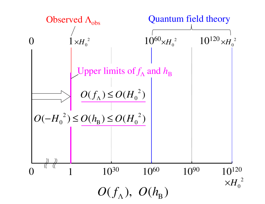
These results indicate that the second law of thermodynamics should constrain and . From Eqs. (57) and (60), the orders of the upper limits of and are likely consistent with the order of the cosmological constant measured by observations, namely . We note that is given by Eq. (9), which is based on the Planck 2018 results Planck2018 . Also, from Eq. (60), the absolute value of the order of the lower limit of is the same as the order of the upper limit.
Figure 1 shows the orders of the upper limits of the two terms, the order of Planck2018 , and the order of the theoretical value from quantum field theory Weinberg1989 ; Pad2003 ; Barrow2011 ; Bao2017 . A region for the lower limit of is not shown in this figure because the lower limit is negative and the order is the same as the order of the upper limit. We can confirm that the orders of the upper limits of the two terms are consistent with the order of . The discrepancy of orders of magnitude appears to be avoided, as if a consistent scenario could be obtained from thermodynamics.
Finally, we use the present model to discuss an important model similar to the CDM models ( and ). To this end, a deviation from the Bekenstein–Hawking entropy is considered to be close to zero but not zero. Accordingly, Eqs. (41) and (42) should reduce to and , respectively. Here, two parameters, and , should be close to zero because is close to zero. Therefore, the constraint on given by Eq. (46) should be satisfied, and the order of can be given by
| (61) |
In addition, the constraint on given by Eq. (57) can be written as
| (62) |
Equation (62) implies that the order of is consistent with the order of . In this sense, we can use the present model to discuss the cosmological constant problem from a thermodynamic viewpoint when is close to zero but not zero. The small deviation from the Bekenstein–Hawking entropy may play an important role in the accelerated expansion of our late Universe.
An arbitrary entropy on the horizon is considered here and, therefore, we can use various forms of entropy on the horizon; see, for example, Appendix B and Refs. Odintsov2024 ; Nojiri2024B . Before fine-tuning, we should be able to discuss thermodynamic constraints on driving terms calculated from those entropies. We expect that effective entropies, which deviate slightly from the Bekenstein–Hawking entropy, are favored in our Universe. Further studies are needed, and those tasks are left for future research.
It should be noted that, in this section, we consider and discuss the thermodynamic constraints. When (i.e., ), the two terms reduce to and , respectively, as for CDM models. In this case, Eq. (45) reduces to . In fact, Eq. (45) is used in the calculation of the constraint on , through Eq. (53). Accordingly, when , it is difficult to discuss the thermodynamic constraints. To avoid this difficulty, we consider . Various nonextensive entropies satisfy , except when . Note that we also consider , , , and .
In this paper, we examine the thermodynamic constraints on the two driving terms in a generalized cosmological model derived from the first law of thermodynamics, using an arbitrary entropy on the horizon. The thermodynamic constraints imply that the orders of the two terms are consistent with the order of the cosmological constant measured by observations. Of course, we cannot exclude all the other contributions, such as quantum field theory, because these contributions have not been examined in this study. In addition, the assumptions used here have not yet been established but are considered to be viable. The present study should contribute to a better understanding of thermodynamic scenarios, which may provide new insights into the discussion of the cosmological constant problem.
VI Conclusions
The first and second laws of thermodynamics should lead to a consistent scenario for discussing the cosmological constant problem. To establish such a thermodynamic scenario, we have derived cosmological equations in a flat FLRW universe from the first law, using an arbitrary entropy on the horizon. The derived cosmological equations implicitly include extra driving terms. Therefore, we have systematically reformulated the cosmological equations using a general formulation that includes two extra driving terms, and , explicitly. The present model is essentially equivalent to that derived in Ref. Odintsov2024 , but is suitable for the discussion of thermodynamic constraints.
Based on the second law of thermodynamics, we have universally examined the thermodynamic constraints on the two terms in the present model. It is found that a variation in the deviation of from the Bekenstein–Hawking entropy plays an important role in the thermodynamic constraints. In our late Universe, the second law should constrain both the upper limit of and the upper and lower limits of . The upper limits imply that the orders of the two terms are consistent with the order of the cosmological constant measured by observations. The lower limit of leads to a constraint on , and the absolute value of the order of the lower limit is likely consistent with the order of as well. In particular, when the deviation is close to zero but not zero, and should reduce to zero and a constant (consistent with the order of ), respectively, as if a consistent and viable scenario could be obtained from thermodynamics. The thermodynamic scenario may imply that the accelerated expansion of our Universe is related to the small deviation from the Bekenstein–Hawking entropy.
Appendix A Derivation of cosmological equations
In this appendix, we derive cosmological equations from the first law of thermodynamics based on the work of Odintsov et al. Odintsov2024 . The cosmological equations are considered to constitute a generalized cosmological model derived from the first law. Substituting given by Eq. (25) into Eq. (24) yields
| (63) |
Solving Eq. (63) with regard to , substituting given by Eq. (20) and into the resultant equation, and performing several operations yields Odintsov2024
| (64) |
where given by Eq. (16) is used for . Conversely, using the form of the Bekenstein–Hawking entropy allows us to write as
| (65) |
where given by Eq. (14) and given by Eq. (13) are applied. Based on Ref. Odintsov2024 , we use a symbol with brackets, namely . To this end, in the above calculation, and are applied and, therefore, corresponds to .
Substituting Eq. (64) into Eq. (65) yields
| (66) |
Calculating this equation gives Odintsov2024
| (67) |
The above equation corresponds to Eq. (5). Substituting given by Eq. (25) into Eq. (67) yields
| (68) |
We can rearrange Eq. (68) as
| (69) |
or equivalently,
| (70) |
Integrating Eq. (70) and applying yields
| (71) |
where is an integral constant and should be given by . Equation (71) is the Friedmann equation derived from the first law of thermodynamics, which is examined in Ref. Odintsov2024 . In Sec. IV, we reformulate those cosmological equations, based on the general formulation introduced in Sec. II.
Appendix B Present model for a power-law-corrected entropy
In this appendix, as a specific entropy, we apply a power-law-corrected entropy to the present model. The power-law-corrected entropy suggested by Das et al. Das2008 is based on the entanglement of quantum fields between the inside and outside of the horizon and has been applied to holographic equipartition models Koma11 ; Koma12 ; Koma14 . As far as we know, the power-law-corrected entropy has not yet been applied to the present model. Note that several forms of entropy have been examined in, for example, the recent review by Nojiri et al. Nojiri2024B and the references therein.
The power-law-corrected entropy Radicella2010 can be written as
| (72) |
where is a dimensionless parameter given by
| (73) |
and and are considered to be dimensionless constant parameters. The crossover scale is likely identified with Radicella2010 . When , reduces to . In this study, is assumed to be positive for an accelerating universe Koma11 and, therefore, is obtained from Eq. (73). We note that and may be independent free parameters Koma14 .
We now apply to the present model and calculate two extra driving terms, and . For this, we first calculate . Using Eq. (30), replacing by , and applying Eq. (74) yields
| (75) |
Here has been replaced by , using a dimensionless positive constant , to obtain a simple formulation equivalent to a power-law term examined in previous work Koma11 ; Koma12 ; Koma14 .
Integrating Eq. (75) with regard to and applying yields
| (76) |
where is an integral constant. Substituting Eq. (76) into Eq. (41) yields
| (77) |
where is and is considered to be non-negative. The second term on the right side is a power-law term proportional to . Similarly, using , we calculate . Substituting Eq. (75) into Eq. (42) yields
| (78) |
The term includes . Equations (77) and (78) imply that is non-negative, whereas is non-positive when and are considered from observations Hubble2017 , where and are also used.
Finally, we discuss the ratio of the two terms. Dividing Eq. (78) by Eq. (77) and setting for simplicity yields
| (79) |
The solution to Eq. (79) is negative when . In this case, applying to Eq. (79) gives
| (80) |
Here is assumed for a non-negative horizon temperature, as examined in Sec. III. Equation (80) indicates that is larger than when . In particular, the term tends to be dominant when a small positive is considered.
In this way, we can study the two terms in the present model for a power-law-corrected entropy. Of course, the thermodynamic constraints on the two terms can be examined by applying results in Sec. V. In addition, we can discuss the background evolutions of the universe in this specific model from a thermodynamic viewpoint. These tasks are left for future research.
References
- (1) S. Perlmutter et al., Nature (London) 391, 51 (1998); A. G. Riess et al., Astron. J. 116, 1009 (1998).
- (2) O. Farooq, F. R. Madiyar, S. Crandall, B. Ratra, Astrophys. J. 835, 26 (2017).
- (3) N. Aghanim et al., Astron. Astrophys. 641, A6 (2020).
- (4) S. Weinberg, Rev. Mod. Phys. 61, 1 (1989); V. Sahni, A. A. Starobinsky, Int. J. Mod. Phys. D 9, 373 (2000); S. M. Carroll, Living Rev. Relativity 4, 1 (2001).
- (5) T. Padmanabhan, Phys. Rep. 380, 235 (2003); R. Bousso, Gen. Relativ. Gravit. 40, 607 (2008).
- (6) J. D. Barrow, D. J. Shaw, Phys. Rev. Lett. 106, 101302, (2011).
- (7) N. Bao, R. Bousso, S. Jordan, B. Lackey, Phys. Rev. D 96, 103512 (2017); N. G. Sanchez, Phys. Rev. D 104, 123517 (2021).
- (8) K. Freese, F. C. Adams, J. A. Frieman, E. Mottola, Nucl. Phys. B287, 797 (1987); J. M. Overduin, F. I. Cooperstock, Phys. Rev. D 58, 043506 (1998).
- (9) S. Nojiri, S. D. Odintsov, Phys. Lett. B 639, 144 (2006); J. Solà, J. Phys. Conf. Ser. 453, 012015 (2013).
- (10) M. Rezaei, M. Malekjani, J. Solà Peracaula, Phys. Rev. D 100, 023539 (2019).
- (11) S. Basilakos, M. Plionis, J. Solà, Phys. Rev. D 80, 083511 (2009); M. Rezaei, J. Solà Peracaula, M. Malekjani, Mon. Not. R. Astron. Soc. 509, 2593 (2022).
- (12) J. D. Barrow, Phys. Lett. B 180, 335 (1986); J. A. S. Lima, R. Portugal, I. Waga, Phys. Rev. D 37, 2755 (1988).
- (13) I. Brevik, S. D. Odintsov, Phys. Rev. D 65, 067302 (2002); S. D. Odintsov, D. Sáez-Chillón Gómez, G. S. Sharov, Phys. Rev. D 101, 044010 (2020).
- (14) J. Yang, Rui-Hui Lin, Xiang-Hua Zhai, Eur. Phys. J. C 82, 1039 (2022).
- (15) I. Prigogine, J. Geheniau, E. Gunzig, P. Nardone, Proc. Natl. Acad. Sci. U.S.A. 85, 7428 (1988).
- (16) M. O. Calvão, J. A. S. Lima, I. Waga, Phys. Lett. A 162, 223 (1992); J. A. S. Lima, A. S. M. Germano, L. R. W. Abramo, Phys. Rev. D 53, 4287 (1996).
- (17) M. P. Freaza, R. S. de Souza, I. Waga, Phys. Rev. D 66, 103502 (2002); V. H. Cárdenas, M. Cruz, S. Lepe, S. Nojiri, S. D. Odintsov, Rev. D 101, 083530 (2020).
- (18) T. Harko, Phys. Rev. D 90, 044067 (2014); S. R. G. Trevisani, J. A. S. Lima, Eur. Phys. J. C 83, 244 (2023).
- (19) G. ’t Hooft, Conf. Proc. C 930308, 284 (1993) [arXiv:gr-qc/9310026]; L. Susskind, J. Math. Phys. 36, 6377 (1995); R. Bousso, Rev. Mod. Phys. 74, 825 (2002).
- (20) D. A. Easson, P. H. Frampton, G. F. Smoot, Phys. Lett. B 696, 273 (2011); Y. F. Cai, E. N. Saridakis, Phys. Lett. B 697, 280 (2011).
- (21) S. Basilakos, J. Solà, Phys. Rev. D 90, 023008 (2014).
- (22) N. Komatsu, S. Kimura, Phys. Rev. D 87, 043531 (2013), Phys. Rev. D 88, 083534 (2013).
- (23) N. Komatsu, S. Kimura, Phys. Rev. D 90, 123516 (2014); Phys. Rev. D 92, 043507 (2015).
- (24) N. Komatsu, S. Kimura, Phys. Rev. D 89, 123501 (2014).
- (25) N. Komatsu, S. Kimura, Phys. Rev. D 93, 043530 (2016).
- (26) E. M. C. Abreu, J. A. Neto, Phys. Lett. B 824, 136803 (2022).
- (27) H. Gohar, V. Salzano, Phys. Rev. D 109, 084075 (2024).
- (28) T. Padmanabhan, Classical Quantum Gravity 21, 4485 (2004).
- (29) Fu-Wen Shu, Y. Gong, Int. J. Mod. Phys. D 20, 553 (2011).
- (30) T. Padmanabhan, arXiv:1206.4916 [hep-th]; Res. Astron. Astrophys. 12, 891 (2012).
- (31) R. G. Cai, J. High Energy Phys. 1211 (2012) 016; S. Chakraborty, T. Padmanabhan, Phys. Rev. D 92, 104011 (2015).
- (32) M. Hashemi, S. Jalalzadeh, S. V. Farahani, Gen. Relativ. Gravit. 47, 53 (2015).
- (33) H. Moradpour, Int. J. Theor. Phys. 55, 4176 (2016).
- (34) N. Komatsu, Eur. Phys. J. C 77, 229 (2017).
- (35) N. Komatsu, Phys. Rev. D 96, 103507 (2017).
- (36) N. Komatsu, Phys. Rev. D 99, 043523 (2019).
- (37) N. Komatsu, Eur. Phys. J. C 83, 690 (2023).
- (38) T. Padmanabhan, Comptes Rendus Physique 18, 275 (2017).
- (39) Fei-Quan Tu, Yi-Xin Chen, Bin Sun, You-Chang Yang, Phys. Lett. B 784, 411 (2018).
- (40) Fei-Quan Tu, Yi-Xin Chen, Qi-Hong Huang, Entropy 21, 167 (2019).
- (41) S. Nojiri, S. D. Odintsov, T. Paul, Symmetry 13, 928 (2021).
- (42) P. B. Krishna, T. K. Mathew, Phys. Rev. D 96, 063513 (2017); Phys. Rev. D 99, 023535 (2019).
- (43) P. B. Krishna, V. T. H. Basari, T. K. Mathew, Gen. Relativ. Gravitat. 54, 58 (2022).
- (44) G. R. Chen, Eur. Phys. J. C 82, 532 (2022).
- (45) G. G. Luciano, Phys. Lett. B 838, 137721 (2023).
- (46) M. Muhsinath, V. T. H. Basari, T. K. Mathew, Gen. Relativ. Gravitat. 55, 43 (2023).
- (47) M. T. Manoharan, N. Shaji, T. K. Mathew, Eur. Phys. J. C 83, 19 (2023).
- (48) N. Komatsu, Phys. Rev. D 100, 123545 (2019).
- (49) N. Komatsu, Phys. Rev. D 102, 063512 (2020).
- (50) N. Komatsu, Phys. Rev. D 103, 023534 (2021).
- (51) N. Komatsu, Phys. Rev. D 105, 043534 (2022).
- (52) N. Komatsu, Phys. Rev. D 108, 083515 (2023).
- (53) N. Komatsu, Phys. Rev. D 109, 023505 (2024).
- (54) N. Komatsu, Eur. Phys. J. C 85, 35 (2025).
- (55) R. G. Cai, S. P. Kim, J. High Energy Phys. 02 (2005) 050.
- (56) R. G. Cai, L. M. Cao, N. Ohta, Phys. Rev. D 81, 061501(R) (2010).
- (57) R. G. Cai, L. M. Cao, Phys. Rev. D 75, 064008 (2007).
- (58) R. G. Cai, L. M. Cao, Y. P. Hu, Classical Quantum Gravity 26, 155018 (2009); S. Mitra, S. Saha, S. Chakraborty, Phys. Lett. B 734, 173 (2014).
- (59) A. Sheykhi, Phys. Rev. D 81, 104011 (2010); S. Mitra, S. Saha, S. Chakraborty, Mod. Phys. Lett. A 30, 1550058 (2015).
- (60) K. Karami, A. Abdolmaleki, Z. Safari, S. Ghaffari, J. High Energy Phys. 08 (2011) 150. A. Sheykhi, S. H. Hendi, Phys. Rev. D 84, 044023 (2011).
- (61) F. L. Dezaki, B. Mirza, Gen. Relativ. Gravit. 47, 67 (2015).
- (62) C. A. S. Silva, Eur. Phys. J. C 78, 409 (2018); C. Silva, Nucl. Phys. B 998, 116402 (2024).
- (63) P. S. Ens, A. F. Santos, Phys. Lett. B 835,137562 (2022).
- (64) A. Sheykhi, Phys. Rev. D 103, 123503 (2021); A. Sheykhi, Phys. Lett. B 850, 138495 (2024).
- (65) S. Nojiri, S. D. Odintsov, T. Paul, Phys. Lett. B 835, 137553 (2022).
- (66) M. Akbar, R. G. Cai, Phys. Rev. D 75 084003 (2007).
- (67) M. Akbar, R. G. Cai, Phys. Lett. B 648, 243 (2007).
- (68) R. G. Cai, L. M. Cao, Y. P. Hu, J. High Energy Phys. 08 (2008) 090.
- (69) L. M. Sánchez, H. Quevedo, Phys. Lett. B 839, 137778 (2023).
- (70) S. Nojiri, S. D. Odintsov, T. Paul, S. SenGupta, Phys. Rev. D 109, 043532 (2024).
- (71) S. D. Odintsov, S. D’Onofrio, T. Paul, Physics of the Dark Universe 42 (2023) 101277.
- (72) S. D. Odintsov, T. Paul, S. SenGupta, Phys. Rev. D 109, 103515 (2024).
- (73) S. D. Odintsov, S. D’Onofrio, T. Paul, Phys. Rev. D 110, 043539 (2024).
- (74) S. Nojiri, S. D. Odintsov, T. Paul, Universe 2024, 10, 352.
- (75) A. Khodam-Mohammadi, M. Monshizadeh, Phys. Lett. B 843,138066 (2023); A. Khodam-Mohammadi, Mod. Phys. Lett. A 39, 2450146 (2024).
- (76) S. W. Hawking, Phys. Rev. Lett. 26, 1344 (1971); Nature (London) 248, 30 (1974); Commun. Math. Phys. 43, 199 (1975); Phys. Rev. D 13, 191 (1976); J. D. Bekenstein, Phys. Rev. D 7, 2333 (1973); Phys. Rev. D 9, 3292 (1974); Phys. Rev. D 12, 3077 (1975).
- (77) S. Das, S. Shankaranarayanan, S. Sur, Phys. Rev. D 77, 064013 (2008).
- (78) N. Radicella, D. Pavón, Phys. Lett. B 691, 121 (2010).
- (79) C. Tsallis, L. J. L. Cirto, Eur. Phys. J. C 73, 2487 (2013).
- (80) T. S. Biró, V. G. Czinner, Phys. Lett. B 726, 861 (2013).
- (81) J. D. Barrow, Phys. Lett. B 808, 135643 (2020).
- (82) S. Nojiri, S. D. Odintsov, V. Faraoni, Phys. Rev. D 105, 044042 (2022).
- (83) B. Ryden, Introduction to Cosmology (Addison-Wesley, Reading, MA, 2002).
- (84) T. Jacobson, Phys. Rev. Lett. 75, 1260 (1995).
- (85) T. Padmanabhan, Mod. Phys. Lett. A 25, 1129 (2010).
- (86) E. Verlinde, J. High Energy Phys. 04 (2011) 029.
- (87) G. W. Gibbons, S. W. Hawking, Phys. Rev. D 15, 2738 (1977).
- (88) S. A. Hayward, Classical Quantum Gravity 15, 3147, (1998).
- (89) S. A. Hayward, R. D. Criscienzo, M. Nadalini, L. Vanzo, S. Zerbini, Classical Quantum Gravity 26, 062001 (2009).
- (90) C. A. Egan, C. H. Lineweaver, Astrophys. J. 710, 1825 (2010).