Could the “Wow” signal have originated from a stochastic repeating beacon?
Abstract
The famous “Wow” signal detected in 1977 remains arguably the most compelling SETI signal ever found. The original Big Ear data requires that the signal turned on/off over the span of minutes (time difference between the dual antennae), yet persisted for 72 seconds (duration of a single beam sweep). Combined with the substantial and negative follow-up efforts, these observations limit the allowed range of signal repeat schedules, to the extent that one might question the credibility of the signal itself. Previous work has largely excluded the hypothesis of a strictly periodic repeating source, for periods shorter than 40 hours. However, a non-periodic, stochastic repeater remains largely unexplored. Here, we employ a likelihood emulator using the Big Ear observing logs to infer the probable signal properties under this hypothesis. We find that the maximum a-posteriori solution has a likelihood of 32.3%, highly compatible with the Big Ear data, with a broad 2 credible interval of signal duration secs mins and mean repeat rate days days-1. We extend our analysis to include 192 hours of subsequent observations from META, Hobart and ATA, which drops the peak likelihood to 1.78%, and thus in tension with the available data at the 2.4 level. Accordingly, the Wow signal cannot be excluded as a stochastic repeater with available data, and we estimate that 62 days of accumulated additional observations would be necessary to surpass 3 confidence.
keywords:
extraterrestrial intelligence — methods: statistical1 Introduction
In 1977, the Ohio State University Radio Observatory recorded a strong (30 ), narrowband ( kHz) signal near the 21 cm hydrogen line (Kraus, 1979). The signal, discovered during a search for extraterrestrial intelligence (SETI), bore a remarkable resemble to the properties expected from an alien transmitter, leading the volunteer analyst Jerry Ehman to famously annotate “Wow!” on the computer printout (Ehman, 1998). The time-dependent intensity of the emission matched the antenna pattern signature of a transiting celestial source (Gray & Marvel, 2001), unlike what would be expected for interference. This behaviour, combined with its narrowband nature and location near 21 cm, leads to a trifecta of features long predicted from a genuine SETI signal (Cocconi & Morrison, 1959), causing Wow to be one of the few astronomical observations that have bled into popular culture.
Although the field was observed many times, Wow was only seen once during the entire baseline of observations from the Ohio State University Radio Observatory, known as the “Big Ear” (Kraus, 1979). Further, Wow only occurred in one beam of a dual-beam transit antenna system (Dixon & Cole, 1977), implying that the signal switched on/off in the brief interval between the two beams sweeping over the source ( minutes). However, Wow appears consistent with being continuously “on” during the 72 seconds of one beam passing over the source.
Despite numerous attempts to replicate the detection of Wow (Gray, 1994; Gray & Marvel, 2001; Gray & Ellingsen, 2002; Harp et al., 2020), the signal has not been observed again. The single-beam detection and lack of any repetition (especially with greater sensitivity, longer observations and broader spectral coverage), ostensibly places considerable pressure on the credibility of the Wow signal111For example, in an interview with the http://www.bigear.org/wow.htm in 1994, Jerry Ehman remarked “We should have seen it again when we looked for it 50 times. Something suggests it was an Earth-sourced signal that simply got reflected off a piece of space debris.”. However, a recent Bayesian formulation of one-off events showed that at least an order-of-magnitude more data than that used in the original discovery is often required to place statistically significant tension on a signal’s credibility (Kipping, 2021).
Motivated by that work, we here explore a rigorous statistical approach to address: i) how likely is it that Wow repeats but has simply been missed by follow-up efforts to date, and ii) if so, what are the most likely properties of the signal under this scenario?
There are two basic ways that Wow could remain a genuine SETI signal yet remain consistent with all observations to date. It could either be a non-continuous emission source and/or a continuous source that drifts in frequency. Regarding the latter possibility, Wow was detected in channel 2 of 50 by Big Ear (Kraus, 1979), each with a 10 kHz band. Given that the signal appears/disappears over a 3 minute interval, a drift rate of 20 kHz/3 minutes Hz s (i.e. nHz) could conceivably explain this222Such a signal would drift 7.2 kHz during the 72 second duration of a single-beam, and thus would also plausibly be confined to a single 10 kHz channel.. We note that this would be considered at the upper fringes of plausibility for a genuine SETI signal (Sheikh et al., 2019); for example the Earth’s fractional drift rate from orbital and rotational motion is three orders-of-magnitude smaller. Further, subsequent observations by Gray & Ellingsen (2002) used a band five times wider than than of Big Ear (500 kHz) spanning six 14-hour continuous blocks, yet reported no Wow-like repetition.
A non-continuous signal is more interesting and might be expected from an economics perspective, as suggested by Benford, Benford, & Benford (2008). A strictly periodic repeater might be expected if the source behaved akin to a lighthouse, perhaps as a continuous source rotating across the sky or programmed to emit only periodically in our direction. Gray & Ellingsen (2002) and Harp et al. (2020) excluded strictly periodic repeaters with periods below 40 hours and longer timescales become increasingly improbable to fortuitously allow the Wow signal being detected in the first place. To date, there has been no investigation of a non-periodic, stochastic repeater though. A stochastic repeater could be attractive from the perspective of avoiding sampling holes. For example, signals that repeat once per 24 hours both risk evading our observing cadence as well being immediately suspicious as spurious even if recorded. An intermittent signal could also manifest due to scintillation within the interstellar medium, in particular for sources parsecs away (Cordes, Lazio, & Sagan, 1997). The underlying cause of the intermittency is not of principal interest here, rather we consider that such intermittency is feasible and the compatibility of existing observations with such a scenario has not been extensively studied for Wow.
In this work, we investigate this possibility by evaluating the plausibility of said hypothesis and the corresponding required signal properties. Although Kipping (2021) presents a framework for such an analysis, that work is only valid when the data are homogenous, regular and no substantial changes to the observing instruments nor strategy are implemented. In order to account for the sparse, irregular sampling of Big Ear, as well as the subsequent observations, we require a more detailed approach that emulates the detection efficiency of the instrument for various proposed signal forms. To this end, Section 2 presents such an emulator, which is then used in Section 3 to infer a posterior distribution for the signal form. We extend this analysis in Section 4 to include observations besides from that of Big Ear, and conclude in Section 5.
2 The likelihood of a Wow-like signal
2.1 Model for the Signal(s)
Searches for strict periodicity can be readily achieved using classic periodogram techniques. Stochastic repeaters, in contrast, may evade detection using such techniques. Accordingly, we here seek to test the specific hypothesis of a stochastic repeater.
In what follows, we assume that the source maintains a uniform rate of signal production over any fixed interval of time within the baseline of the Big Ear observations. This essentially corresponds to a kind of Copernican Principle in time - we assume that the Big Ear observations do not occupy a special point in time when the signal source changed its emission mode (for example). Indeed, this assumption demands that the mean number of signals produced per unit time (in our direction) is the same when Big Ear began observing the source, as when it finished. This defines a Poisson process, for which the interval between individual signals will follow an exponential distribution. Accordingly, the signal will occur at a time
| (1) |
where is an exponential distribution of mean . For a given choice of , we thus begin our simulation by iteratively populating a list of signal mid-times using Equation 1, where we start with but ultimately discard this initial entry.
The signal is also characterised by a duration. In what follows, we assume that the signal is a top-hat persisting for a time (with no variability), since this is both consistent with the Wow signal and represents the simplest possible model. If , the two signals are effectively merged into a longer continuous one.
2.2 Model for the Observations
The observations are modelled using the observing logs of the Wow field from Big Ear itself. In September 1985, co-author Robert Gray visited OSU where the logs were reviewed and noted. Print outs were pulled from the OSU archives by Marc Abel, who located runs from 122 days spanning August 1977 to March 1984. Data near the Wow locale was examined for each day, with the locale defined as near RA 19 17 in 1977, and RA 19 22 and 19 25 subsequently, since a horn squint correction had presumably been applied by 1978.
Excluding observations more than 20’ north or south of the Wow declination, or days with bad data (e.g. clock off, printer failure, power failure), we find 90 useful visits, which are listed in Table 1.
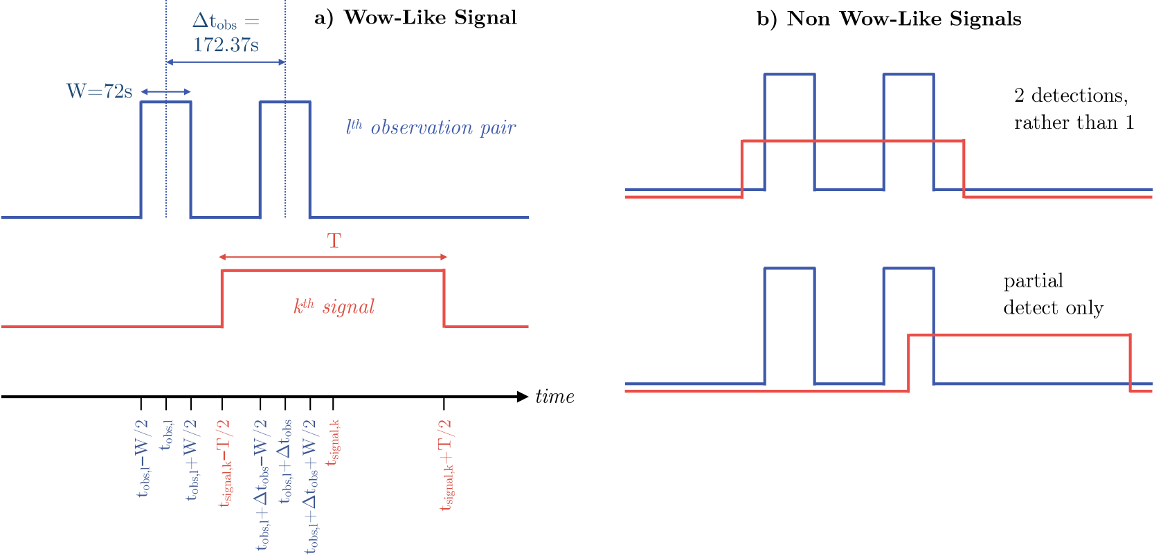
These dates are used to define a set of representative observations in our simulation, with the first observation occurring at days, and subsequent observations offset in time from this reference point according to their observation date. Each observation in fact a pair of measurements, since the Big Ear horns are physically separated and thus a sky source passes over each. Accordingly, we define the first of these two occurring at a mid-time of (for the observation) and the next occurring at , where seconds represents the temporal offset.
Each of the pair of observations is modelled as lasting for 72 seconds. For a “detection” to occur, we define that a signal must be throughout the entire duration of this 72-second window. We thus cycle through each observation ( in total) and query whether any of the generated signals lead to a detection. After cycling through all observations, we tally up the total number of detections. Illustrative examples of both Wow-like and non Wow-like signals are depicted in Figure 1.
2.3 The Likelihood of a Wow-Like Signal
The process of generating a set of injected signals, comparing them to our simulated observations and tallying up the number of detections defines a single realisation. Since the signal generation process is stochastic, a statistical interpretation requires repeating many realisations for a given choice of and . In practice, we approach this by creating a “while” loop that generates many realisations and continues until exactly one detection is made - since this is what was found for the Wow signal. The greater the number of realisations necessary, the less likely it is that the particular choice of and could reproduce Wow. Naively, one might reason that if it took realisations to get a Wow-like signal, then the probability of and producing Wow is .
For computational efficiency, we cap the maximum number of realisations in our while loop at 1000 and flag such cases appropriately. Although this single while loop provides a first estimate of probability, it is inherently uncertain given the fact only a single loop was executed. Thus, we wish to repeat the loop times, in order to improve our confidence in the estimated probability.
Since our while loop represents a binary outcome of fixed probability, then represents the number of Bernoulli trials needed to get one success, defining a geometric distribution i.e. , where represents the geometric distribution and is the probability value for this choice of and . We now wish to infer from a sequence of evaluations emerging from our while loops, which form a vector with indices of length . To accomplish this, we note that
| (2) |
where . To infer (the posterior distribution of ), we need to use Bayes theorem. Adopting a uniform prior on for simplicity, the posterior is simply the normalised likelihood given by
| (3) |
Differentiating, this has a mode (i.e. maximum a-posteriori, MAP) value of
| (4) |
which is close to our original intuition of for . However, this process also allows us to define the variance to be
| (5) |
Using these results we can say that after while loops, each of which took realisations to obtain a Wow-like signal, we infer the MAP likelihood of the choice of and to be with a precision (fractional error) of . We thus continue through the while loops until the precision falls below 10% - which we qualify as a “good” estimate of .
2.4 Likelihood Emulator
From before, represents the maximum a-posteriori probability of obtaining a Wow-like signal with the 90 days of Big Ear data, given a choice of and . In moving towards inferring and , can be considered to be the (most probable) likelihood of obtaining the data (here defined as a single detection in the 90 pairs of observations) given and . Thus, we define
| (6) |
To make progress, we need to be able to vary and and evaluate likelihoods quickly, to exploit Bayesian inference methods. Given the computational expensive nature of even a single likelihood evaluation (sometimes taking many hours), we elected to build a grid of and values across which we could pre-calculate the likelihoods and then use them to build a likelihood emulator at intermediate values. To this end, we set up a square grid of plausible values for each. The grid was chosen to be log-uniformly spaced from to and to , such that
| (7) |
where and are the integer indices running from 1 to . We set seconds, which defines the minimum allowed duration given that the signal shape appears consistent with a continuous emission. For , we chose a maximum at least two orders of magnitude larger and specifically adopted days. For and , we chose to bracket them three orders of magnitude either side of , giving days-1 and days-1.
Our later parameter explorations found that this initial grid did not support certain regions of high likelihood space and needed to be expanded. To accomplish this, we simply increased the indices and beyond 100. Specifically, we ran up to and . This means that in practice the maximum allowed value is not in fact , but rather , and similarly for , where
| (8) |
which evaluates to days and days-1.
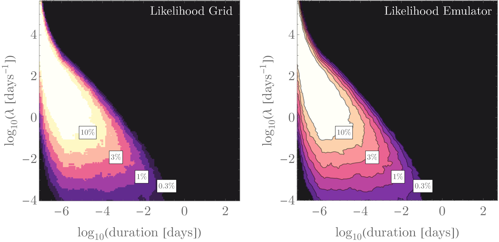
Since our grid is regular and evenly spaced (in log space), it is amenable to interpolation. To this end, we use a bi-cubic spline interpolation of the grid. As shown in Figure 2, this leads to an accurate and quick emulator across the high likelihood region of interest.
3 The a-posteriori “Wow” signal properties
3.1 MCMC
Having established a likelihood emulator supported over the range and , we now turn to inferring the joint posterior distribution of and , given the data . This can be achieved through Bayes theorem:
| (9) |
For the prior, , we assume that the priors are independent and follow log-uniform distributions over their supported range. This is most easily achieved by simply walking in and space directly, which is also convenient as this is the native sampling the grid used for the likelihood emulator. The limits on the walkers are set to that of our likelihood grid, since outside this region we cannot reliably emulate the likelihood.
We sample the joint posterior distribution using Markov Chain Monte Carlo algorithm and Metropolis walkers, calculating the posterior probability as a product of our likelihood emulator and the prior (which is uniform in this parameterisation). Each walker completes 110,000 accepted steps, burning off the first 10,000. The starting point for the chain is randomly drawn from the joint prior. We repeat for 100 walkers and combine the final results, with a thinning of a factor of 10 to leave us with posterior samples. Chains and posterior distributions were inspected to ensure convergence and good mixing.
3.2 Analysis
The joint posterior distribution is depicted in Figure 3. We find that the marginalised duration distribution peaks close to the lower boundary condition. Since MCMC samplers cannot make jumps below the prior minimum threshold, a slightly positively skewed posterior is expected even when the result is consistent with the minimum. Accordingly, we here conclude that there is no clear lower limit on the signal duration, besides from the constraint that it appears consistent with being fully-on during the window in which it was caught (i.e. seconds). However, we find that long duration signals are disfavoured, which can be understood by the fact that they are increasingly unlikely to have only been detected once during the ensemble of Big Ear observations. Indeed, from this, we can place an upper limit that minutes to confidence (95.45%).
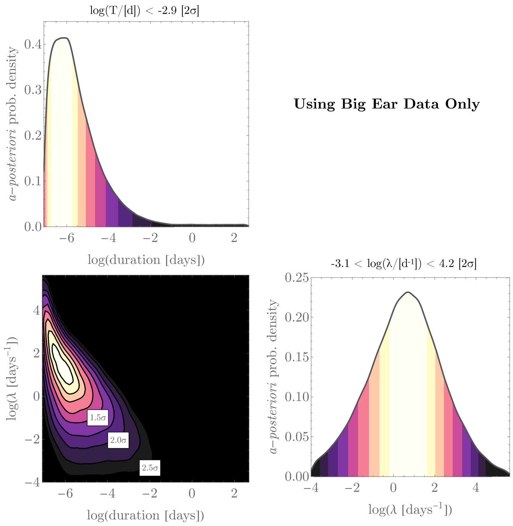
For , the mean rate of signal emission, we find a broad but peaked posterior with a maximum at days-1 (i.e. twice per day). We can see that is inversely correlated to but compresses in a narrow region at low . This “fine-tuning” reduces the marginalised posterior density in this region, and ultimately gets truncated by the lower boundary on . Very frequent repeat times are only compatible with the data at extremely short durations, in order to explain the lack of additional detections. Together, these constraints imply that is bound within the interval days-1 to days-1 to 2 .
4 Accounting for additional follow-up
4.1 Follow-up Observations
Of course, besides from the original Big Ear observations, there have been several efforts to re-observe the field and look for repetitions, without success. In Gray (1994), the field was observed using the ultranarrowband Harvard/Smithsonian-META system (Horowitz et al., 1986), tracking for up to 4 hour at a time. Gray & Marvel (2001) performed the second attempt with the Very Large Array, tracking the field for no more than 22 minutes a time. Gray & Ellingsen (2002) performed far longer observations with the University of Tasmania’s Hobart 26 m radio telescope, tracking the field for 14 hours continuously on six separate days. Finally, the Allan Telescope Array was used by Harp et al. (2020), accumulating over 100 hours on target for 30 to 180 minutes each time. In all cases, we note that the observations were sufficiently sensitive to have recovered a repeat of the Wow signal to high confidence.
4.2 Incorporating the Hobart Constraints
Amongst the four follow-up efforts highlighted above, the Gray & Ellingsen (2002) data with Hobart is most amenable to incorporating into our analysis, since the observing window is approximately the same each time (14 hours) and only six sets were taken. The dates of the observations are provided in Gray & Ellingsen (2002) and thus we could easily imagine directly extending our likelihood formalism to include these dates. However, a much simpler approach would be to ignore the dates and rather just assume that each 14-hour window is an independent and fair sample over all time within which no detection was made. For a hour block, the probability of a Poisson process not yielding a single success equals , and to evade detection in six independent draws would be . This serves as an additional likelihood term which we can append to the Big Ear likelihood emulator. With this simple change, we repeated the MCMC analysis using an otherwise identical setup.
The updated chain found that the maximum likelihood dropped from 32.3% using Big Ear alone, to 3.27%, thus placing tension on the stochastic repeater hypothesis at the 2.1 level. This peak occurs at days-1 and s. Evaluating the likelihood of this position using the Big Ear likelihood emulator alone (ignoring the Hobart data) yields 7.40%. Thus, the likelihood shifts from 7.40% to 3.27% - a factor of 0.442 of the original value, which of course simply equals . Using this point of highest likelihood, we can test the accuracy of our assumption of independence.
To this end, we used the dates of the Hobart observations and generated 1000 Poisson processes with a mean rate and duration and counted how many detections Hobart would have seen. From this, we measure 439 zero-count cases - consistent with the real observations of Gray & Ellingsen (2002). Thus, we find that a more realistic calculation that accounts for the specific timings of the observations yields a Hobart-likelihood at and of - a value fully consistent with the much simpler independence assumption. On this basis, we argue that our simplifying assumption is justified and produces an accurate final posterior.
From our revised joint posterior, we obtain credible intervals of d-1 and .
4.3 Extending to Other Observations
Our approach for incorporating the Hobart observations can be extended to other data sets too. Recall that for Hobart, the additional likelihood term was , since 6 sets of baselines were taken. This is equivalent to adding a single penalty of duration (i.e. 84 hours). Accordingly, even if the other observations did not use the same observational window each, we can still include them by simply counting up the total observing time of each (on the Wow field).
From Gray (1994), we find 8 hours on each of the two possible Wow positions. Gray & Marvel (2001) dwelled no longer than 22 minutes on the field and used a variety of observing modes, and thus we elected to not include these data as their temporal constraining power is small compared to Hobart. In contrast, the ATA 100 hour campaign from Harp et al. (2020) more than doubles the baseline and thus provides a key constraint. Together then, we add a third likelihood term equal to , where hours.
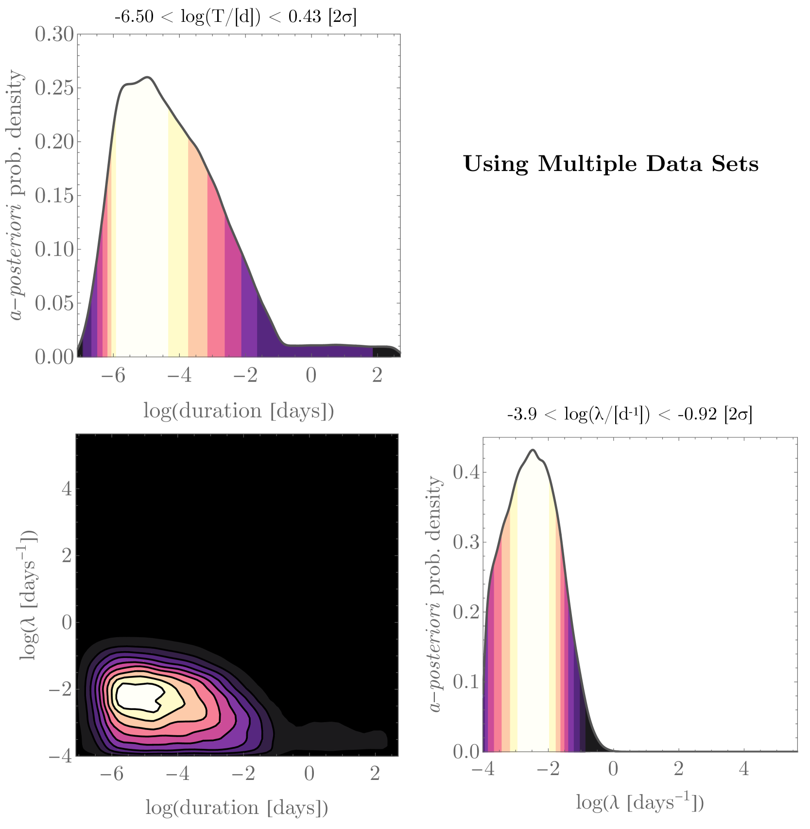
With this change, the final maximum likelihood is 1.78% (2.37 ), occurring at s and days-1. The final joint posterior is plotted in Figure 4, where we report a revised 2 credible interval of and d-1. In practice, the joint posterior is not significantly changed by the inclusion of the other observational constraints.
5 Discussion
Our work has used a likelihood emulator derived from the Big Ear observing logs to investigate the properties of the Wow signal, under the assumption it is a stochastic repeater. Here, we discuss the implications of this result, and validity of our underlying assumption.
We’ll begin with the latter. It must be acknowledged that have no evidence that the Wow signal is a repeating signal. Indeed, the lack of any repeat is what makes the signal so tantalising and ultimately motivates our study to investigate how viable the repeating hypothesis is. However, even if the signal is non-repeating, it is technically consistent with our formalism in the limiting case that the mean repeat time tends to infinity (i.e. ). With just a single pulse produced over all cosmic time, it’s incredibly improbable that the Big Ear would have coincidentally been looking at the correct place at the correct moment to catch it. Indeed, our analysis with the Big Ear data alone has a marginalised posterior density that tends to 0 in the limit of .
Using just the Big Ear data, strict periodic signals are challenging to constrain since the field was observed briefly just twice per day, meaning that periodic signals can easily fall out of phase with an initial detection. This possibility was investigated in Gray & Ellingsen (2002), although the duration of the signal was fixed to three scenarios of s, s and s, rather than freely fitted as done in this work. Gray & Ellingsen (2002) report that periods of below one day had a % likelihood of reproducing the observations, peaking at 35% for signals of approximately an hour period.
To compare to our stochastic repeater analysis, we find a peak likelihood of 32.3% for a signal of duration s and mean rate days-1 ( hours mean repeat time). Thus, the stochastic assumption can be seen to allow for even higher compatibility with the original data, although the timescales involved of the best fitting signals are not grossly different. This of course is not surprising given the inherently more “slippery” nature of a stochastic process.
Of course, follow-up observations have placed much stronger constraints on strictly periodic signals. Gray & Ellingsen (2002) completely excludes strict periodicity for periods less than 14 hours. Going further, Harp et al. (2020) provides the tightest constraints to date, finding that periods from 0 to 40 hour would have been detected in 99% of their realisations.
As shown in Section 4, including these additional observations into our analysis provides tighter constraints on the joint posterior. Most importantly, the inclusion of this data reduces the maximum likelihood from 32.3% with Big Ear alone to 1.78% (2.37 ). Thus, the data collected to date are surprising under the stated hypothesis, but not at the level typically needed to reject a hypothesis ( or more). We repeated the follow-up MCMC but adding hours of simulated null results to investigate how much data would be needed to reach a 3 threshold. Iterating, we found that 62 days of accumulated additional observations would be needed333Note that this timescale is insensitive to the priors used since it represents simply the maximum likelihood value.. On this basis, we argue that the stochastic repeater hypothesis is not yet excluded as an explanation for the Wow signal, and yet more follow-up would be necessary.
More broadly, our likelihood emulation approach provides an example of dealing with sparse, irregular observations to conduct inference of SETI signals of interest. Indeed this approach could be readily applied to other technosignature data sets, such as the Breakthrough Listen radio search (Price et al., 2020; Sheikh et al., 2021) or even non-radio searches such as in the optical (e.g. see Maire et al. 2020). It is emphasised that such an approach could also be used for targets without any signals detected, in order to derive robust upper limits on a hypothesised signal’s properties (be it periodic or not).
Acknowledgments
Co-author Robert Gray tragically passed away during this work. RG devoted himself to pursuing the Wow signal throughout his career, both in science and public discourse. His insights and contributions to this enigma are unparalleled and were pivotal to this paper. DK is grateful for his generosity, time and contributions to this study, which it is hoped live up to his high standards of inquiry and curiosity.
This work was enabled thanks to supporters of the Cool Worlds Lab, including Mark Sloan, Douglas Daughaday, Andrew Jones, Elena West, Tristan Zajonc, Chuck Wolfred, Lasse Skov, Graeme Benson, Alex de Vaal Mark Elliott, Methven Forbes, Stephen Lee, Zachary Danielson, Chad Souter, Marcus Gillette, Tina Jeffcoat, Jason Rockett, Scott Hannum, Tom Donkin, Andrew Schoen, Jacob Black, Reza Ramezankhani, Steven Marks, Philip Masterson, Gary Canterbury, Nicholas Gebben, Joseph Alexander, Mike Hedlund, Dhruv Bansal, Jonathan Sturm, Rand Corporation, Ian Attard & Leigh Deacon.
Data Availability
The code used and results generated by this work are made publcily available at this URL.
References
- Benford, Benford, & Benford (2008) Benford J., Benford G., Benford D., 2008, arXiv, arXiv:0810.3964
- Cocconi & Morrison (1959) Cocconi G., Morrison P., 1959, Natur, 184, 844. doi:10.1038/184844a0
- Cordes, Lazio, & Sagan (1997) Cordes J. M., Lazio J. W., Sagan C., 1997, ApJ, 487, 782. doi:10.1086/304620
- Dixon & Cole (1977) Dixon R. S., Cole D. M., 1977, Icar, 30, 267. doi:10.1016/0019-1035(77)90158-0
- Ehman (1998) Ehman, J. R., 1998, “The Big Ear Wow! Signal: What We Know and Don’t Know About It after 20 Years”, OSURO working paper
- Gray (1994) Gray R. H., 1994, Icar, 112, 485. doi:10.1006/icar.1994.1199
- Gray & Marvel (2001) Gray R. H., Marvel K. B., 2001, ApJ, 546, 1171. doi:10.1086/318272
- Gray & Ellingsen (2002) Gray R. H., Ellingsen S., 2002, ApJ, 578, 967. doi:10.1086/342646
- Harp et al. (2020) Harp G. R., Gray R. H., Richards J., Shostak G. S., Tarter J. C., 2020, AJ, 160, 162. doi:10.3847/1538-3881/aba58f
- Horowitz et al. (1986) Horowitz P., Matthews B. S., Forster J., Linscott I., Teague C. C., Chen K., Backus P., 1986, Icar, 67, 525. doi:10.1016/0019-1035(86)90129-6
- Kipping (2021) Kipping D., 2021, MNRAS, 504, 4054. doi:10.1093/mnras/stab1129
- Kraus (1979) Kraus J., 1979, CosSe, 1, 31
- Maire et al. (2020) Maire J., Wright S. A., Werthimer D., Antonio F. P., Brown A., Horowitz P., Lee R., et al., 2020, SPIE, 11454, 114543C. doi:10.1117/12.2562786
- Price et al. (2020) Price D. C., Enriquez J. E., Brzycki B., Croft S., Czech D., DeBoer D., DeMarines J., et al., 2020, AJ, 159, 86. doi:10.3847/1538-3881/ab65f1
- Sheikh et al. (2019) Sheikh S. Z., Wright J. T., Siemion A., Enriquez J. E., 2019, ApJ, 884, 14. doi:10.3847/1538-4357/ab3fa8
- Sheikh et al. (2021) Sheikh S. Z., Smith S., Price D. C., DeBoer D., Lacki B. C., Czech D. J., Croft S., et al., 2021, NatAs, 5, 1153. doi:10.1038/s41550-021-01508-8
| Date | Days Passed | Date | Days Passed |
|---|---|---|---|
| 13-Aug-1977 | 0 | 22-Jan-1983 | 1988 |
| 14-Aug-1977 | 1 | 22-Jan-1983 | 1988 |
| 15-Aug-1977 | 2 | 23-Jan-1983 | 1989 |
| 17-Aug-1977 | 4 | 24-Jan-1983 | 1990 |
| 16-Sep-1977 | 34 | 25-Jan-1983 | 1991 |
| 17-Sep-1977 | 35 | 28-Jan-1983 | 1994 |
| 18-Sep-1977 | 36 | 29-Jan-1983 | 1995 |
| 19-Sep-1977 | 37 | 2-Feb-1983 | 1999 |
| 20-Sep-1977 | 38 | 2-Feb-1983 | 1999 |
| 21-Sep-1977 | 39 | 4-Feb-1983 | 2001 |
| 22-Sep-1977 | 40 | 5-Feb-1983 | 2002 |
| 23-Sep-1977 | 41 | 6-Feb-1983 | 2003 |
| 24-Sep-1977 | 42 | 7-Feb-1983 | 2004 |
| 25-Sep-1977 | 43 | 12-Feb-1983 | 2009 |
| 26-Sep-1977 | 44 | 14-Feb-1983 | 2011 |
| 27-Sep-1977 | 45 | 15-Feb-1983 | 2012 |
| 28-Sep-1977 | 46 | 16-Feb-1983 | 2013 |
| 29-Sep-1977 | 47 | 17-Feb-1983 | 2014 |
| 30-Sep-1977 | 48 | 18-Feb-1983 | 2015 |
| 4-Oct-1977 | 52 | 19-Feb-1983 | 2016 |
| 30-Oct-1977 | 78 | 20-Feb-1983 | 2017 |
| 10-Apr-1978 | 240 | 21-Feb-1983 | 2018 |
| 11-Apr-1978 | 241 | 22-Feb-1983 | 2019 |
| 17-Apr-1978 | 247 | 23-Feb-1983 | 2020 |
| 24-Apr-1978 | 254 | 24-Feb-1983 | 2021 |
| 25-Apr-1978 | 255 | 25-Feb-1983 | 2022 |
| 26-Apr-1978 | 256 | 26-Feb-1983 | 2023 |
| 27-Apr-1978 | 257 | 27-Feb-1983 | 2024 |
| 28-Apr-1978 | 258 | 28-Feb-1983 | 2025 |
| 1-May-1978 | 261 | 1-Mar-1983 | 2026 |
| 2-May-1978 | 261 | 7-Mar-1983 | 2032 |
| 28-Aug-1978 | 380 | 8-Mar-1983 | 2033 |
| 29-Aug-1978 | 381 | 9-Mar-1983 | 2034 |
| 30-Aug-1978 | 382 | 12-Mar-1983 | 2037 |
| 31-Aug-1978 | 383 | 13-Mar-1983 | 2038 |
| 1-Sep-1978 | 384 | 14-Mar-1983 | 2039 |
| 2-Sep-1978 | 385 | 20-Mar-1983 | 2045 |
| 3-Sep-1978 | 386 | 21-Mar-1983 | 2046 |
| 4-Sep-1978 | 387 | 23-Mar-1983 | 2048 |
| 2-Jan-1983 | 1968 | 26-Mar-1983 | 2051 |
| 3-Jan-1983 | 1969 | 28-Mar-1983 | 2053 |
| 4-Jan-1983 | 1970 | 29-Mar-1983 | 2054 |
| 7-Jan-1983 | 1973 | 26-Apr-1983 | 2082 |
| 13-Jan-1983 | 1979 | 9-May-1983 | 2095 |
| 15-Jan-1983 | 1981 | 6-Dec-1984 | 2672 |