Countable families of solutions of a limit stationary semilinear fourth-order Cahn–Hilliard equation I. Mountain pass and Lusternik–Schnirel’man patterns in
Abstract.
Solutions of the stationary semilinear Cahn–Hilliard equation
which are exponentially decaying at infinity, are studied. Using the Mounting Pass Lemma allows us the determination of two different solutions. On the other hand, the application of Lusternik–Schnirel’man (L–S) Category Theory shows the existence of, at least, a countable family of solutions.
However, through numerical methods it is shown that the whole set of solutions, even in 1D, is much wider. This suggests that, actually, there exists, at least, a countable set of countable families of solutions, in which only the first one can be obtained by the L–S min-max approach.
Key words and phrases:
stationary Cahn–Hilliard equation, variational setting, non-unique oscillatory solutions, countable family of critical points1991 Mathematics Subject Classification:
35G20, 35K521. Introduction and motivation for main problems
1.1. Models and preliminaries
This paper studies some multiplicity properties of the steady-states of the following fourth-order parabolic equation of the Cahn–Hilliard (C–H) type:
| (1.1) |
The problem is completed with bounded smooth initial data,
| (1.2) |
Assuming that data are sufficiently fast exponentially decaying at infinity, the same behaviour holds for the unique classic solution of (1.1), at least locally in time, since, for , may blow-up in finite time; see key references and results in [6] and [14].
The classic Cahn–Hilliard equation describes the dynamics of pattern formation in phase transition in alloys, glasses, and polymer solutions. When a binary solution is cooled sufficiently, phase separation may occur and then proceed in two ways: either nucleation, in which nuclei of the second phase appear randomly and grow, or, in the so-called spinodal decomposition, the whole solution appears to nucleate at once and then periodic or semi-periodic structures appear. Pattern formation resulting from phase transition has been observed in alloys, glasses, and polymer solutions. Parallelly, these types of equations possesses a great interest in biology and, after certain transformations (see below) as prototype for nerve conduction in the form of a FitzHugh–Nagumo system (cf. [17, 25]).
Cahn–Hilliard equations-type such as (1.1) have been studied by many authors during the last decades. Among some of the works where several aspects related to these equations are [2, 33, 34, 35, 36]. Additionally, one can check the surveys in [14, 20], where necessary aspects of global existence and blow-up of solutions for (1.1) are discussed in sufficient detail.
From the mathematical point of view, the non-stationary equation (1.1) involves a fourth order elliptic operator and it contains a negative viscosity term. In a more general (and applied) setting, the unknown function is a scalar , , , and the equation reads
| (1.3) |
Then, in general, the function is a polynomial of the order ,
In particular, the classic Cahn–Hilliard equation corresponds to the case and
This equation has been extensively studied in the past years but many questions still remain unanswered, especially in relation to multiplicity problems.
1.2. Variational approach and main results
Thus, we concentrate on the analysis of multiplicity results for the fourth-order elliptic stationary Cahn–Hilliard equation
| (1.4) |
Note that (1.4) is not variational in , though it is variational in . Hence, multiplying (1.4) by , we obtain an elliptic equation with a non-local operator of the form
| (1.5) |
Here, as customary, , if
This yields the following -functional associated with (1.5):
| (1.6) |
Solutions of the equation (1.5) are then obtained as critical points of the functional (1.6).
The non-local operator is a positive linear integral operator from to , within the Sobolev’s range, i.e., . Moreover, the operator can be correctly defined as the square root of the operator and it will also be referred to as a non-local linear operator.
Also, since the problem is set in we are defining this operator in a class of exponentially decaying functions; see below the details and conditions to have the weak expression of the problem with these exponentially decay solutions.
A similar fourth-order problem was studied in [6], where further references can be found. However, in [6] the stationary equation (1.4) was considered in a bounded smooth domain , with homogeneous Navier-type boundary conditions
| (1.7) |
In particular, it was shown that this problem (1.4), (1.7) admits a countable family of solutions (critical points/values). Moreover, in [19, § 6] for a different variational fourth-order problem in , it was shown that a wider countable set of countable families of solutions can be expected, where only the first infinite family is the Lusternik–Schnirel’man one.
Hence, due to the analysis performed in [18, 19] we need to study, in a general multidimensional geometry, existence and multiplicity for the elliptic equation (1.4) in a class of functions properly decaying at infinity (in fact exponentially),
| (1.8) |
Consequently, to get the results obtained here one can proceed following two different approaches.
Firstly, bearing in mind solutions satisfying (1.8), with a fast decay at infinity, one can choose a sufficiently large radius for the ball and consider the variational problem for the functional denoted by (1.6) in and assuming Dirichlet boundary conditions on . Thus, both spaces and are compactly imbedded into in the subcritical Sobolev’s range
| (1.9) |
In other words,
| (1.10) |
Note that, here, for the fourth-order elliptic operator in (1.4), , with , because this operator has the representation
so that, the necessary embedding features are governed by a standard second-order one
The next step is passing to the limit as , by using some uniform (in ) bounds on such families of solutions in . Since the category of the functional subset increases without bound in such a limit, eventually, we then expect to arrive at, at least, a countable family of various critical values/points.
However, here we perform a variational study directly in , which was done previously for many fourth-order ODEs and elliptic equations; see [23, 24, 38] as key examples (though those equations, mainly, contain coercive operators, with “non-oscillatory” behaviour at infinity).
Namely, by a linearized analysis we first check that equation (1.4) provides us with a sufficient “amount” of exponentially decaying solutions at infinity. Obviously, in any bounded class of such functions, and in a natural functional viewing, since, loosely speaking, nothing happens at infinity (effectively, the solutions vanish there), the variational problem can be treated as the one in a bounded domain. So that the embedding in (1.10) comes in charge in some sense.
Remark 1.1.
Throughout this paper we shall consider radial solutions. Hence, we take into consideration a well known result about continuous Sobolev’s embedding (see for instance [1]),
| (1.11) |
which are compact replacing by the radial subspace and if in addition and (see [32]) where
| (1.12) |
Hence, there is a constant such that
Note that for the second order case one has the continuous embedding (1.11) in the subcritical Sobolev’s range (1.9).
Let us briefly summarize what we obtain here. First, we perform an analysis based on the application of the Mountain Pass Theorem in order to ascertain the existence of one solution and, additionally, the existence of more than one for the equation (1.4). To ascertain the existence of a second solution we use the auxiliary equation
| (1.13) |
where represents a solution of the problem (1.5). Note that, since is a solution of (1.5) if is a solution of (1.13) then, will be also a solution of (1.5).
Thus, by construction and proving the existence of a solution for the equation (1.13), we find the existence of a second solution for (1.5) applying again a Mountain Pass argument. Indeed, performing this analysis and thanks to the equivalence between (1.4) and (1.5), we finally obtain the existence of at least a second solution for our main equation (1.4).
Thus, we state (proved in Section 3) the following.
Theorem 1.1.
Suppose and radial solutions in with exponential decay. Then, the non-local equation (1.5) possesses at least two solutions in .
As far as we know, to get the existence of more than one solution, this seems to be the best available approach, since, for this type of higher-order PDEs we have a big lack of classical methodology and PDE theory.
In addition, secondly, we apply a L–S-fibering approach to get a countable family of solutions (critical points), though without any detailed information about how they look like.
Therefore we state, and prove in Section 4, the following.
Theorem 1.2.
Suppose and radial solutions in with exponential decay. Then, there is a countable family of solutions for the non-local equation (1.5) of the L–S type.
Finally, we apply advanced numerical methods to describe general “geometric” structure of various solutions assuming symmetric for even profiles and anti-symmetric conditions for odd profiles (see below). In particular, we introduce some chaotic patterns for equation (1.4) for and , showing some profiles that become very chaotic away from the point of symmetry.
These numerical experiments suggest that the whole set of solutions, even in 1D, is much wider. However, these numerical experiments, together with some analytical approaches and estimates, will be extended and analysed with more detail in [4]. Indeed, it will be proved there that there exists, at least, a countable set of countable families of critical points, in which only the first one can be obtained by the L–S min-max approach.
Also, we observe that performing numerical experiments, shooting smoothly from with and varying , those chaotic patterns become more periodic when increases. Indeed, this fact appears to be sooner for than for .
1.3. Previous related results
Recall again that, in [6], existence and multiplicity results were obtained for the steady-states of the unstable C–H equation of the form
| (1.14) |
for a real parameter , where the multiplicity essentially depended on this parameter, which affected the category of the functional subset associated with the principle linear operator. The analysis was based on variational methods such as the fibering method, potential operator theory and Lusternik–Schnirel’man category-genus theory, and others, such as homotopy approaches or perturbation theory existence. Specifically, it was obtained that, depending on the parameter , there exists a different number of stationary solutions, i.e.,
- •
-
•
When the parameter is greater than the first eigenvalue of the bi-harmonic equation , multiplied by the positive constant , then there will not be any solution at all, if one assumes only positive solutions. However, for oscillatory solutions of changing sign the number of possible solutions increases with the value of the parameter . In fact, when the parameter goes to infinity, one has an arbitrarily large number of distinct solutions.
Remark 1.2.
Furthermore, the so-called Mountain Pass Theorem [9] has been previously applied to find a second solution. Indeed, in [41] the authors analyzed the existence of a second solution for the fourth-order elliptic problem
| (1.15) |
where represents the delta function supported at and
and with , , , , .
Other methods utilized to solve similar problems to (1.4) such as
| (1.16) |
might be Hamiltonian Methods or the Strong Maximum Principle. The previous equation can be written by
where and are the squares of the roots of the characteristic polynomial
Then, if both roots are real and positive and we can write the equation (1.16) as the system
| (1.17) |
and apply the Strong Maximum Principle having a positive solution
if we assume that is a homoclinic orbit (see [38, 40] for any further details with ). Moreover, in this case one can ascertain certain qualitative properties for that homoclinic orbit, such as the existence of a precisely critical point for , a priori estimates and the symmetry of with respect to that critical point. However, if , one cannot obtain such a decoupling.
Also, similar fourth-order equations to (1.16) have been analyzed in [23, 24] in the dimensional space and via Hamiltonian methods obtaining the connection between the critical points of the Hamiltonian.
On the other hand, note that problem (1.4) can be written as the following elliptic system:
| (1.18) |
where which gives a different perspective to the problem in hand. The solutions of the system (1.18) represent the steady-states of a reaction-diffusion system of the form
| (1.19) |
with a great interest in biology and as prototype for nerve conduction in the form of a FitzHugh–Nagumo system (cf. [17, 25]). Mathematically, we note that system (1.18) is weakly coupled. However, this coupling is non-cooperative, in other words, the coupled terms have different signs. This means that the Maximum Principle is not valid for the system (1.18). For a cooperative system where the Maximum Principle can be applied to a very similar system to (1.18) see [3].
Basically, so far, one can see that, due to the lack of comparison methods, Maximum Principle, and several others classical methods in the analysis of higher-order PDEs. Therefore, in general the methodology is very limited and restricted to very specific examples.
1.4. Further extensions
Our results can be applied to other C–H models. For example note that, for the “true” fourth-order semilinear operator, the critical Sobolev’s exponent is different:
| (1.20) |
Obviously, a critical Sobolev’s range as in (1.20) occurs for a different sixth-order C–H equation
| (1.21) |
However, if the unstable nonlinear diffusion operator is of fourth order, as in
| (1.22) |
we again arrive at the “second-order” Sobolev range as in (1.9).
2. Preliminary results: exponentially decaying patterns in
2.1. Exponentially decaying patterns in
The preliminary conclusions presented here formally allow us to consider our equations (1.4) in the whole , unlike as in [6] where the problem was assumed to be in a bounded domain .
Indeed, for the functional (1.6) we deal with the integrals over and, actually, with the functional setting over a certain weighted Sobolev space111This is just a characteristic of a functional class: surely, we cannot use any weighted metric, where any potential approaches are lost., instead of as assumed in [6]. Such a functional setting of the problem in is key in what follows. In fact, a proper functional setting assumes certain admissible asymptotic decay of solutions at infinity, which, for (1.4), is governed by the corresponding linearized operator.
Thus, considering (1.4) in the radial geometry, with and , we then obtain
| (2.1) |
Next, as usual, calculating the admissible decaying asymptotics from (2.1), using a two scale WKBJ-type asymptotics, as a first approximation (sufficient for our purposes), we use an exponentially pattern of the form (as ) in (2.1) leading easily to the following characteristic equation:
| (2.2) |
To be precise, note that the first equation in (2.2) comes from the homogeneity of the leading terms in (2.1). The second equality in (2.2) comes from a similar argument after evaluating the next leading terms on the left-hand side in (2.1). This yields a two-dimensional exponential bundle:
| (2.3) |
where are two arbitrary parameters of this linearized bundle.
Through this asymptotic analysis we shall be able to show some patterns after performing a shooting problem in Section 5.
Let us now perform a preliminary analysis. In this radial geometry, any regular bounded solution of (1.4) must satisfy two boundary conditions at the origin (making the bi-Laplacian non-singular)
| (2.4) |
Hence, using a standard shooting strategy from , algebraically, at least two parameters are needed to satisfy both (2.4).
Looking again at (2.3), where there exist two parameters , we observe that matching with two symmetry boundary conditions (2.4) yields a well-posed and well-balanced algebraic “2D–2D shooting problem”.
To justify existence of such solutions (critical points), we then need carefully apply different variational techniques. Of course, for the elliptic problem in , one needs a more technical and delicate “asymptotic separation” analysis. Namely, one needs to resolve the following “separation” procedure (as is well-known, for the bi-Laplacian, a standard separation of variables is not available):
| (2.5) |
where is the Laplace–Beltrami operator on . Indeed, using the representation
| (2.6) |
with obtained above, it then leads to a complicated equations on . In general, such an asymptotic separation procedure is expected to determine a sufficiently wide infinite-dimensional asymptotic bundle of solutions with an exponential decay at infinity.
However, we do not need such a full and rather technical analysis. We must admit that we still do not know that whether a countable family of L–S critical points are radially symmetric solutions or not. If the former is true, then the above radial analysis is sufficient. In general, using our previous experience, we expect that min-max critical points are not all radially symmetric, but cannot prove that.
2.2. Spectral theory in
Now, we consider the linear spectral problem for the corresponding linearized non-local equation (1.5), i.e.,
| (2.8) |
which was analyzed, however, in a bounded domain, in full detailed in [17]. In problem (2.8) represents the th-eigenvalue associated with the eigenfunction .
In the following we show and prove several properties of the spectrum of the linear eigenvalue problem (2.8). Subsequently, we will apply them, in particular, in order to get estimations of the category; see section 4.
As usual, we begin checking that the linearized equation (2.8) admits solutions with a proper exponential decay at infinity. Indeed, writing it down in the equivalent form
| (2.9) |
we have that a proper exponential decay at infinity holds (here, as before, , so we are again restricted to the radial setting of this linear spectral problem).
Moreover, due to the positivity of the operator on the left-hand side of (2.9), is not an eigenvalue, so that , for any . Secondly, owing to [11, Theorem ] and the compactness of the inverse integral operator the spectrum might contain either infinitely many isolated real eigenvalues or a finite number of isolated eigenvalues, formed by a monotone sequence of eigenvalues
In other words, for a sufficiently large , the resolvent of the operator is compact and, hence, the spectrum is discrete and, of course, real, by symmetry (self-adjoint). Note as well that when the operator is self-adjoint the method shown in [21] can be used to prove that there are infinitely many eigenvalues. Thus, we have the following result:
Proposition 2.1.
The operator admits a discrete set of eigenvalues that tend to and there exists at least a solution .
Remarks.
-
•
The strict positivity of eigenvalues, for eigenfunctions with an exponential decay at infinity follows from the equality
(2.10) obtained by multiplying 2.9 by and integrating in .
-
•
Moreover, the corresponding associated family of eigenfunctions is a complete orthogonal set in .
- •
Moreover, we also find the following simple observation:
Proposition 2.2.
If is an eigenvalue of (2.9) for any , then
| (2.13) |
Proof. Indeed, from 2.10, integrating by parts and applying the Hölder’s inequality yields
| (2.14) |
which proves the proposition. ∎
Furthermore, the natural space for the eigenfunctions of problem (2.9) is , i.e., the closure of -functions with respect to the norm
and the associated inner product
Indeed, the space is a reflexive Banach space.
Under those assumptions we have the following variational expression of the problem (2.9):
Thus, is an eigenfunction of the problem (2.9) associated with the eigenvalue . Moreover, a weak formulation of the problem requires the following result:
Lemma 2.1.
Suppose the . Then, there is a sequence , with as , such that
where is the ball of radius , centered at the origin, and denotes the unitary outward normal vector on .
Note that, since, for for any , we always deal with solutions with exponential decay at infinity (see above), the previous assumptions are, hence, achievable.
3. Mountain Pass Theorem and existence of at least two solutions
In this section, we apply the celebrated Mountain Pass Theorem (cf. [9, 39] for details of this highly cited theorem) to ascertain the existence of a solution and, consequently, of at least a second solution, for the problem (1.4) in .
Recall that, in , with any , we are restricted to a class of radially symmetric solutions, for which we know their exponential decay at infinity. For , we can deal with both even and odd patterns. However, in general, restrictions to both symmetries or not, makes no difference in the variational analysis. Nevertheless, in order to have the compact Sobolev’s embedding (1.11) in the subcritical range (1.9) our results in this section are restricted to .
3.1. Mountain Pass Theorem to ascertain the existence of a solution for the problem (1.4)
To obtain the existence of solutions for the stationary Cahn–Hilliard equation (1.4) we apply the Mountain Pass Theorem to the equation (1.5). Hence, we look for critical points of the functional (1.6) which correspond to weak solutions of the equation (1.5), i.e.,
| (3.1) |
for any (or ) a radial function. However, by elliptic regularity, those weak solutions are also strong solutions of the equation (1.5); see [10].
Then, we look for the existence of critical points for the functional (1.6). As previously proved in [6] this functional is weakly lower semicontinuous and its Fréchet derivative has the expression
such that the directional derivative (Gateaux’s derivative) of the functional (1.6) is the following
Moreover, we know that the functional is and the critical points of the functional (1.6) denoted by
are weak solutions in for the equation (3.10), i.e.,
Thus, if and only if
where is called the gradient of at . Again, by classic elliptic regularity (Schauder’s theory; see [10] for further details) we will then always obtain classical solutions for such equations.
The main ingredient we are applying in getting the existence of a solution is the celebrated Mountain Pass Theorem due to Ambrosetti–Rabinowitz [9]. Before stating the Mountain Pass Theorem, we show a very important and necessary condition in order to satisfy the theorem. This is the so-called Palais–Smale condition.
3.2. Palais–Smale condition (PS)
Let be a Banach space and a sequence such that
| (3.2) |
then is pre-compact, i.e., has a convergence subsequence. In particular,
The (PS) condition is a convenient way of imposing some kind of compactness into the functional . Indeed, this (PS) condition implies that the set of critical points at the level value
is compact for any .
Remark 3.1.
Since the functional is it is easily proved that if there exists a minimizing sequence of solutions of the equation (1.5) weakly convergent in to certain and such that then we can assure that is a critical point, i.e., .
Theorem 3.1.
Mountain Pass Theorem Let (for example ) be a Banach space. Let the functional satisfy the Palais–Smale condition. Moreover, suppose that and
-
a)
There exist such that
where represents the ball centered at the origin and of radius ;
-
b)
also, there exists such that
Then, the functional possesses a critical value characterized as
| (3.3) |
Remark 3.2.
As Ambrosetti–Rabinowitz mentioned, on a heuristic level, the theorem says that, if a pair of points in the graph of are separated by a mountain range there must be a mountain pass containing a critical point between them. Also, although the statement of the theorem does not imply it, normally in the applications the origin is a local minimum for the functional . As we will see below that is our case.
Most of the critical points will be maxima or minima. However, we cannot assure directly that those critical points are global maxima or minima, we shall need to work a bit harder to obtain that.
Remark 3.3.
To ensure the Palais–Smale condition, we assume that condition (1.11) with (1.9) is satisfied and . Moreover, in view of the decay at infinity of the solutions (1.8), we can consider more general nonlinearities such as
because, in this case, by using (1.8),
However, we will focus on the nonlinearity included in the equation (1.5).
Thus, we first show that for our problem the trivial solution is a local minimum.
Lemma 3.1.
The functional defined by (1.6) possesses a local minimum at .
Proof.
Take a function normalized in the following way
Then, taking a real number sufficiently close to , using the expression of the functional and applying the compact Sobolev’s embedding (1.11), (1.9) we find that
for a constant that depends on the Sobolev’s constant . Then, we arrive at
with sufficiently close to zero, i.e.,
∎
As a first step we prove that the (PS) condition is satisfied by the functional (1.6).
Lemma 3.2.
The functional denoted by (1.6) satisfies the Palais–Smale condition.
Proof.
Let be a sequence such that and . Then, since , for any , there exists a subsequence of (denoted again by ) such that
Indeed, yields
| (3.4) |
Furthermore, due to (3.2) we have that is bounded (or ), i.e.,
| (3.5) |
Hence, for a positive constant (to be chosen below) and using (3.4), (3.5)
Indeed, we actually have that
Subsequently, for we arrive at the inequality
Now, analysing the function
and since one can easily realize that
Consequently, for any appropriate sufficiently small, and we get the boundedness of the norms in for the elements of the subsequence . Note that .
Finally, we apply the Mountain Pass Theorem (3.1) in order to obtain the existence of solutions for the equation (1.5). Thus, we state the following result.
Lemma 3.3.
Let the functional be the functional denoted by (1.6). Then,
-
a)
There exist such that
where represents the ball centered at the origin and of radius ;
-
b)
also, there exists such that
Proof.
First, taking , we have that
| (3.7) |
Indeed, applying the Hardy–Littlewood–Sobolev inequality (3.6) and the Sobolev’s embedding (1.11), in the range (1.9), yields
| (3.8) |
so that
Thus, we can assure that there exists such that
Additionally, assuming the compact Sobolev’s embedding (1.11) and satisfying the decay condition at infinity (1.8), we find that
| (3.9) |
as and for a positive constant proving the second condition of the lemma. Note that the positive constant comes after using the Hardy–Littlewood–Sobolev inequality (3.6) with corresponding to the Sobolev range (1.9). ∎
3.3. Existence of at least a second solution
Now, we follow a similar argument line as performed above to get the existence of another solution for the non-local equation (1.5). Therefore, to ascertain the existence of at least a second solution, we will work on seeking for solutions of the equation
| (3.10) |
such that is solution of the equation (1.5) and, hence, to the stationary Cahn–Hilliard equation (1.4).
Note that, since is a solution of (1.5) if is a solution of (3.10) then, will be also a solution of (1.5) different from
As seen above the critical points of the functional (1.6) correspond to weak solutions of the equation (1.5). However, by the elliptic regularity, is also a strong solution of the equation (1.5). Now, for (3.10), we look for the existence of critical points for the functional denoted by
| (3.11) |
Furthermore, note that this functional is weakly lower semicontinuous and its Fréchet derivative has the expression
such that the directional derivative of the functional (3.11) is
| (3.12) |
Remark 3.4.
To arrive at the expression for those derivatives and equalities above for the functional (3.11) follow previous arguments shown for the functional (1.6) in [6]. For several additional properties we stress the work made in Sato–Watanabe [41]. In particular, Lemmas and , where this argument to ascertain a second solution was used for a problem of the type (1.15).
Furthermore, due to (3.12), the critical points of the functional (3.11) denoted by
are weak solutions in for the equation (3.10), i.e.,
Thus, if and only if
| (3.13) |
Again, by classic elliptic regularity the solutions of the equation (3.10) are also classical solutions.
Then, as previously mentioned, we apply again Mountain Pass Theorem to ascertain the existence of a second solution for the functional denoted by (3.11).
Furthermore, note that, again, since the functional is , if there exists a minimizing sequence of solutions of the equation (3.10) weakly convergent in to certain , such that then we can assure that is a critical point .
Also, since the nonlinearity of the equation (1.5) satisfies
this implies that (3.10) possesses again the trivial solution . Indeed, it is not difficult to see that is a local minimum just applying similarly Lemma 3.1 since .
Before proving the Mountain Pass Theorem for the perturbed problem (3.10) with the associated functional (3.11) we prove some properties for several auxiliary functions that will be used later.
Lemma 3.4.
Assume that and . Then the following holds:
-
(i)
The function defined by
(3.14) satisfies that
-
(ii)
Let
(3.15) Then, there exists such that
(3.16) with a positive constant that depends on .
-
(iii)
(3.17)
Proof.
-
(i)
First we observe that
and
Therefore,
Hence, integrating three times we actually have that
-
(ii)
This inequality is easily proved just using the next expression (integrating by parts)
Indeed, applying Young’s inequality yields
if is very close to zero.
-
(iii)
To prove inequality (3.17) we write
(3.18) Integrating and applying Newton’s binomial yields
and, hence, the inequality holds for an appropriate constant .
∎
Subsequently, we prove the (PS) condition for functional (3.11).
Proof.
Let be a sequence that satisfies the PS condition (3.2). Since , for any , there exists a subsequence of (denoted again by ) such that
Indeed, if yields
Additionally, due to the boundedness of the functional we have that
Subsequently, for an appropriate positive constant
or equivalently
| (3.19) |
Now, we analyse the terms
Indeed, thanks to Lemma 3.4 (i) we find that
| (3.20) |
and, hence, substituting (3.20) into (3.19) yields to
Next, we apply the spectral theory of the non-local weighted eigenvalue problem
| (3.21) |
with a weight of the form , and where is the first eigenvalue of the problem (3.21) associated with the eigenfunction . Then, it is easy to prove (see [17] for any further details about the spectral theory of certain classes of non-local operators of this form in bounded domains) that
Note that, to extend the spectral theory developed in [17] for bounded domains, one needs to follow the analysis carried out above in Section 2 for these non-local problems, assuming exponential decay for the solutions.
Then, using the weighted eigenvalue problem (3.21) we find that
Note that and due to Proposition 2.2 we can show that so that
then,
Moreover,
and, hence, thanks to the Sobolev’s embedding (1.11) (see Talenti [42] for best possible constants) and rearranging terms we arrive at
for a positive constant . Therefore, we finally get the boundedness of the norms in for the elements of the subsequence .
To conclude the proof of the conditions of the Mountain Pass Theorem 3.1, we prove the following result.
Lemma 3.6.
Let the functional be the functional denoted by (3.11). Then,
-
a)
There exist such that
where represents the ball centered at the origin and of radius ;
-
b)
also, there exists such that
Proof.
First, taking and assuming the Sobolev embedding (1.11), we arrive at
| (3.22) |
Then, to obtain such a result we use the inequality (3.16) in Lemma 3.4 so that
| (3.23) |
with a positive constant that depends on .
Moreover, thanks to the non-local weighted eigenvalue problem (3.21) and the inequality (3.23)
Consequently, choosing , we finally have (3.22). Thus, we can assure that there exists such that
Additionally, assuming the compact Sobolev’s embedding (1.11), as well as the Hardy–Littlewood–Sobolev’s inequality (3.6) and satisfying the decay condition at infinity (1.8), we can see that, applying Hölder’s inequality,
| (3.24) |
as and for a positive constant , proving the second condition of the lemma.
∎
3.4. Expression for the second solution for the equation (1.5)
Finally, combining the results obtained by Lemmas 3.5 and 3.6 with the proof of the (PS) condition for the functional denoted by (3.11), we ascertain the existence of a non-trivial solution for the equation (3.10) denoted by such that
for any . Consequently, by construction of the equation (3.10), we obtain a second solution of the equation (1.5) of the form
Remark 3.5.
Here we only obtain the existence of two solutions. Moreover, since those solutions could be oscillatory of changing sign we cannot actually compare them, nor knowing which ones they are in the subsequent sequence of solutions obtained via Lusternik–Schnirel’man’s theory.
4. Towards to a first countable family of L–S critical points
In order to estimate the number of critical points of a functional, we shall need to apply Lusternik–Schnirel’man’s (L–S) classic theory of calculus of variations. Thus, the number of critical points of the functional (1.6) will also depend on the category of a functional subset (see below some details).
There are very important applications of minimax methods to establish the existence of multiple critical points of functionals, which are invariant under a group of symmetries , in the sense that
and (a Banach space for our particular case). Note that, normally, the group of symmetries is
As a simple case, suppose the functional to be even, then for any in the appropriate Banach space. One of the most famous methods to get these multiplicity results is due to Lusternik–Schnirel’man for symmetric functionals (see [39, Chapters 8, 9, 10] for further details and [6] for a discussion of this methodology for a similar problem to the one under consideration here).
Basically, this topological theory for potential compact operators is a natural extension of the standard minimax principles which characterize the eigenvalues of linear compact self-adjoint operators. Applying the Calculus of Variations to the eigenvalue problem in an appropriate functional setting, one can see that the critical values of the functional involved are precisely the eigenvalues of the problem. Indeed, performing this characterization in the unit sphere one has that the eigenvalues are the critical points of the functional associated to a linear operator in the unit ball
| (4.1) |
To extend these ideas to nonlinear potential operators, Lusternik–Schnirel’man introduced the concept of category getting a lower estimate of the number of critical points on the projective spaces. Indeed, this is estimated by the topological concept of the genus of a set introduced by Krasnosel’skii in the 1951 [27], avoiding the transition to the projective spaces obtained by identifying points of the sphere which are symmetric with respect to the centre, needed to estimate the category of Lusternik–Schnirel’man. Thus, the genus of a set provides us with a lower bound of the category.
Moreover, an estimate of the number of critical points of a functional is at the same time an estimate of the number of eigenvectors of the gradient functional (in Krasnosel’skii’s terms) and, hence, of the number of solutions of the associated nonlinear equation.
In our particular case, this functional subset is the following:
| (4.2) |
in the spirit of the eigenvalues of linear operators in the unit ball (4.1). According to the L–S approach (see [10, 28], etc.), in order to obtain the critical points of a functional on the corresponding functional subset, , one needs to estimate the category of that functional subset. Thus, the category will provide us with the (minimal) number of critical points that belong to the subset . Namely, similar to [6, 18], we, formally, may use a standard result:
Lemma 4.1.
The category of the manifold , denoted by , is given by the number of eigenvalues (with multiplicities) of the corresponding linear eigenvalue problem satisfying:
| (4.3) |
| (4.4) |
Proof.
Let be the -eigenvalue of the linear bi-harmonic problem (4.4) such that
| (4.5) |
taking into consideration the multiplicity of the -eigenvalue, under the natural “normalizing” constraint
Here, (4.5) represents the associated eigenfunctions to the eigenvalue and
is a basis of the eigenspace of dimension . Moreover, assume a critical point
| (4.6) |
belonging to the functional subset (4.2) and the eigenspace of dimension , i.e, any real linear combination of orthonormal eigenfunctions .
Thus, substituting (4.6) (since we are looking for solutions of that form) into the equation (1.5) and using the expression of the spectral problem (4.4) yields
which provides us with an implicit condition for the coefficients corresponding to the critical point (4.6). Indeed, assuming normalized eigenfunctions , i.e.,
and multiplying by in (1.5) and integrating we have that
Furthermore, taking into account that re-writing down (4.2)
| (4.7) |
and substituting into it any real linear combination of orthonormal eigenfunctions yields
Therefore, contains a sphere of an arbitrary bounded dimension. Hence, its category is then infinite. ∎
One can say that the functional (1.6) is between at least two values, a maximum and a minimum one,
Therefore, having at least two positive critical points for such a functional and since the L–S characterisation provides us with a lower bound for solutions, but not exactly how many, we should not ruled out the situation in which there are infinitely many critical points.
Note that measures, at least, a lower bound of the total of number of L–S critical points. Moreover, thanks to the spectral theory shown above in Section 2 we have the sufficient spectral information about the eigenvalue problem (4.4) to obtain a sharp estimate of the category (4.3).
4.1. L–S sequence of critical points
Thus, we look for critical values denoted by
| (4.8) |
corresponding to the critical points of the functional (1.6) on the set , where
is the class of closed sets in such that, each member of is of genus (or category) at least in . The fact that comes from the definition of genus (Krasnosel’skii [26, p. 358]) such that, if we denote by the set disposed symmetrically to the set ,
then, when each simply connected component of the set contains neither of the pair of symmetric points and . Furthermore, if each subset of can be covered by, a minimum, sets of genus one, and without the possibility of being covered by sets of genus one.
Note that just applying the definition of those critical points (4.8) we have the next result.
Lemma 4.2.
(Monotonicity property of the genus) Let be the critical points defined by (4.8). Then,
| (4.9) |
with standing for the category of .
Proof.
Taking , due to definition of the critical values , we have that a set exists, such that
Hence, if contains a subset such that
then,
which completes the proof. ∎
Roughly speaking, since the dimension of the sets belonging to the classes of sets increases with such that
this guarantees that the critical points delivering critical values (4.8) are all different. Hence, to get those critical values we need to estimate the category of that set .
Additionally, for this functional we show the following particular result (see [39, Chap. 9] for any further details) which provides us with a countable family of critical points for the functional (1.6) following the spirit of the Mountain Pass Theorem.
Theorem 4.1.
Remark 4.1.
Thus, we find a countable family of critical points of the functional defined by (4.8) such that with a weak solution of the problem (1.5). However, we cannot assure how many exactly since so far we only acknowledge the existence of two solutions obtained through the Mountain Pass arguments performed in the previous section. Hence, suppose (in fact a critical point of (1.6)) is the function on which the subsequent infimum is achieved
| (4.10) |
having at least critical points, in other words . Now, let us take a two hump structure (as done in [18])
with sufficiently large , If necessary, we also perform a slight modification of to have exponentially decay solutions at infinity. Thus, since belongs to we have
Observe that
Thus, for any with , such that we have that
| (4.11) |
and, hence,
meaning that, in the present case, a two-hump structure cannot be a L–S -solution. In particular for or we will have just one or two solutions.
Actually the ones obtained in Section 3, which are the only ones we know there existence explicitly.
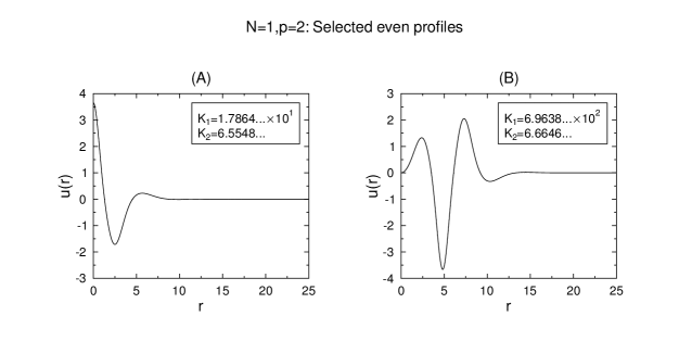
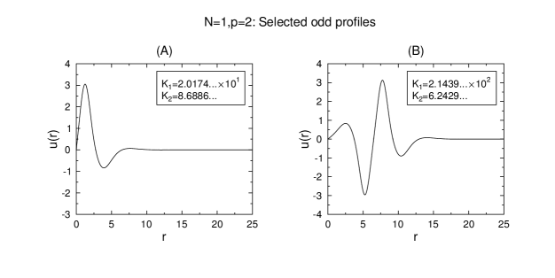
5. Numerical analysis in 1D and in the radial geometry
Considering radial geometry as discussed in section 2.1, (1.4) takes the form
| (5.1) |
This is considered together with the far-field asymptotic behaviour (2.3), written in the form
| (5.2) |
where we conveniently use the constants in place of , together with symmetry (2.4) or anti-symmetry (2.7) conditions at the origin.

Using the far-field behaviour (5.2), a 2-D shooting problem may be formulated where the parameters are determined by satisfying the symmetry condition (2.4) at the origin for the even profiles and anti-symmetry condition (2.7) for the odd profiles. Matlab’s ode15s solver is used with tight error tolerances (RelTol=AbsTol=).
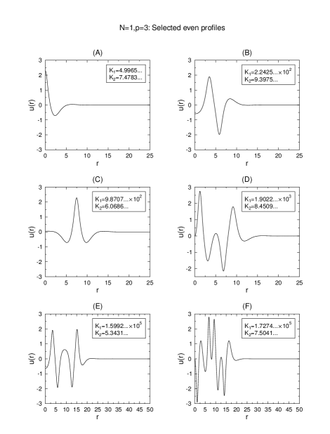
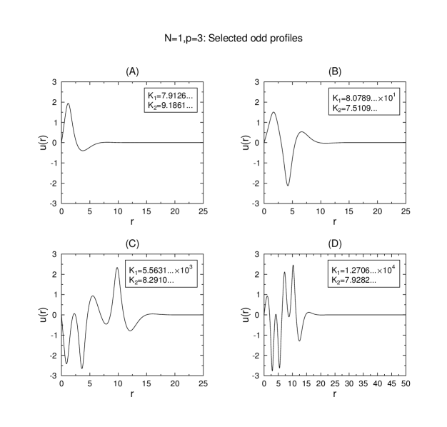
Figures 1–5 show illustrative even and odd profiles for and or . The condition (5.2) is used as initial data at sufficiently large (typically 25 or 50 as given by the domain in the plots).
We complete this numerical introduction with illustration of a different class of solutions to (5.1). We may perform numerical experiments, shooting smoothly from with and varying .

Shown in Figures 6 and 7 are selected profiles in one-dimension in the illustrative parameter cases and respectively. For sufficiently small seemingly chaotic patterns are obtained, which emerge into a more periodic structure as increases.

References
- [1] R.A. Adams and J.F. Fournier, Sobolev spaces. Second Edition. Pure and Applied Mathematics (Amsterdam), 140, Elsevier/Academic Press, Amsterdam (2003).
- [2] O.V. Admaev and V.V. Pukhnachev, Self-similar solutions of the equation , Preprint No. 3, Comp. Centre, Krasnoyarsk, 1997.
- [3] P. Álvarez-Caudevilla, Variational approach for a class of cooperative systems, Nonl. Anal. TMA, 75 (2012), 5620–5638.
- [4] P. Álvarez-Caudevilla, J.D. Evans, and V.A. Galaktionov, Countable families of solutions of a limit stationary semilinear fourth-order Cahn–Hilliard equation II. Non-Lusternik–Schnirel’man patterns in , in preparation.
- [5] P. Álvarez-Caudevilla and V.A. Galaktionov, Local bifurcation-branching analysis of global and “blow-up” patterns for a fourth-order thin film equation, Nonl. Differ. Equat. Appl., 18 (2011), 483–537.
- [6] P. Álvarez-Caudevilla and V.A. Galaktionov, Steady states, global existence and blow-up for fourth-order semilinear parabolic equations of Cahn–Hilliard type, Advances Nonl. Stud., 12 (2012), 315–361.
- [7] P. Álvarez-Caudevilla and J. López-Gómez, Asymptotic behavior of principal eigenvalues for a class of cooperative systems, J. Differ. Equat., 244 (2008), 1093–113.
- [8] H. Amann, Maximum principles and principal eigenvalues, In: Ten Mathematical Essays on Approximation in Analysis and Topology (J. Ferrera, J. López-Gómez, F.R. Ruiz del Portal, Eds.), Elsevier, Amsterdam, 2005, pp. 1–60.
- [9] A. Ambrosetti and P.H. Rabinowitz, Dual variational methods in critical point theory and applications, J. Funct. Anal., 14 (1973), 349–381.
- [10] M. Berger, Nonlinearity and Functional Analysis, Acad. Press, New York, 1977.
- [11] Haïm Brezis, Analyse fonctionnelle, Collection Mathématiques Appliquées pour la Maîtrise. [Collection of Applied Mathematics for the Master’s Degree], Masson, Paris, (1983), Théorie et applications. [Theory and applications].
- [12] J. Chabrowski and J. Marcos do Ó, On some fourth-order semilinear elliptic priblems in , Nonl. Anal., 49 (2002), 861–884.
- [13] M. Cross and H. Greenside Pattern formation and dynamics in nonequilibrium systems, CUP, New York, 2009.
- [14] J.D. Evans, V.A. Galaktionov, and J.F. Williams, Blow-up and global asymptotics of the limit unstable Cahn-Hilliard equation, SIAM J. Math. Anal., 38 (2006), 64–102.
- [15] J.D. Evans, V.A. Galaktionov, and J.R. King, Blow-up similarity solutions of the fourth-order unstable thin film equation, Euro. J. Appl. Math., 18 (2007), 195–231.
- [16] J.D. Evans, V.A. Galaktionov, and J.R. King, Source-type solutions of the fourth-order unstable thin film equation, Euro. J. Appl. Math., 18 (2007), 273–321.
- [17] D. G. de Figueiredo and E. Mitidieri, A maximum principle for an elliptic system and applications to semilinear problems, SIAM J. Math. Anal., 17 (1986), 836–849.
- [18] V.A. Galaktionov, E. Mitidieri, and S.I. Pohozaev, Variational approach to complicated similarity solutions of higher-order nonlinear evolution equations of parabolic, hyperbolic, and nonlinear dispersion types, In: Sobolev Spaces in Mathematics. II, Appl. Anal. and Part. Differ. Equat., Series: Int. Math. Ser., Vol. 9, V. Maz’ya Ed., Springer, New York, 2009 (an extended version in arXiv:0902.1425).
- [19] V.A. Galaktionov, E. Mitidieri, and S.I. Pohozaev, Variational approach to complicated similarity solutions of higher-order nonlinear PDEs. II, Nonl. Anal.: RWA, 12 (2011), 2435–2466 (arXiv:1103.2643).
- [20] V.A. Galaktionov and J.L. Vazquez, The problem of blow-up in nonlinear parabolic equations, Discr. Cont. Dyn. Syst., 8 (2002), 399–433.
- [21] Peter Hess, On the asymptotic distribution of eigenvalues of some nonselfadjoint problems, Bull. London Math. Soc., 18 (1986), 181–184.
- [22] R. Hoyle. Pattern formation. Cambridge University Press, 2006.
- [23] W. D. Kalies, J. Kwapisz and R.C.A.M. VanderVorst, Homotopy classes for stable connections between Hamiltonian saddle-focus equilibria, Comm. Math. Phys., 193 (1998), 337–371.
- [24] W. D. Kalies, J. Kwapisz, J.B. VandenBerg and R.C.A.M. VanderVorst, Homotopy classes for stable periodic and chaotic patterns in fourth-order Hamiltonian systems, Comm. Math. Phys., 214 (2000), 573–592 [Comm. Math. Phys., 215 (2001), 707–728].
- [25] G.A. Klassen and E. Mitidieri, Standing wave solutions for a system derived from the FitzHugh–Nagumo equations for nerve conduction, SIAM J. Math. Anal., 17 (1986), 74–83.
- [26] M.A. Krasnosel’skii, Topological Methods in the Theory of Nonlinear Integral Equations, Pergamon Press, Oxford/Paris, 1964.
- [27] M.A. Krasnosel’skii, Vector fields which are symmetric with respect to a subspace, Dokl. Acad. Nauk Ukrain. SSR, No. 1 (1951).
- [28] M.A. Krasnosel’skii and P.P. Zabreiko, Geometrical Methods of Nonlinear Analysis, Springer-Verlag, Berlin/Tokyo, 1984.
- [29] R.S. Laugesen and M.C. Pugh, Linear stability of steady states for thin film and Cahn–Hilliard type equations, Arch. Rat. Mech. Anal., 154 (2000), 3–51.
- [30] R.S. Laugesen and M.C. Pugh, Properties of steady states for thin film equations, Euro. J. Appl. Math., 11 (2000), 293–351.
- [31] R.S. Laugesen and M.C. Pugh, Energy levels of steady states for thin-film-type equations, J. Differ. Equat., 182 (2002), 377–415.
- [32] P.L. Lions, Symétrie et compacité dans les espaces de Sobolev. J. Funct. Anal. 49 (1982), no. 3, 315-334.
- [33] A. Novick-Cohen, Blow up and growth in the directional solidification of dilute binary alloys, Appl. Anal., 47 (1992), 241–257.
- [34] A. Novick-Cohen, The Cahn-Hilliard equation: mathematical and modeling perspectives, Adv. Math. Sci. Appl., 8 (1998), 965-=985.
- [35] A. Novick-Cohen, The Cahn-Hilliard equation, Handbook of Differential Equations: Evolutionary Equations, Vol. IV, 201–228, Handb. Differ. Equat., Elsevier/North-Holland, Amsterdam, 2008.
- [36] A. Novick-Cohen and L.A. Segel, Nonlinear aspects of the Cahn-Hilliard equation, Physica D, 10 (1984), 277-298.
- [37] M. Paniconi and K.R. Elder, Stationary, dynamical, and chaotic states of the two-dimensional Kuramoto-Sivashinsky equation, Physical Review E, 56 (1977), 2713-2721.
- [38] L.A. Peletier and W.C. Troy, Spatial Patterns. Higher Order Models in Physics and Mechanics, Birkhäusser, Boston/Berlin, 2001.
- [39] P.H. Rabinowitz, Minimax methods in critical point theory with applications to differential equations. CBMS Regional Conference Series in Mathematics, 65. Published for the Conference Board of the Mathematical Sciences, Washington, DC, Amer. Math. Soc., Providence, RI, 1986.
- [40] S. Santra and J. Wei, Homoclinic solutions for fourth order traveling wave equations, SIAM J. Math. Anal., 41 (2009), 2038–2056.
- [41] T. Sato and T. Watanabe, Singular positive solutions for a fourth order elliptic problem in , Commun. Pure Appl. Anal., 10 (2011), 245–268.
- [42] G. Talenti, Best Constant in Sobolev Inequality, Ann. Mat. Pura Appl., 110 (1976), 353–372.