Counterfactual Explainable Recommendation
Abstract.
By providing explanations for users and system designers to facilitate better understanding and decision making, explainable recommendation has been an important research problem. In this paper, we propose Counterfactual Explainable Recommendation (CountER), which takes the insights of counterfactual reasoning from causal inference for explainable recommendation. CountER is able to formulate the complexity and the strength of explanations, and it adopts a counterfactual learning framework to seek simple (low complexity) and effective (high strength) explanations for the model decision. Technically, for each item recommended to each user, CountER formulates a joint optimization problem to generate minimal changes on the item aspects so as to create a counterfactual item, such that the recommendation decision on the counterfactual item is reversed. These altered aspects constitute the explanation of why the original item is recommended. The counterfactual explanation helps both the users for better understanding and the system designers for better model debugging.
Another contribution of the work is the evaluation of explainable recommendation, which has been a challenging task. Fortunately, counterfactual explanations are very suitable for standard quantitative evaluation. To measure the explanation quality, we design two types of evaluation metrics, one from user’s perspective (i.e. why the user likes the item), and the other from model’s perspective (i.e. why the item is recommended by the model). We apply our counterfactual learning algorithm on a black-box recommender system and evaluate the generated explanations on five real-world datasets. Results show that our model generates more accurate and effective explanations than state-of-the-art explainable recommendation models. Source code is available at https://github.com/chrisjtan/counter.
1. Introduction
Explainability for recommender systems is crucial, because in recommendation scenarios we can rarely say that some recommendation is absolutely right or some other recommendation is absolutely wrong, instead, it all depends on good explanations to help users understand why an item is recommended so as to increase the transparency and trust and enable better decision making; good explanations also help system designers to track the behavior of the complicated recommendation models for better debugging (Zhang and Chen, 2020; Zhang et al., 2014a).
One prominent approach is aspect-aware explainable recommendation (Zhang et al., 2014a; Wang et al., 2018c; Chen et al., 2016, 2020b), which takes the explicit item features/aspects to construct explanations. For example, Zhang et al. (Zhang et al., 2014a) proposed Explicit Factor Model (EFM) which aligns latent factors with explicit features such as color and price to generate sentence explanations in the form of “You might be interested in [feature], on which this product performs well.” Wang et al. (Wang et al., 2018c) learned the user-aspect preferences in a multi-task joint tensor factorization framework to construct the aspect-aware explanations. Chen et al. (Chen et al., 2020b) explored attribute-aware collaborative filtering for explainable substitute recommendation. Li et al. (Li et al., 2021) proposed a Personalized Transformer to generate aspect-inspired natural language explanations. A more comprehensive review of related work is provided in Section 2.
However, existing methods on aspect-aware explainable recommendation face several issues: 1) Most of the methods are designed as intrinsic explainable models, although they have the advantage of providing faithful explanations, it may be difficult for them to explain other black-box recommendation models. 2) Existing methods do not consider the explanation complexity, in particular, they do not have the ability to decide how many aspects to use when generating explanations. Most methods generate explanations using exactly one aspect, however, the real reason of the recommendation may be triggered by multiple aspects. 3) Existing methods do not consider the explanation strength, i.e., to what extent the explanation really influences the recommendation result. This is mostly because existing methods are designed based on matching algorithms, which extracts associative signals such as feature importance and attention weights to construct explanations, while they seldom consider what happens if we intervene these signals to alternative values.
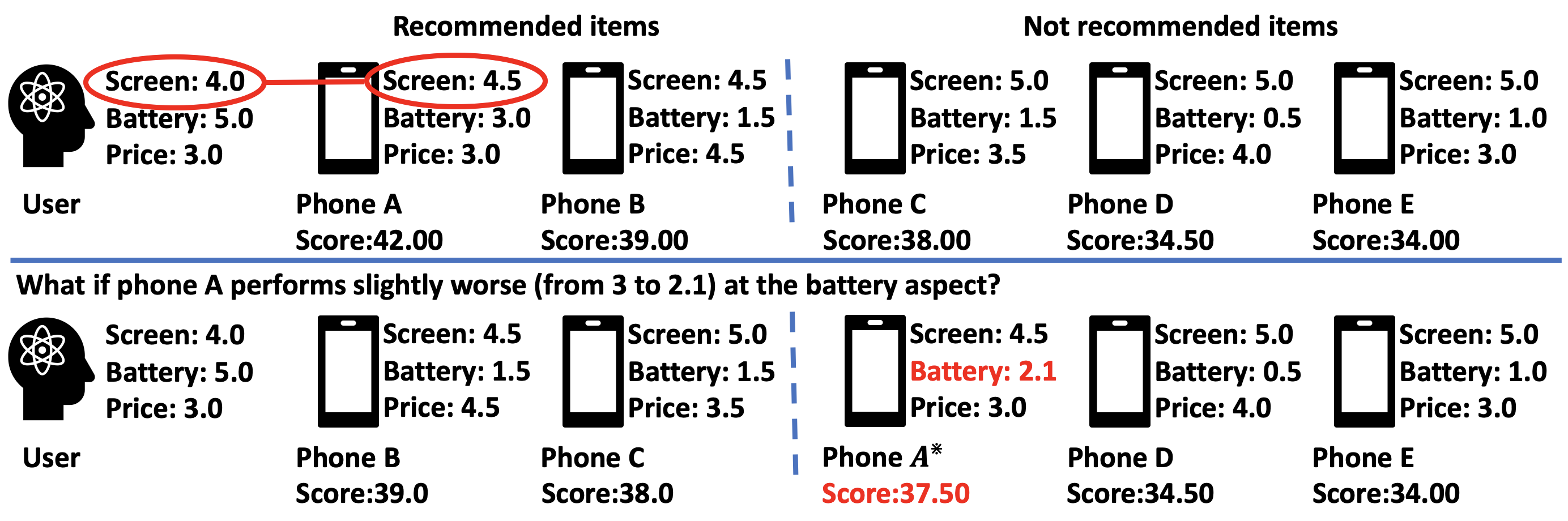
Recent advances on counterfactual reasoning shed light on the possibility to solve the above problems. We use a toy example in Figure 1 to illustrate the intuition of counterfactual explanation and its difference from matching-based explanation. In this example, similar to Zhang et al. (Zhang et al., 2014a), each user has his/her preference score on each aspect, while each item has its performance score on each aspect. The recommendation algorithm uses the total score to rank items. For example, the total score of Phone A is , which ranks at the 1st position of the recommendation list. To explain the recommendation of Phone A, a matching-based model would select screen as the explanation because the multiplication score for screen () is the highest compared to the other aspects ( for battery and for price). However, Phone A actually performs the worst on screen among all products, which makes this explanation unreasonable. This shows that the aspects with high matching scores may not always be the reason of the recommendation.
Counterfactual reasoning, on the contrary, aims to understand the underlying mechanism that really triggered the recommendation by applying interventions on the aspects and see what happens. As shown in the lower part of Figure 1, we can look for the minimal change on Phone A’s features such that Phone A will not be recommended anymore. In this case, the aspect battery will be selected as explanation because we only need to slightly change its score from 3 to 2.1 to reverse the recommendation decision, indicating that battery is a very influential factor on the recommendation result.
Following the above intuition, in this paper, we propose Counterfactual Explainable Recommendation (CountER), which adopts counterfactual reasoning to extract aspect-aware explanations for recommendation. Inspired by the Occam’s Razor Principle (Blumer et al., 1987), CountER is built on the fundamental idea of explanation complexity and explanation strength, where complexity measures how much change must be applied on the factual observations, and strength shows to what extent the applied change will influence the recommendation decision. Through our proposed counterfactual constrained learning framework, CountER aims to extract simple (low complexity) and effective (high strength) explanations for the recommendation by looking for minimal changes on the facts that would alter the recommendation decision.
Another important challenge in explainable recommendation (and explainable AI) research is how to evaluate the explanations. Due to the lack of standard offline evaluation measures for explanation, previous research heavily relied on human subjects for evaluation, which makes the evaluation process expensive, unscalable, hard to standardize, and unfriendly to academic research settings (Zhang and Chen, 2020). Fortunately, counterfactual explanations are very suitable for standard quantitative evaluation. In this paper, we propose two types of evaluation methods, one is user-oriented evaluation, and the other is model-oriented evaluation. For user-oriented evaluation, we adopt similar ideas as (Le and Lauw, 2020; Li et al., 2020, 2021) by using each user’s mentioned aspects in their reviews as the ground-truth. By comparing our generated explanation with the ground-truth, we can evaluate the feature coverage, precision, recall, and scores. For model-oriented evaluation, we adopt the Probability of Necessity (PN), Probability of Sufficiency (PS) and their harmonic mean to evaluate the sufficiency and necessity of the explanations. More details are provided in the experiments.
In summary, this work has the following contributions:
-
(1)
For the first time, we explore the complexity and the strength of explanations in explainable recommendation and formulate the concepts in mathematical ways.
-
(2)
We formulate a counterfactual reasoning framework based on counterfactual constrained learning to extract simple and effective explanations for recommendation.
-
(3)
We design both user-oriented and model-oriented metrics for standard evaluation of explainable recommendation.
-
(4)
We conduct extensive experiments on five real-world datasets to validate the effectiveness of our proposed method.
2. Related Work
In this section, we review some related work on explainable recommendation and counterfactual reasoning.
2.1. Explainable Recommendation
Explainable recommendation is a broad research area with many different types of models, and it is difficult to cover all of the works on this direction. Since our work is more closely related with aspect-aware explainable recommendation, we mainly focus on this sub-area in the section. A more complete review of explainable recommendation can be seen in (Zhang and Chen, 2020; Gedikli et al., 2014; Tintarev and Masthoff, 2015).
Explainability of recommender systems is important because it improves the transparency, user satisfaction and trust over the recommendation system (Zhang and Chen, 2020). One representative way to generate user-friendly explanations is by modeling aspects in the recommended items. For instance, Zhang et al. (Zhang et al., 2014a) introduced an Explicit Factor Model (EFM) for explainable recommendation. It first extracts the item aspects and the user opinions on these aspects from user reviews. Then, it trains a matrix factorization-based recommendation model to generate aspect-aware explanations by aligning the latent factors with the item aspects. Chen et al. (Chen et al., 2016) and Wang et al. (Wang et al., 2018c) advanced from matrix factorization to tensor factorization models for explainable recommendation. He et al. (He et al., 2015) proposed a tripartite graph model to improve the interactivity of aspect-aware recommendation models. Gao et al. (Gao et al., 2019) proposed an explainable deep model to learn multi-level user profile and infer which level of features best captures a user’s interest. Balog et al. (Balog et al., 2019) presented a set-based recommendation technique to improve the scrutability and transparency of recommender systems. Ren et al. (Ren et al., 2017) proposed a collaborative viewpoint regression for explainable social recommendation. Wang et al. (Wang et al., 2018b) proposed a tree-enhanced embedding method to combine embedding-based and tree-based models for explainable recommendation. More recently, Chen et al. (Chen et al., 2020b) applied a residual feed-forward neural network to model the user and item explicit features and generates explainable substitute recommendations. Pan et al. (Pan et al., 2020) presented a feature mapping approach to map the latent features onto the interpretable aspects to achieve both satisfactory accuracy and explainability. Li et al. (Li et al., 2021) proposed a Personalized Transformer to generate aspect-inspired natural language explanations. Xian et al. (Xian et al., 2021) developed an attribute-aware algorithm for explainable item-set recommendation and deployed in Amazon. Some other explainable recommendation methods include knowledge graph-based explanations (Xian et al., 2019, 2020; Ai et al., 2018), neural logic explanations (Zhu et al., 2021), visual explanations (Chen et al., 2019b), natural language explanations (Li et al., 2020; Chen et al., 2019a; Li et al., 2021; Li et al., 2017), dynamic explanations (Chen et al., 2019d), reinforcement learning-based explanations (Wang et al., 2018a), conversational explanations (Chen et al., 2020a; Zhao et al., 2019), fair explanations (Fu et al., 2020), disentangled explanations (Ma et al., 2019), review-based explanations (Chen et al., 2018; Ni et al., 2019), etc.
Most of the existing approaches generate explanations based on a very similar hypothesis: If there exists an aspect that best matches between the user’s preference and the item’s performance, then this aspect would be the explanation of the recommendation. However, our method generates explanations from a counterfactual perspective: if an item would not have been recommended had it performed slightly worse on some aspects, then these aspects would be the reason for the model to recommend this item.
2.2. Counterfactual Reasoning
Counterfactual reasoning, together with logical reasoning (Shi et al., 2020; Chen et al., 2021), are two important types of cognitive reasoning approaches. Recently, counterfactual reasoning has drawn attention in explainable AI research. It has some successful applications in several machine learning fields such as computer vision (Goyal et al., 2019), natural language processing (Hendricks et al., 2018; Feder et al., 2020), and social fairness (Wachter et al., 2018; Dandl et al., 2020). In the recommendation field, recent works used counterfactual reasoning to improve both recommendation accuracy (Wang et al., 2021; Xu et al., 2021a) and explainability (Ghazimatin et al., 2020; Xu et al., 2021b; Tran et al., 2021) based on heterogeneous information networks (Ghazimatin et al., 2020), perturbation model (Xu et al., 2021b) or influence functions (Tran et al., 2021), e.g., Ghazimatin et al. (Ghazimatin et al., 2020) tried to generate provider-side counterfactual explanations by looking for a minimal set of user’s historical actions (e.g. reviewing, purchasing, rating) such that the recommendation can be changed by removing the selected actions. Tran et al. (Tran et al., 2021) adopted influence functions for identifying training points most relevant to a recommendation while deducing a counterfactual set for explanations.
A common factor between our work with prior work is that both of the proposed methods generate explanations based on extracted causalities rather than associative relationships. Yet, our work is different from prior works on two key points: 1) In terms of problem definition, prior works generate counterfactual explanations on the user-side based on user actions while our method generates counterfactual explanations on the item-side based on item aspects, which are two different types of explanations. 2) In terms of technique, our method adopts a counterfactual learning framework driven by the Occam’s Razor Principle (Blumer et al., 1987) to directly learn an explanation of small complexity and large strength, so that our desire of finding simple and effective explanation is directly encoded into the model objective.
3. Problem Formulation
In this section, we first describe the preliminaries and the counterfactual explainable recommendation problem. Then, we introduce the concepts of explanation complexity, explanation strength, and their relations. Finally, we introduce the intuition of counterfactual reasoning. We leave the more formal and mathematical definition of our counterfactual reasoning framework to the next section.
3.1. Preliminaries and Notations
Suppose we have a user set with users and an item set with items . Let binary matrix be the user-item interaction matrix, where if user interacted with item ; otherwise, . We use to represent the top- recommendation list for a user , and we say if item is recommended to user in the user’s top- list. Following the same method described in Zhang et al. (Zhang et al., 2014a), we apply the sentiment analysis toolkit111https://github.com/evison/Sentires/ built in (Zhang et al., 2014b) to extract (Aspect, Opinion, Sentiment) triplets from the textual reviews. For example, in the Cell Phone domain, the extracted aspects would include color, price, screen, battery, etc. Besides, suppose we have a total number of item aspects . Same as (Zhang et al., 2014b), we further compute the user-aspect preference matrix and the item-aspect quality matrix . indicates to what extent the user cares about the item aspect . Similarly, indicates how well the item performs on the aspect . More specifically, and are calculated as:
| (1) | ||||
where is the rating scale in the system, which is 5-star in most cases. is the frequency that user mentioned aspect . is the frequency that item is mentioned on aspect , while is the average sentiment of these mentions. For both the and matrices, their elements are re-scaled into the range of using the sigmoid function (see Eq.(1)) to match with the system’s rating scale. Since the matrix construction process is not the focus of this work, we only briefly describe this process and readers may refer to (Zhang et al., 2014b, a) for more details. The same user-aspect and item-aspect matrix construction technique is also used in (Wang et al., 2018c; Gao et al., 2019; Le and Lauw, 2021).
3.2. Counterfactual Explainable Recommendation
With the above definitions, the objective of our counterfactual reasoning problem is to search for aspect-driven counterfactual explanations for a given black-box recommendation model.
More specifically, for a given recommendation model, if item is recommended to user , i.e., , then we look for a slight change vector for the item-aspect quality vector , such that if is applied on item ’s quality vector, i.e., , then it will change the recommendation result to make item disappear from the recommendation list, i.e., . All the values in are either zero or negative continuous values since an item will only be removed from the recommendation list if it performs worse on some aspects. With the optimized vector , we can construct the counterfactual explanation for item , which is composed of the aspects corresponding to the non-zero values in . The counterfactual explanation takes the following form, If the item had been slightly worse on [aspect(s)], then it will not be recommended. where the [aspect(s)] are selected by as mentioned above. In the following, we will define the properties of in more formal ways.
3.3. Explanation Complexity and Strength
To better understand the counterfactual explainable recommendation problem, we introduce two concepts to motivate explainable recommendation under the counterfactual reasoning background.
The first is Explanation Complexity (EC), which measures how complicated the explanation is. In our aspect-based explainable recommendation setting, the complexity can be defined as 1) how many aspects are used to generate the explanation, which corresponds to the number of non-zero values in , i.e., , and 2) how many changes need to be applied on these aspects, which can be represented as the sum of square of , i.e., . The final complexity takes a weighted sum of the two factors:
| (2) |
where is a hyper-parameter to control the trade-off between these two terms.
The second is Explanation Strength (ES), which measures how effective the explanation is. In our counterfactual explainable recommendation setting, this can be defined as to what extent applying the slight change vector will influence the recommendation result of item . This can be further defined as the decrease of ’s ranking score in user ’s recommendation list after applying :
| (3) |
where is the original ranking score of item , and is the ranking score of after is applied to its quality vector, i.e., .
We should note that Eq.(2) and (3) are not the only way to define explanation complexity and strength. The definition depends on what we need in practice. Our counterfactual reasoning framework introduced in Section 4 is flexible and can easily adapt to different definitions of explanation complexity and strength.
It is also worth discussing the relationship between explanation complexity and strength. Actually, complexity and strength are two orthogonal concepts, i.e., a complex explanation is not necessarily strong, and a simple explanation is not necessarily weak. There may well exist explanations that are complex but weak, or simple and strong. According to the Occam’s Razor Principle (Blumer et al., 1987), if two explanations are equally effective, we prefer the simpler explanation than the complex one. As a result, counterfactual explainable recommendation aims to seek the simple (low complexity) and effective (high strength) explanations for recommendation.
4. Counterfactual Reasoning
In this section, we first briefly introduce the black-box recommendation model for which we want to generate explanations. Then, we describe the details of our counterfactual constrained learning framework for counterfactual explainable recommendation.
4.1. Black-box Recommendation Model
Suppose we have a black-box recommendation model that predicts the user-item ranking score for user and item by:
| (4) |
where and are the user-aspect vector and item-aspect vector, respectively, as defined in Eq.(1); is the model parameter, and represents all other auxiliary information of the model. Depending on the application, could be ratings, clicks, text, images, etc., and is optional in the recommendation model. Basically, the recommendation model can be any model as long as it takes the user’s and the item’s aspect vectors as part of the input, which makes our counterfactual reasoning framework applicable to a wide scope of models.
In this work, to demonstrate the idea of counterfactual reasoning, we use a very simple deep neural network as the implementation of the recommendation model , which includes one fusion layer followed by three fully connected layers. The network concatenates the user’s and the item’s aspect vectors as input and outputs a one-dimensional ranking score . The final output layer is a sigmoid activation function so as to map into the range of . Then, we train the model with a cross-entropy loss:
| (5) |
where if user previously interacted with item , otherwise . In practice, since is a very sparse matrix, we sample the negative samples with ratio 1:2, i.e., for each positive instance we sample two negative instances. With this pre-trained recommendation model, for a target user, we are able to recommend top- items according to the predicted ranking scores.
4.2. Counterfactual Reasoning
We build a counterfactual reasoning model to generate explanations for any item in the top- recommendation list provided by an existing recommendation model. The essential idea of the proposed explanation model is to discover slight change on the item’s aspects via solving a counterfactual optimization problem which is formulated in the following.
Suppose item is in the top- recommendation list for user (). As mentioned before, our counterfactual reasoning model aims to find simple and effective explanations for , which can be shown as the following constrained optimization framework,
| (6) | Explanation Complexity | |||
| s.t., | Explanation is Strong Enough |
Mathematically, according to our definition of explanation complexity and strength in Section 3, the framework can be realized with the following specific optimization problem,
| (7) | ||||
where , . In the above equation, is the original ranking score of item , is the ranking score of when the slight change vector is applied on ’s aspect vector. The intuition of Eq.(7) is trying to find an explanation that is both simple and effective, where “simple” is reflected by the optimization objective, i.e., explanation complexity is minimized, while “effective” is reflected by the optimization constraint, i.e., the explanation strength should be big enough to remove item from the top- list.
To realize the second goal (i.e., effective/strong enough), we take the threshold as the margin between item ’s score and the ’s item’s score in the original recommendation list, i.e.,
| (8) |
where is the ranking score of the ’s item, and thus Eq.(7) can be simplified as,
| (9) | ||||
In this way, item will be ranked lower than the ’s item and thus be removed from the top- list.
4.3. Relaxed Optimization
A big challenge to optimize Eq.(9) is that both the objective and the constraint are not differentiable. In the following, we relax the two parts to make the equation optimizable.
For the objective, since is not convex, we relax it with -norm . This is shown to be efficient and provides good vector sparsity in (Candès et al., 2006; Candes and Tao, 2005), thus helps to minimize the explanation complexity in terms of the number of aspects in the explanation.
For the constraint , we relax it as a hinge loss:
| (10) |
and add it as a Lagrange term into the total objective. Thus, the final optimization equation for generating explanation becomes:
| (11) |
In Eq.(11), and are hyper-parameters to control the explanation strength. A sacrifice of using relaxed optimization is that we lose the guarantee that item is removed from the top- list, though the probability of removing is high due to minimizing the term. As a result, it requires a post-process to check if is indeed smaller than . We should only generate counterfactual explanations when the removal is successful. In the experiments, we will report the fidelity of our explanation model to show what percentage of items can be explained by our method.
Besides, there is a trade-off in the relaxed model: by increasing the hyper-parameter , the model will focus more on the explanation strength but less on the explanation complexity. We will also explore the influence of and the relationship between explanation complexity and strength in the ablation study of the experiments.
4.4. Discussions
4.4.1. Explanation Complexity for Items at Different Positions
With the above framework, we can see that the difficulty of removing different items in the top- list are different. Suppose for a certain user, the recommender system generates top- recommended items as according to the ranking scores. Intuitively, removing from the list is more difficult than removing from the list. The reason is that to remove , the explanation strength should be at least , which is bigger than the strength needed for removing , which is . As a result, the generated explanations for the items at a higher position in the list will likely have higher explanation complexity, because the reasoning model has to apply larger changes or more aspects to generate high-strength explanations.
This is a reasonable and desirable property of the counterfactual explainable recommendation framework—if the system ranks an item at a very high position, then it means that the system strongly recommends this item, which needs to be backed by strong explanation that contains more aspects. On the contrary, for an item ranked at lower positions in the list, it could be easily removed by changing only one or two aspects, which is in line with our intuition. In the experiments, we will show the average explanation complexity for items at different positions to verify the above discussion.
4.4.2. Controlling the Number of Aspects
Through Eq.(11), the model can automatically decide the number of aspects to construct the explanation. We believe this is better than choosing only one aspect as was done in previous aspect-aware explainable recommender systems (Zhang et al., 2014b; He et al., 2015; Wang et al., 2018c; Chen et al., 2020b). However, if needed, our method can also generate explanations with a single aspect. To generate single aspect explanation, we adjust Eq.(11) by adding a trainable one-hot vector a as a mask to make sure that only one aspect is changed during the training. The optimization problem is:
| (12) |
Since we force the model to generate single aspect explanation, the -norm term of vanishes because . We will explore both single- and multi-aspect explanations in experiment.
5. Evaluating Explanations
How to quantitatively evaluate explanations is a very important problem. Fortunately, compared to other explanation forms, counterfactual explanation is very suitable for quantitative offline evaluation. In this section, we mathematically define two types of evaluation metrics—user-oriented evaluation and model-oriented evaluation, which we believe can help the field to move forward with standard evaluation of explainable recommendations.
5.1. User-oriented Evaluation
In user-oriented evaluation, we adopt the user’s review on the item as the ground-truth reason about why the user purchased the item, which is similar to previous works (Li et al., 2020; Wang et al., 2018c; Li et al., 2017; Chen et al., 2019c, 2018). More specifically, from the textual review that a user provided on an item , we extract all the aspects that mentioned with positive sentiment, which is defined as . is a binary vector, where if user has positive sentiment on the aspect in his/her review for item . Otherwise, . On the other hand, our model will produce the vector , and those aspect(s) corresponding to the non-zero values in will constitute the explanation.
Then, for each user-item pair, we calculate the precision and recall of the generated explanation with regard to the ground-truth vector :
| (13) |
where is an identity function such that when , and when . In our case, the Precision measures the percentage of aspects in our generated explanation that are really liked by the user, while Recall measures how many percentage of aspects liked by the user are really included in our explanation. We also calculate the score as the harmonic mean between the two, i.e., . Then, we average the scores of all pairs as the final Precision, Recall, and measure.
5.2. Model-oriented Evaluation
The user-oriented evaluation only answers the question of whether the generated explanations are consistent with user’s preferences. However, it does not tell us whether the explanation properly justifies the model’s behaviour, i.e., why the recommendation model recommends this item to the user.
To test if our explanation model correctly explains the essential mechanism of the recommendation system, we use two scores, Probability of Necessity (PN) and Probability of Sufficiency (PS) (Pearl et al., 2016, p.112), to validate the explanations with model-oriented evaluation.
In logic and mathematics, necessity and sufficiency are terms used to describe a conditional or implicational relationship between two statements. Suppose we have , i.e., if happens then will happen, then we say is a sufficient condition for . Meanwhile, we have the logically equivalent contrapositive , i.e., if does not happen, then will not happen, as a result, we say is a necessary condition for .
Probability of Necessity (PN) (Pearl et al., 2016): In causal inference theory, probability of necessity evaluates the extent that a condition is necessary. To calculate PN for the generated explanation, suppose a set of aspects compose the explanation for the recommendation of item to user . The essential idea of the PN score is: if in a counterfactual world, the aspects in did not exist in the system, then what is the probability that item would not be recommended for user .
Following this idea, we calculate the frequency of the generated explanations that meet the PN definition. Let be user ’s original recommendation list. Let be a recommended item that our framework generated a nonempty explanation . Then for all the items in the universal item set , we alter the aspect values in the item-aspect quality matrix to 0 if they are in . In this way, we create a counterfactual item set which results in a counterfactual recommendation list for user by the recommendation algorithm. Then, the PN score is:
| (14) |
where is an identity function such that if the condition holds and 0 otherwise. Basically, the denominator is the total number of items that the algorithm successfully generated an explanation for, and the numerator is the number of explanations that if we remove the related aspects then it will cause the item to be removed from the recommendation list.
Probability of Sufficiency (PS) (Pearl et al., 2016): The PS score evaluates the extent that a condition is sufficient. The essential idea of the PS score is: if in a counterfactual world, the aspects in were the only aspects existed in the system, then what is the probability that item would still be recommended for user .
Similarly, we calculate the frequency of the generated explanations that meet the PS definition. For all the items in , we alter the aspect values in the item-aspect quality matrix to 0 if they are not in . In this way, we create a counterfactual item set which results in a counterfactual recommendation list for user by the recommendation algorithm. Then, the PS score is:
| (15) |
where is still the identity function as above. Basically, the denominator is still the total number of items that the algorithm successfully generated an explanation for, and the numerator is the number of explanations that alone can still recommend the item to the recommendation list. Similar to the user-oriented evaluation, we also calculate the harmonic mean of PS and PN to measure the overall performance, which is .
6. Experiments
In this section, we first introduce the datasets, the comparison baselines and the implementation details. Then we present studies on the two main expected properties in this paper: complexity and strength of the explanations. We also present ablation studies to explore how our model performs under different conditions.
6.1. Dataset Description
We test our method on Yelp222https://www.yelp.com/dataset and Amazon333https://nijianmo.github.io/amazon datasets. The Yelp dataset contains users’ reviews on various kinds of businesses such as restaurants, dentists, salons, etc. The Amazon dataset (Ni et al., 2019) contains user reviews on products in Amazon e-commerce system. The Amazon dataset contains 29 sub-datasets corresponding to 29 product categories. We adopt four datasets of different scales to evaluate our method, which are Electronic, Cell Phones and Accessories, Kindle Store and CDs and Vinyl. Since the Yelp and Amazon datasets are very sparse, similar as previous work (Zhang et al., 2014a; Wang et al., 2018c; Xian et al., 2019, 2020), we remove the users with less than 20 reviews for Yelp dataset, and 10 reviews for Amazon dataset. The statistics of the datasets are shown in Table 1.
6.2. Comparable Baselines
We compare our model with three aspect-aware explainable recommendation models. We also include a random explanation baseline to show the overall difficulty of the evaluation tasks.
EFM (Zhang et al., 2014a): The Explicit Factor Model. This work combines matrix factorization with sentiment analysis technique to align latent factors with explicit aspects. In this way, it predicts the user-aspect preference scores and item-aspect quality scores. The top-1 aligned aspect is used to construct aspect-based explanation.
MTER (Wang et al., 2018c): The Multi-Task Explainable Recommendation model. This work predicts a tensor , which represents the affinity score among the users, items, aspects, and an extra dimension for the overall rating. This tensor is acquired via Tucker decomposition (Karatzoglou et al., 2010; Kolda and Bader, 2009). We should note that since the overall rating for a user on an item is predicted in the extra dimension via decomposition, which is not directly predicted by the explicit aspects, this method is not suitable for the model-oriented evaluation. As a result, we only report this model’s explanation performance on user-oriented evaluation.
A2CF (Chen et al., 2020b): The Attribute-Aware Collaborative Filtering model. This work leverages a residual feed-forward network to predict the missing values in the user-aspect matrix and the item-aspect matrix . The method originally considers both the user-item preference and the item-item similarity to generate explainable substitute recommendations. We remove the item-item factor to make it compatible with our problem setting to generate explanations for any item. Similar to (Zhang et al., 2014a), the top-1 aligned aspect will be used for explanation.
Random: For each item recommended to a user, we randomly choose one or multiple aspects from the aspect space and generate the explanation based on them. The evaluation scores of the random baseline can indicate the difficulty of the task.
6.3. Implementation Details
6.3.1. Preprocessing
The preprocessing includes two parts: 1) Generating the user-aspect vector and the item-aspect vector from the user reviews. 2) Training the base recommender system. In the preprocessing phase, we hold-out the last 5 interacted items for each user, which serve as the test data to evaluate both the recommendation and the explanation. The deep neural network in the base recommendation model consists of fusion layer and fully connected layers with {, , } output dimensions, respectively. We apply ReLU activation function after all the layers except the last one, which is followed by a Sigmoid function to re-scale the predicted scores to the range of . The model parameters are optimized by stochastic gradient descent (SGD) optimizer with a learning rate of . After the recommendation model is trained, all the parameters will be fixed in the counterfactual reasoning phase and explanation evaluation phase.
| Dataset | #User | #Item | #Review | #Aspect | Density |
|---|---|---|---|---|---|
| Yelp | 11,863 | 20,181 | 497,252 | 106 | 0.208% |
| CDs and Vinyl | 8,119 | 52,193 | 245,391 | 230 | 0.058% |
| Kindle Store | 5,907 | 41,402 | 136,039 | 77 | 0.056% |
| Electronic | 2,832 | 19,816 | 53,295 | 105 | 0.095% |
| Cell Phones | 251 | 1,918 | 4,454 | 88 | 0.935% |
| Datasets | Single Aspect | Multiple Aspect | ||
|---|---|---|---|---|
| Mask | No Mask | Mask | No Mask | |
| Yelp | 61.60% | 62.54% | 79.30% | 86.38% |
| CDs and Vinyl | 41.52% | 75.84% | 93.80% | 94.20% |
| Kindle Store | 93.72% | 94.76% | 100.00% | 100.00% |
| Electronic | 63.32% | 70.52% | 81.80% | 98.00% |
| Cell Phones | 69.33% | 74.26% | 85.20% | 99.92% |
| Single Aspect Explanation | |||||||||||||||
| Electronic | Cell Phones | Kindle Store | CDs and Vinyl | Yelp | |||||||||||
| Pr% | Re% | F1% | Pr% | Re% | F1% | Pr% | Re% | F1% | Pr% | Re% | F1% | Pr% | Re% | F1% | |
| Random | 0.64 | 0.48 | 0.53 | 1.27 | 0.53 | 0.74 | 1.76 | 1.33 | 1.45 | 0.00 | 0.00 | 0.00 | 1.09 | 1.09 | 1.09 |
| EFM(Zhang et al., 2014a) | 24.58 | 16.52 | 18.79 | 20.01 | 15.33 | 17.98 | 39.25 | 34.37 | 35.96 | 36.36 | 20.00 | 24.24 | 7.18 | 7.18 | 7.18 |
| MTER(Wang et al., 2018c) | 23.90 | 17.45 | 19.32 | 20.83 | 11.35 | 14.06 | 31.23 | 27.31 | 28.54 | 15.52 | 13.79 | 14.37 | 6.17 | 6.17 | 6.17 |
| A2CF(Chen et al., 2020b) | 32.91 | 23.35 | 26.88 | 34.29 | 17.71 | 22.38 | 39.38 | 35.30 | 36.59 | 33.33 | 21.67 | 24.81 | 6.33 | 6.33 | 6.33 |
| CountER | 31.58 | 23.22 | 25.60 | 25.00 | 17.40 | 19.62 | 40.45 | 35.71 | 37.24 | 25.86 | 17.30 | 19.83 | 12.73 | 12.73 | 12.73 |
| CountER (w/ mask) | 33.94 | 25.67 | 28.31 | 29.21 | 20.26 | 22.85 | 40.94 | 36.19 | 37.73 | 39.06 | 25.93 | 29.33 | 12.96 | 12.96 | 12.96 |
| Multiple Aspect Explanation | |||||||||||||||
| Electronic | Cell Phones | Kindle Store | CDs and Vinyl | Yelp | |||||||||||
| Pr% | Re% | F1% | Pr% | Re% | F1% | Pr% | Re% | F1% | Pr% | Re% | F1% | Pr% | Re% | F1% | |
| Random | 0.19 | 0.75 | 0.30 | 1.43 | 2.87 | 1.46 | 1.79 | 1.75 | 1.74 | 0.39 | 0.68 | 0.49 | 1.06 | 3.54 | 1.62 |
| EFM(Zhang et al., 2014a) | 19.80 | 56.56 | 27.48 | 12.53 | 30.48 | 17.81 | 30.47 | 85.81 | 43.39 | 17.39 | 32.94 | 20.50 | 5.32 | 9.76 | 6.70 |
| MTER(Wang et al., 2018c) | 10.54 | 27.24 | 13.42 | 12.50 | 25.00 | 16.67 | 12.93 | 40.16 | 18.90 | 14.41 | 39.28 | 19.74 | 5.32 | 15.93 | 7.56 |
| A2CF(Chen et al., 2020b) | 18.07 | 53.72 | 25.32 | 16.05 | 28.29 | 18.76 | 31.86 | 80.44 | 43.27 | 19.39 | 57.84 | 26.62 | 4.58 | 16.67 | 7.00 |
| CountER | 17.42 | 45.72 | 22.13 | 19.13 | 47.70 | 25.05 | 27.79 | 86.07 | 40.68 | 16.21 | 33.55 | 19.96 | 6.67 | 23.73 | 10.18 |
| CountER (w/ mask) | 25.68 | 45.78 | 29.73 | 21.72 | 42.82 | 26.97 | 32.24 | 84.20 | 44.57 | 20.95 | 68.98 | 30.00 | 9.09 | 28.57 | 13.57 |
6.3.2. Generating Explanations
The base recommendation model generates the top- recommendation list for each user. is set to in the experiment. We then apply the counterfactual reasoning method to generate explanations for the items in the list. The hyper-parameter is set to 100 for all the datasets. The ablation study on the influence of can be seen in Section 6.5. We notice that the -norm and the -norm is almost in the same scale, so that we always set to 1 in our model. For the margin value in the hinge loss, we tested different values for in and find that the performance does not change too much for and then significantly drops for . As a result, we set throughout the experiments. To compare with the baselines, for each recommended item, we generate both multi-aspect and single-aspect explanation through Eq.(11) and Eq.(12), respectively.
6.3.3. Aspect Masking
When generating explanations, our model directly chooses aspects from the entire aspect space, which is reflected by the change vector . However, in the user-oriented evaluation, a strong bias exists in the user’s ground-truth review, which is that a user is more possible to mention the aspects that they have mentioned before. This may result from the personal linguistic preferences. As a result, all the baseline models (EFM, MTER, A2CF) only choose aspects from the user’s previously mentioned aspects to construct the explanation. To fairly compare with them in the user-oriented evaluation, we provide an adjusted version of our model. Let be the user ’s mask vector. is a binary vector, where if aspect is an aspect that cares about, i.e., . Otherwise, . We apply this mask on to generate explanation by choosing aspects only from the user’s preference space. which is:
| (16) |
In this case, the is used to generate explanation. This aspect mask can also be applied on the single-aspect formula, i.e., . Notice that applying the mask does not introduce the data leakage problem because the mask is calculated based on the training set. In the evaluation, we evaluate both the original CountER model and the masked CountER model in both user-oriented and model-oriented evaluations.
6.3.4. Compatible with the Baselines
One issue in comparison with baselines is that our model is able to generate both multi-aspect and single-aspect explanations. When generating multi-aspect explanations, the model automatically decides the best number of aspects in model learning. However, the baseline methods can only generate single-aspect explanations using the top-1 aligned aspect since they do not have the ability to decide the number of aspects. Thus, to make the baseline models also comparable in multi-aspect explanation, we use our model as a guideline to tell the baseline models how many aspects should they use to generate multi-aspect explanations. For this reason, we only compare the explanations generated for the intersection of the items which are recommended by both our model and the baseline models in multi-aspect setting.
6.3.5. Evaluable Explanations
Even if the explanation model can generate explanations for all the recommended items, not all of the explanations can be evaluated from the user’s perspective. This is because the user-oriented evaluation requires the user reviews as the ground-truth data. Thus, we can only evaluate the explanations generated for the “correctly recommended” items which appear in the test data. For model-oriented evaluation, all the explanations can be evaluated.
| Single Aspect Explanation | |||||||||||||||
| Electronic | Cell Phones | Kindle Store | CDs and Vinyl | Yelp | |||||||||||
| PN% | PS% | % | PN% | PS% | % | PN% | PS% | % | PN% | PS% | % | PN% | PS% | % | |
| Random | 2.05 | 2.10 | 2.07 | 3.39 | 3.50 | 3.44 | 3.16 | 2.75 | 2.94 | 1.58 | 2.03 | 1.78 | 7.52 | 10.68 | 8.82 |
| EFM(Zhang et al., 2014a) | 8.41 | 41.13 | 13.96 | 32.31 | 82.09 | 46.37 | 6.01 | 73.84 | 11.12 | 10.15 | 42.63 | 16.39 | 5.87 | 61.06 | 10.71 |
| A2CF(Chen et al., 2020b) | 41.45 | 77.60 | 54.03 | 36.82 | 78.68 | 50.17 | 25.66 | 65.53 | 36.88 | 25.41 | 84.51 | 39.07 | 17.59 | 96.92 | 29.78 |
| CountER | 65.54 | 68.28 | 66.83 | 74.03 | 63.30 | 68.25 | 34.37 | 41.50 | 37.60 | 49.62 | 54.72 | 52.04 | 65.26 | 53.25 | 58.64 |
| CountER (w/ mask) | 56.73 | 62.03 | 59.26 | 70.11 | 54.71 | 61.46 | 35.39 | 46.91 | 40.34 | 75.17 | 49.18 | 59.46 | 58.52 | 52.56 | 55.38 |
| Multiple Aspect Explanation | |||||||||||||||
| Electronic | Cell Phones | Kindle Store | CDs and Vinyl | Yelp | |||||||||||
| PN% | PS% | % | PN% | PS% | % | PN% | PS% | % | PN% | PS% | % | PN% | PS% | % | |
| Random | 2.24 | 4.90 | 3.08 | 6.25 | 10.13 | 7.73 | 5.80 | 7.80 | 6.65 | 3.22 | 7.65 | 4.53 | 13.84 | 12.92 | 13.36 |
| EFM(Zhang et al., 2014a) | 29.65 | 84.67 | 43.92 | 52.66 | 87.98 | 65.88 | 51.72 | 96.42 | 67.33 | 47.65 | 87.35 | 61.66 | 16.76 | 81.68 | 27.81 |
| A2CF(Chen et al., 2020b) | 59.47 | 81.66 | 68.82 | 56.45 | 80.97 | 66.52 | 52.48 | 87.59 | 65.64 | 49.12 | 91.52 | 63.93 | 41.38 | 98.28 | 58.24 |
| CountER | 97.08 | 96.24 | 96.66 | 99.52 | 98.48 | 99.00 | 64.00 | 79.20 | 70.79 | 80.89 | 88.60 | 84.57 | 99.91 | 94.12 | 96.93 |
| CountER (w/ mask) | 77.96 | 89.26 | 83.23 | 86.62 | 91.78 | 89.13 | 60.70 | 80.10 | 69.06 | 72.47 | 67.72 | 70.01 | 96.73 | 94.39 | 95.55 |
6.4. Experimental Results
We first report the fidelity of our explanation method in Table 2, which shows for what percentage of recommended items that our method can successfully generate an explanation. We notice that the fidelity of the single-aspect version is lower than that of the multi-aspect version. This indicates that for our model, using only one aspect as the explanation may not lead to enough explanation strength to effectively explain the recommendations. However, if we allow the model to use multiple aspects, we can find strong enough explanations in most cases (). The overall average number of aspects in multi-aspect explanation is .
We then evaluate the explanations generated by CountER (original version and masked version) and the baselines. The user-oriented evaluation is reported in Table 3 and the model-oriented evaluation is reported in Table 4. We note that the random baseline performs very bad on both evaluations, which shows the difficulty of the task and that randomly choosing aspects as explanations can barely reveal the reasons of the recommendations.
For the user-oriented evaluation, the results show that when applying the mask for fair comparison, CountER outperforms all the baselines on all the datasets in terms of scores. Moreover, CountER performs better than the baselines on precision in cases and on recall in cases. We note that our model has a very huge improvement than the baselines on Yelp dataset even without mask, and the reason may be that the Yelp dataset is much denser and has more reviews than other datasets so that the user’s review bias has smaller impact. This also indicates that CountER has more advantages when the size of dataset increases.
For model-oriented evaluation, the mask limits CountER’s ability to explain the model’s behavior. However, no matter with or without the mask, our model has better performance than all the baselines according to score. With mask, CountER has average improvement than the best performance of the baselines on . Without the mask, the average improvement is .
Another observation is that the baselines commonly have higher PS scores, despite much lower on the PN scores. One possible reason is due to the mechanism of the matching based explanation methods. For an item on the recommendation list, they try to find well-aligned aspects where the user and the item both perform well. When computing the PS score, the baselines only reserve these well-aligned aspects in the aspect space for all the items, thus the recommended item will highly possibly still stay in the recommendation list, which results in a high PS score. However, when computing the PN score, though the baselines remove all these aspects, the recommended item may still perform better on other aspects compared with other items and thus still remain in the recommendation list, which results in a lower PN score. This also sheds light on why the matching based methods may not discover the true reasons behind the recommendations.
6.5. Influence of Relaxation Weight
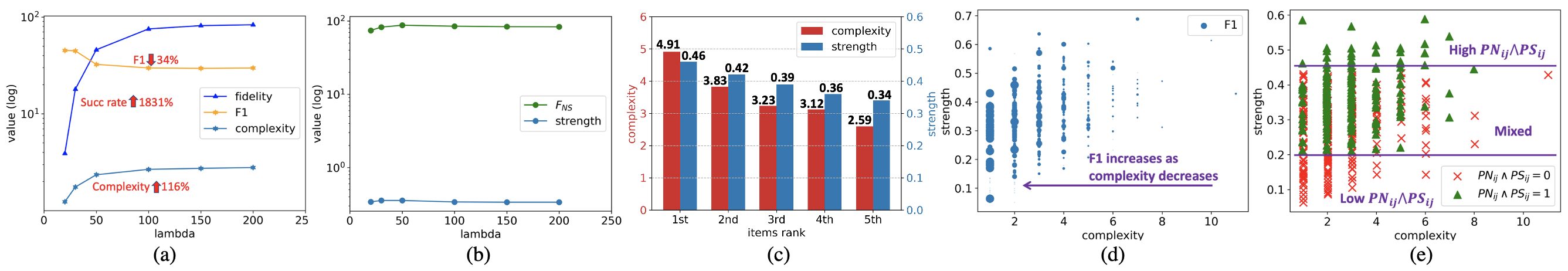
Since is applied on the hinge loss (Eq.(11) and (12)), a larger emphasizes more on the explanation strength and reduces the importance of complexity. As shown in Figure 2(a), when increases, the model successfully generates explanations for more items, but the explanation complexity also increases because more aspects are needed to explain those “hard” items. However, the higher is, the worse our model performs on the user-oriented evaluation. Besides, Figure 2(b) shows the explanation strength does not change with . This is because the in the hinge loss controls the required margin on the ranking score to flip a recommendation. Additionally, we notice that the model-oriented performance is also independent to , which is the same as the explanation strength.
Based on the above results, we hypothesize that the user-oriented performance may be related to the explanation complexity, while the model-oriented performance may be related to the explanation strength. This hypothesis is justified in Section 6.6.
6.6. Explanation Complexity and Strength
In this section, we study the Explanation Complexity and Explanation Strength. In Section 4.4.1, we discussed that the difficulty of removing the items in the top- list are different based on their positions. Figure 2(c) shows the mean complexity and strength of the explanations for items at different positions (i.e., from the first to the fifth). Generally speaking, it requires more aspects to remove the items at the first position from the recommendation list than the items at the fifth position. Because they require larger change to be removed. This is in line with the fact that the strongly recommended items have more reasons to be recommended.
In Figure 2(d), we illustrate the relationship between score and explanation complexity/strength. The scale of the marker points represent how large the score is. It shows that the user-oriented evaluation score decreases as the complexity increases, meanwhile, is relatively independent from the explanation strength.
On the contrary, in Figure 2(e), we plot the distribution of the explanations that are both necessary and sufficient (i.e., ), as well as the distribution of explanations that are either unnecessary or insufficient (i.e., ). We can see that as the explanation strength increases, more and more portion of the explanations are both necessary and sufficient. However, this tends to be irrelevant with the complexity of the explanations.
These observations are important because: 1) They indicate that the Explanation Complexity and Explanation Strength are two orthogonal concepts. Both of them are very important since the complexity is related to the coverage on the user’s preference and the strength is related to the model’s mechanism. 2) It legitimatizes the Occam’s Razor Principle and further justifies the motivation of our CountER model, which is to extract both simple (low complexity) and effective (high strength) explanations for recommendations.
7. Conclusions and Future Work
In this paper, we proposed CountER, a counterfactual explainable recommendation framework, which generates explanations based on counterfactual changes on item aspects. Counterfactual reasoning is still in early stages for explainable recommendation, which has a lot of room for further explorations. For instance, CountER only explored changes on the item aspects. However, we can also explore counterfactual changes on other various forms of information such as images and textual descriptions. The essential idea of CountER is also suitable for explainable decision making over knowledge graphs or graph neural networks, which are very promising directions to explore in the future.
Acknowledgments
We appreciate the valuable feedback and suggestions of the reviewers. This work was supported in part by NSF IIS-1910154 and IIS-2007907. Any opinions, findings, conclusions or recommendations expressed in this material are those of the authors and do not necessarily reflect those of the sponsors.
References
- (1)
- Ai et al. (2018) Qingyao Ai, Vahid Azizi, Xu Chen, and Yongfeng Zhang. 2018. Learning heterogeneous knowledge base embeddings for explainable recommendation. Algorithms.
- Balog et al. (2019) Krisztian Balog, Filip Radlinski, and Shushan Arakelyan. 2019. Transparent, scrutable and explainable user models for personalized recommendation. In SIGIR. 265–274.
- Blumer et al. (1987) Anselm Blumer, Andrzej Ehrenfeucht, David Haussler, and Manfred K Warmuth. 1987. Occam’s razor. Information processing letters 24, 6 (1987), 377–380.
- Candes and Tao (2005) E. J. Candes and T. Tao. 2005. Decoding by linear programming. IEEE Transactions on Information Theory 51, 12 (2005), 4203–4215.
- Candès et al. (2006) Emmanuel J. Candès, Justin K. Romberg, and Terence Tao. 2006. Stable signal recovery from incomplete and inaccurate measurements. Communications on Pure and Applied Mathematics 59, 8 (2006), 1207–1223.
- Chen et al. (2018) Chong Chen, Min Zhang, Yiqun Liu, and Shaoping Ma. 2018. Neural attentional rating regression with review-level explanations. In WWW. 1583–1592.
- Chen et al. (2019a) Hanxiong Chen, Xu Chen, Shaoyun Shi, and Yongfeng Zhang. 2019a. Generate natural language explanations for recommendation. SIGIR 2019 Workshop on ExplainAble Recommendation and Search (2019).
- Chen et al. (2021) Hanxiong Chen, Shaoyun Shi, Yunqi Li, and Yongfeng Zhang. 2021. Neural Collaborative Reasoning. In Proceedings of the Web Conference 2021. 1516–1527.
- Chen et al. (2020b) Tong Chen, Hongzhi Yin, Guanhua Ye, Zi Huang, Yang Wang, and Meng Wang. 2020b. Try this instead: Personalized and interpretable substitute recommendation. In SIGIR. 891–900.
- Chen et al. (2019b) Xu Chen, Hanxiong Chen, Hongteng Xu, Yongfeng Zhang, Yixin Cao, Zheng Qin, and Hongyuan Zha. 2019b. Personalized fashion recommendation with visual explanations based on multimodal attention network: Towards visually explainable recommendation. In SIGIR. 765–774.
- Chen et al. (2016) Xu Chen, Zheng Qin, Yongfeng Zhang, and Tao Xu. 2016. Learning to Rank Features for Recommendation over Multiple Categories. In SIGIR. 305–314.
- Chen et al. (2019d) Xu Chen, Yongfeng Zhang, and Zheng Qin. 2019d. Dynamic explainable recommendation based on neural attentive models. In AAAI, Vol. 33. 53–60.
- Chen et al. (2020a) Zhongxia Chen, Xiting Wang, Xing Xie, Mehul Parsana, Akshay Soni, Xiang Ao, and Enhong Chen. 2020a. Towards Explainable Conversational Recommendation.. In IJCAI. 2994–3000.
- Chen et al. (2019c) Zhongxia Chen, Xiting Wang, Xing Xie, Tong Wu, Guoqing Bu, Yining Wang, and Enhong Chen. 2019c. Co-Attentive Multi-Task Learning for Explainable Recommendation.. In IJCAI. 2137–2143.
- Dandl et al. (2020) Susanne Dandl, Christoph Molnar, Martin Binder, and Bernd Bischl. 2020. Multi-Objective Counterfactual Explanations. Lecture Notes in Computer Science (2020).
- Feder et al. (2020) Amir Feder, Nadav Oved, Uri Shalit, and Roi Reichart. 2020. CausaLM: Causal Model Explanation Through Counterfactual Language Models. arXiv:2005.13407
- Fu et al. (2020) Zuohui Fu, Yikun Xian, Ruoyuan Gao, Jieyu Zhao, Qiaoying Huang, Yingqiang Ge, Shuyuan Xu, Shijie Geng, Chirag Shah, Yongfeng Zhang, et al. 2020. Fairness-aware explainable recommendation over knowledge graphs. In SIGIR. 69–78.
- Gao et al. (2019) Jingyue Gao, Xiting Wang, Yasha Wang, and Xing Xie. 2019. Explainable recommendation through attentive multi-view learning. In AAAI, Vol. 33. 3622–3629.
- Gedikli et al. (2014) Fatih Gedikli, Dietmar Jannach, and Mouzhi Ge. 2014. How should I explain? A comparison of different explanation types for recommender systems. International Journal of Human-Computer Studies 72, 4 (2014), 367–382.
- Ghazimatin et al. (2020) Azin Ghazimatin, Oana Balalau, Rishiraj Saha Roy, and Gerhard Weikum. 2020. PRINCE: Provider-side Interpretability with Counterfactual Explanations in Recommender Systems. WSDM (2020).
- Goyal et al. (2019) Yash Goyal, Ziyan Wu, Jan Ernst, Dhruv Batra, Devi Parikh, and Stefan Lee. 2019. Counterfactual visual explanations. In ICML. 2376–2384.
- He et al. (2015) Xiangnan He, Tao Chen, Min-Yen Kan, and Xiao Chen. 2015. Trirank: Review-aware explainable recommendation by modeling aspects. In CIKM. 1661–1670.
- Hendricks et al. (2018) Lisa Anne Hendricks, Ronghang Hu, Trevor Darrell, and Zeynep Akata. 2018. Generating Counterfactual Explanations with Natural Language. arXiv:1806.09809
- Karatzoglou et al. (2010) Alexandros Karatzoglou, Xavier Amatriain, Linas Baltrunas, and Nuria Oliver. 2010. Multiverse recommendation: n-dimensional tensor factorization for context-aware collaborative filtering. In RecSys. 79–86.
- Kolda and Bader (2009) Tamara G Kolda and Brett W Bader. 2009. Tensor decompositions and applications. SIAM review 51, 3 (2009), 455–500.
- Le and Lauw (2020) Trung-Hoang Le and Hady W. Lauw. 2020. Synthesizing Aspect-Driven Recommendation Explanations from Reviews. In IJCAI. 2427–2434.
- Le and Lauw (2021) Trung-Hoang Le and Hady W Lauw. 2021. Explainable Recommendation with Comparative Constraints on Product Aspects. In WSDM. 967–975.
- Li et al. (2020) Lei Li, Yongfeng Zhang, and Li Chen. 2020. Generate neural template explanations for recommendation. In CIKM. 755–764.
- Li et al. (2021) Lei Li, Yongfeng Zhang, and Li Chen. 2021. Personalized Transformer for Explainable Recommendation. ACL (2021).
- Li et al. (2017) Piji Li, Zihao Wang, Zhaochun Ren, Lidong Bing, and Wai Lam. 2017. Neural rating regression with abstractive tips generation for recommendation. In SIGIR.
- Ma et al. (2019) Jianxin Ma, Chang Zhou, Peng Cui, Hongxia Yang, and Wenwu Zhu. 2019. Learning disentangled representations for recommendation. In NeurIPS. 5711–5722.
- Ni et al. (2019) Jianmo Ni, Jiacheng Li, and Julian McAuley. 2019. Justifying recommendations using distantly-labeled reviews and fine-grained aspects. In EMNLP. 188–197.
- Pan et al. (2020) Deng Pan, Xiangrui Li, Xin Li, and Dongxiao Zhu. 2020. Explainable recommendation via interpretable feature mapping and evaluation of explainability. IJCAI (2020).
- Pearl et al. (2016) Judea Pearl, Madelyn Glymour, and Nicholas P Jewell. 2016. Causal inference in statistics: A primer. John Wiley & Sons.
- Ren et al. (2017) Zhaochun Ren, Shangsong Liang, Piji Li, Shuaiqiang Wang, and Maarten de Rijke. 2017. Social collaborative viewpoint regression with explainable recommendations. In WSDM. 485–494.
- Shi et al. (2020) Shaoyun Shi, Hanxiong Chen, Weizhi Ma, Jiaxin Mao, Min Zhang, and Yongfeng Zhang. 2020. Neural logic reasoning. In CIKM. 1365–1374.
- Tintarev and Masthoff (2015) Nava Tintarev and Judith Masthoff. 2015. Explaining Recommendations: Design and Evaluation. In Recommender Systems Handbook (2 ed.). Chapter 10, 353–382.
- Tran et al. (2021) Khanh Hiep Tran, Azin Ghazimatin, and Rishiraj Saha Roy. 2021. Counterfactual Explanations for Neural Recommenders. SIGIR (2021), 1627–1631.
- Wachter et al. (2018) Sandra Wachter, Brent Mittelstadt, and Chris Russell. 2018. Counterfactual Explanations without Opening the Black Box: Automated Decisions and the GDPR. arXiv:1711.00399
- Wang et al. (2018c) Nan Wang, Hongning Wang, Yiling Jia, and Yue Yin. 2018c. Explainable Recommendation via Multi-Task Learning in Opinionated Text Data. SIGIR (2018).
- Wang et al. (2018a) Xiting Wang, Yiru Chen, Jie Yang, Le Wu, Zhengtao Wu, and Xing Xie. 2018a. A reinforcement learning framework for explainable recommendation. In ICDM.
- Wang et al. (2018b) Xiang Wang, Xiangnan He, Fuli Feng, Liqiang Nie, and Tat-Seng Chua. 2018b. Tem: Tree-enhanced embedding model for explainable recommendation. In WWW.
- Wang et al. (2021) Zhenlei Wang, Jingsen Zhang, Hongteng Xu, Xu Chen, Yongfeng Zhang, Wayne Xin Zhao, and Ji-Rong Wen. 2021. Counterfactual Data-Augmented Sequential Recommendation. In SIGIR. 347–356.
- Xian et al. (2019) Yikun Xian, Zuohui Fu, Shan Muthukrishnan, Gerard De Melo, and Yongfeng Zhang. 2019. Reinforcement knowledge graph reasoning for explainable recommendation. In SIGIR. 285–294.
- Xian et al. (2020) Yikun Xian, Zuohui Fu, Handong Zhao, Yingqiang Ge, Xu Chen, Qiaoying Huang, Shijie Geng, Zhou Qin, Gerard de Melo, S. Muthukrishnan, and Yongfeng Zhang. 2020. CAFE: Coarse-to-Fine Neural Symbolic Reasoning for Explainable Recommendation. In CIKM. 1645–1654.
- Xian et al. (2021) Yikun Xian, Tong Zhao, Jin Li, Jim Chan, Andrey Kan, Jun Ma, Xin Luna Dong, Christos Faloutsos, George Karypis, Shan Muthukrishnan, and Yongfeng Zhang. 2021. EX3: Explainable Attribute-aware Item-set Recommendations. In RecSys.
- Xu et al. (2021a) Shuyuan Xu, Yingqiang Ge, Yunqi Li, Zuohui Fu, Xu Chen, and Yongfeng Zhang. 2021a. Causal Collaborative Filtering. arXiv:2102.01868 (2021).
- Xu et al. (2021b) Shuyuan Xu, Yunqi Li, Shuchang Liu, Zuohui Fu, Yingqiang Ge, Xu Chen, and Yongfeng Zhang. 2021b. Learning Causal Explanations for Recommendation. The 1st International Workshop on Causality in Search and Recommendation (2021).
- Zhang and Chen (2020) Yongfeng Zhang and Xu Chen. 2020. Explainable Recommendation: A Survey and New Perspectives. Foundations and Trends® in Information Retrieval (2020).
- Zhang et al. (2014a) Yongfeng Zhang, Guokun Lai, Min Zhang, Yi Zhang, Yiqun Liu, and Shaoping Ma. 2014a. Explicit Factor Models for Explainable Recommendation Based on Phrase-Level Sentiment Analysis. In SIGIR. 83–92.
- Zhang et al. (2014b) Yongfeng Zhang, Haochen Zhang, Min Zhang, Yiqun Liu, and Shaoping Ma. 2014b. Do Users Rate or Review? Boost Phrase-Level Sentiment Labeling with Review-Level Sentiment Classification. In SIGIR. 1027–1030.
- Zhao et al. (2019) Guoshuai Zhao, Hao Fu, Ruihua Song, Tetsuya Sakai, Zhongxia Chen, Xing Xie, and Xueming Qian. 2019. Personalized reason generation for explainable song recommendation. ACM Transactions on Intelligent Systems and Technology (TIST) 10, 4 (2019), 1–21.
- Zhu et al. (2021) Yaxin Zhu, Yikun Xian, Zuohui Fu, Gerard de Melo, and Yongfeng Zhang. 2021. Faithfully Explainable Recommendation via Neural Logic Reasoning. In Proceedings of the 2021 Conference of the North American Chapter of the Association for Computational Linguistics: Human Language Technologies. 3083–3090.