Counterfactual Generation Under
Confounding
Abstract
A machine learning model, under the influence of observed or unobserved confounders in the training data, can learn spurious correlations and fail to generalize when deployed. For image classifiers, augmenting a training dataset using counterfactual examples has been empirically shown to break spurious correlations. However, the counterfactual generation task itself becomes more difficult as the level of confounding increases. Existing methods for counterfactual generation under confounding consider a fixed set of interventions (e.g., texture, rotation) and are not flexible enough to capture diverse data-generating processes. Given a causal generative process, we formally characterize the adverse effects of confounding on any downstream tasks and show that the correlation between generative factors (attributes) can be used to quantitatively measure confounding between generative factors. To minimize such correlation, we propose a counterfactual generation method that learns to modify the value of any attribute in an image and generate new images given a set of observed attributes, even when the dataset is highly confounded. These counterfactual images are then used to regularize the downstream classifier such that the learned representations are the same across various generative factors conditioned on the class label. Our method is computationally efficient, simple to implement, and works well for any number of generative factors and confounding variables. Our experimental results on both synthetic (MNIST variants) and real-world (CelebA) datasets show the usefulness of our approach.
1 Introduction
A confounder is a variable that causally influences two or more variables that are not necessarily directly causally dependent (Pearl, 2001). Often, the presence of confounders in a data-generating process is the reason for spurious correlations among variables in the observational data. The bias caused by such confounders is inevitable in observational data, making it challenging to identify invariant features representative of a target variable (Rothenhäusler et al., 2021; Meinshausen & Bühlmann, 2015; Wang et al., 2022). For example, the demographic area an individual resides in often confounds the race and perhaps the level of education that individual receives. Using such observational data, if the goal is to predict an individual’s salary, a machine learning model may exploit the spurious correlation between education and race even though those two variables should ideally be treated as independent variables. Removing the effects of confounding in trained machine learning models has shown to be helpful in various applications such as zero or few-shot learning, disentanglement, domain generalization, counterfactual generation, algorithmic fairness, healthcare, etc. (Suter et al., 2019; Kilbertus et al., 2020; Atzmon et al., 2020; Zhao et al., 2020; Yue et al., 2021; Sauer & Geiger, 2021; Goel et al., 2021; Dash et al., 2022; Reddy et al., 2022; Dinga et al., 2020).
In observational data, confounding may be observed or unobserved and can pose various challenges in learning models depending on the task. For example, disentangling spuriously correlated features using generative modeling when there are confounders is challenging (Sauer & Geiger, 2021; Reddy et al., 2022; Funke et al., 2022). As stated earlier, a classifier may rely on non-causal features to make predictions in the presence of confounders (Schölkopf et al., 2021). Recent years have seen a few efforts to handle the spurious correlations caused by confounding effects in observational data (Träuble et al., 2021; Sauer & Geiger, 2021; Goel et al., 2021; Reddy et al., 2022). However, these methods either make strong assumptions on the underlying causal generative process or require strong supervision. In this paper, we study the adversarial effect of confounding in observational data on a classifier’s performance and propose a mechanism to marginalize such effects when performing data augmentation using counterfactual data. Counterfactual data generation provides a mechanism to address such issues arising from confounding and building robust learning models without the additional task of building complex generative models.
The causal generative processes considered throughout this paper are shown in Figure 1(a). We assume that a set of generative factors (attributes) (e.g., background, shape, texture) and a label (e.g., cow) cause a real-world observation (e.g., an image of a cow in a particular background) through an unknown causal mechanism (Peters et al., 2017b). To study the effects of confounding, we consider to be confounded by a set of confounding variables (e.g., certain breeds of cows appear only in certain shapes or colors and appear only in certain countries). Such causal generative processes have been considered earlier for other kinds of tasks such as disentanglement Suter et al. (2019); Von Kügelgen et al. (2021); Reddy et al. (2022). The presence of confounding variables results in spurious correlations among generative factors in the observed data, whose effect we aim to remove using counterfactual data augmentation.
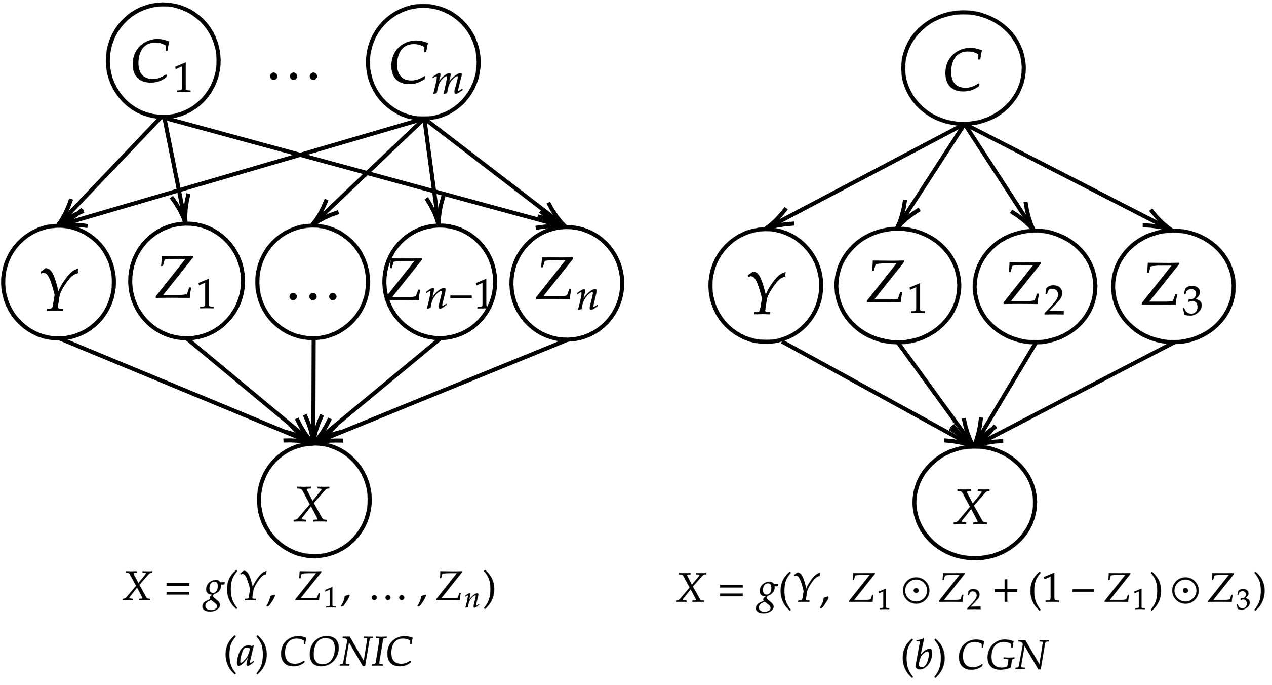
A related recent effort by (Sauer & Geiger, 2021) proposes Counterfactual Generative Networks (CGN) to address this problem using a data augmentation approach. This work assumes each image to be composed of three Independent Causal Mechanisms (ICMs) (Peters et al., 2017a) responsible for three fixed factors of variations: shape, texture, and background (as represented by , and in Figure 1(b). This work then trains a generative model that learns three ICMs for shape, texture, and background separately, and combines them in a deterministic fashion to generate observations. Once the ICMs are learned, sampling images by making interventions to these mechanisms give counterfactual data that can be used along with training data to improve classification results. However, fixing the architecture to specific number and types of mechanisms (shape, texture, background) is not generalizable, and may not directly be applicable to settings where the number of underlying generative factors is unknown. It is also computationally expensive to train different generative models for each aspect of an image such as texture, shape or background.
In this work, we begin with quantifying confounding in observational data that is generated by an underlying causal graph (more general than considered by CGN) of the form shown in Figure 1(a). We then provide a counterfactual data augmentation methodology called CONIC (COunterfactual geNeratIon under Confounding). We hypothesize that the counterfactual images generated using the proposed CONIC method provide a mechanism to marginalize the causal mechanisms responsible for spurious correlations (i.e., causal arrows from to for some ). We take a generative modeling approach and propose a neural network architecture based on conditional CycleGAN (Zhu et al., 2017) to generate counterfactual images. The proposed architecture improves CycleGAN’s ability to generate quality counterfactual images under confounded data by adding additional contrastive losses to distinguish between fixed and modified features, while learning the cross domain translations. To demonstrate the usefulness of such counterfactual images, we consider classification as a downstream task and study the performance of various models on unconfounded test set. Our key contributions include:
-
•
We formally quantify confounding in causal generative processes of the form in Fig 1(a), and study the relationship between correlation and confounding between any pair of generative factors.
-
•
We present a counterfactual data augmentation methodology to generate counterfactual instances of observed data, that can work even under highly confounded data ( confounding) and provides a mechanism to marginalize the causal mechanisms responsible for confounding.
-
•
We modify conditional CycleGAN to improve the quality of generated counterfactuals. Our method is computationally efficient and easy to implement.
-
•
Following previous work, we perform extensive experiments on well-known benchmarks – three MNIST variants and CelebA datasets – to showcase the usefulness of our proposed methodology in improving the accuracy of a downstream classifier.
2 Related Work
Counterfactual Inference: (Pearl, 2009), in his seminal text on causality, provided a three-step procedure for generation of a counterfactual data instance, given an observed instance: (i) Abduction: abduct/recover the values of exogenous noise variables; (ii) Action: perform the required intervention; and (iii) Prediction: generate the counterfactual instance. One however needs access to the underlying structural causal model (SCM) to perform the above steps for counterfactual generation. Since real-world data do not come with an underlying SCM, many recent efforts have focused on modeling the underlying causal mechanisms generating data under various assumptions. These methods then perform the required intervention on specific variables in the learned model to generate counterfactual instances that can be used for various downstream tasks such as classification, fairness, explanations etc. (Kusner et al., 2017; Joo & Kärkkäinen, 2020; Denton et al., 2019; Zmigrod et al., 2019; Pitis et al., 2020; Yoon et al., 2018; Bica et al., 2020; Pawlowski et al., 2020).
Generating Counterfactuals by Learning ICMs: In a more recent effort, assuming any real-world image is generated with three independent causal mechanisms for shape, texture, background, and a composition mechanism of the first three, (Sauer & Geiger, 2021) developed Counterfactual Generative Networks (CGN) that generate counterfactual images of a given image. CGN trains three Generative Adversarial Networks (GANs) (Goodfellow et al., 2014b) to learn shape, texture, background mechanisms and combine these three mechanisms using a composition mechanism as where is the Hadamard product. Each of these independent mechanisms is given an input of noise vector and a label specific to that independent mechanism while training. Once the independent mechanisms are trained, counterfactual images are generated by sampling a label and a noise vector corresponding to each mechanism and then feeding the input to CGN. Finally, a classifier is trained with both original and counterfactual images to achieve better test time accuracy, showing the usefulness of CGN. However, such deterministic nature of the architecture is not generalizable to the case where the number of underlying generative factors are unknown and it is computationally infeasible to train generative models for specific aspect of an image such as texture/background.
Disentanglement and Data Augmentation: The spurious correlations among generative factors have been considered in disentanglement (Funke et al., 2022; von Kügelgen et al., 2021). The general idea in these efforts is to separate the causal predictive features from non-causal/spurious predictive features to predict an outcome. Our goal is different from disentanglement, and we focus on the performance of a downstream classifier instead of separating the sources of generative factors. Traditional data augmentation methods such as rotation, scaling, corruption, etc. (Hendrycks et al., 2020; Devries & Taylor, 2017; Zhang et al., 2018; Yun et al., 2019) do not consider the causal generative process and hence they can not remove the confounding in the images via data augmentation (e.g., color and shape of an object can not be separated using simple augmentations). We hence focus on counterfactual data augmentations that is focused on marginalizing the confounding effect caused by confounders.
A similar effort to our paper is by (Goel et al., 2021) who use CycleGAN to generate counterfactual data points. However, they focus on the performance of a subgroup (a subset of data with specific properties) which is different from our goal of controlling confounding in the entire dataset. Another recent work by (Wang et al., 2022) considers spurious correlations among generative factors and uses CycleGAN to generate counterfactual images. Compared to these efforts, rather than using CycleGAN directly, we propose a CycleGAN-based architecture that is optimized for controlled generation using contrastive losses.
Applications of Counterfactuals: Augmenting the training data with appropriate counterfactual data has shown to be helpful in many applications ranging from vision to natural language tasks (Joo & Kärkkäinen, 2020; Lample et al., 2017; Kusner et al., 2017; Kaushik et al., 2019; Dash et al., 2022). (Joo & Kärkkäinen, 2020) identified existing biases in computer vision APIs deployed in the real world by Amazon, Google, IBM, and Clarifai by looking at the differences made by those APIs on counterfactual images that differ by protected/sensitive attributes (e.g., race and gender). Using locally independent causal mechanisms, (Pitis et al., 2020) augmented training data with counterfactual data points in a model-free reinforcement learning setting. Here, the idea is to use any two factual trajectories of an episode and combine the two trajectories at a particular point in time to generate the counterfactual data point, which will then be added to the replay buffer. Independently factored samples are essential to get plausible and realistic counterfactual instances.
3 Information Theoretic Measure of Confounding
Background and Problem Formulation: Let be a set of random variables denoting the generative factors of an observed data point , and be the label of the observation . Each generative factor (e.g., color) can take on a value form a discrete set of values (e.g., red, green etc.). Let the set generates real-world observations through an unknown causal mechanism . Each can be thought of as an observation generated using the causal mechanism with certain intervention on the variables in the set . Variables in may potentially be confounded by a set of confounders that denote real-world confounding such as selection bias. Let be the dataset of real-world observations along with corresponding values taken by . Causal graph in Figure 1(a) shows the general form of this setting. From a causal effect perspective, each variable in has a direct causal influence on the observation (e.g., the causal edge ) and also has non-causal influence on via the confounding variables (e.g., for some and ). These paths via the confounding variables, in which there is an incoming arrow to the variables in , are also referred to as backdoor paths (Pearl, 2001). Due to the presence of backdoor paths, we may observe spurious correlations among the variables in in the observational data .
In any downstream application where is used to train a model (e.g., classification, disentanglement etc.), it is desirable to minimize or remove the effect of confounding variable to ensure that a model is not exploiting the spurious correlations in the data to arrive at a decision. In this paper, we present a method to remove the effect of such confounding variables using counterfactual data augmentation. We start by studying the relationship between the amount of confounding and the correlation between any pair of generative factors in causal processes of the form shown in Figure 1(a).
Definition 3.1.
No Confounding (Pearl, 2009). In a causal directed acyclic graph (DAG) , where denotes the set of variables and denotes the set of directed edges denoting the direction of causal influence among the variables in , an ordered pair is unconfounded if and only if . Where denotes an intervention to the variable with the value . This definition can also be extended to disjoint sets of random variables.
Definition 3.1 provides the notion of no confounding, however, to quantify the notion of confounding between a pair of variables, we consider the following definition that relates the interventional distribution and the conditional distribution .
Definition 3.2.
(Directed Information (Raginsky, 2011; Wieczorek & Roth, 2019)). In a causal directed acyclic graph (DAG) , where denotes the set of variables and denotes the set of directed edges denoting the direction of causal influence among the variables in , the directed information from a variable to another variable is denoted by . It is defined as follows.
| (1) |
Using Definitions 3.1 and 3.2, it is easy to see that the variables and are unconfounded if and only if . Non zero directed information entails that, and hence the presence of confounding (if there is no confounder, should be equal to ). Also, it is important to note that the directed information is not symmetric (i.e., ) (Jiao et al., 2013). We use this fact in defining the measure of confounding below. Since we need to quantify the notion of confounding (as opposed to no confounding), we use directed information to quantify confounding as defined below.
Definition 3.3.
(An Information Theoretic Measure of Confounding.) In a causal directed acyclic graph (DAG) , where denotes the set of variables and denotes the set of directed edges denoting the direction of causal influence among the variables in , the amount of confounding between a pair of variables and is equal to .
Since directed information is not symmetric, we define the measure of confounding to include the directed information from one variable to the other for a given pair of variables . We now relate the quantity with the correlation between generative factors so that it is easy to quantify the amount of confounding in observational data. Before that, we present the following proposition which will be used in the proof of the subsequent proposition.
Proposition 3.1.
In causal processes of the form 1(a), the interventional distribution is same as the marginal distribution .
Proof.
In causal processes of the form 1(a), let denote the set of all confounding variables that are part of some backdoor path from to . That is for some . Then we can evaluate the quantity as
Where the first equality is because of the adjustment formula (Pearl, 2001) and the second equality is because of the fact that is a collider in causal graph 1(a) and hence conditioned on , is independent of . ∎
Proposition 3.2.
For causal generative processes of the form 1(a), the correlation between a pair of generative factors is proportional to the amount of confounding between and .
Proof.
Expanding the quantity , we get the following,
| (2) | ||||
Where is the mutual information between and . The third equality is due to Proposition 3.1. Since non-zero mutual information implies positive correlation, we see that the amount of confounding between and is directly proportional to the correlation between and . Hence, we use the correlation as a measure of confounding between generative factors in the causal processes of the form 1(a). ∎
Using the connection between the confounding and correlation in causal graph 1(a), our objective is to generate counterfactual data such that the resultant dataset after augmentation looks similar to the data obtained from a causal process where there is no confounding between generative factors (i.e., no paths of the from ). Equivalently, our counterfactual data generation algorithm removes the spurious correlations between generative factors by marginalizing the causal arrows for some . To understand how counterfactual instances break the correlations, consider the following definition.
Definition 3.4.
(Counterfactual (Pearl, 2009)). Given an observed instance whose generative factors take on the values , the counterfactual instance of (generated using the 3-step counterfactual inference procedure) differed from w.r.t. the generative factor , is an instance whose generative factors take on the values . Here ’s value is changed from to through an external intervention .
If we observe spurious correlation between two generative factors when they take on the values and respectively, generating counterfactual instances w.r.t. with the intervention and adding the counterfactual instances to original data breaks the correlation between . With this idea, we now present our algorithm to generate counterfactual images in a systematic manner remove confounding from observational data.
4 CONIC: Methodology
Our goal is to remove the effect of confounding in the observational data on a downstream task such as classification. To this end, we propose a way to systematically generate counterfactual data that can marginalize the effect of any confounding edge in Fig. 1 (a) as explained below.
Removing The Confounding Effect of : In the causal graphs of the form 1(a), for paths of the form , we call the edges and as confounding edges since together, their existence is the reason for confounding in the data. Also, let is one pair of attribute values taken by the variable pair under extreme confounding (e.g., in the training set of colored MNIST dataset, correlation coefficient of between color and digit is observed such that whenever color is red, digit is etc.). To remove the effect of the confounding edge w.r.t. the another confounding edge (recall that confounding between is present if and only if there exists a pair of causal arrows and for some ; due to this reason we consider the confounding effect of the confounding edge w.r.t. another confounding edge ), we consider two subsets of the observational data which are constructed as follows. consists of the set of instances for which and , consists of the set of instances for which and . The size of is usually much smaller than the size of because of high correlation between and (e.g., there are more red ’s than non-red ’s).
Now, we learn a mapping from the set to the set that changes the attribute while fixing the value of at . That is, for any given instance , for which , maps to a different instance in which the value of the generative factor is changed to (e.g., takes red as input and returns red as output). This mapping can be thought of as a function performing the 3-step counterfactual inference: learning the underlying generative factors, performing the intervention and then generating the counterfactual instance . Now, given an instance for which and , using , we can generate counterfactual instance in which and . These counterfactual instances, when augmented with the original observed dataset , removes the effect of the confounding edge w.r.t. the edge . That is, the counterfactual instances, when augmented with original data, breaks the correlation between and . This process can now be repeated systematically for each confounding edge to generate counterfactual instances that remove the spurious correlations. Such augmented data points which differ from original data points w.r.t. only one feature (e.g., if original image is a male with blond hair color, augmented image is same male with black hair color) are referred as coupled sets by (Goel et al., 2021), images generated by causal essential transformations by (Wang et al., 2022). The overall procedure to generate counterfactual instances is summarized in Algorithm 1.
Earlier works use CycleGAN to generate counterfactual images that differ from original image by a single attribute/feature (Wang et al., 2022; Goel et al., 2021). Given two domains/sets of images that differ w.r.t. only one generative factor , a CycleGAN can learn to translate between the two domains by changing the attribute value of . In this case, one can think of CycleGAN as a function performing the required intervention and generating counterfactual instance without modeling the underlying causal process. Concretely, CycleGAN is an architecture used to perform unsupervised domain translation using unpaired images. In a CycleGAN, a generator first transforms a given image from a domain/set into so that appears to come from another domain/set such that certain features from input are preserved in the output . A discriminator then classifies whether the translated image is original (i.e., sampled from ) or fake (i.e., generated by ). A second generator transforms the image back to original image to ensure that is using the contents of to generate . The same procedure is repeated to translate images from domain into domain . The loss function of CycleGAN can be written as follows.
| (3) |
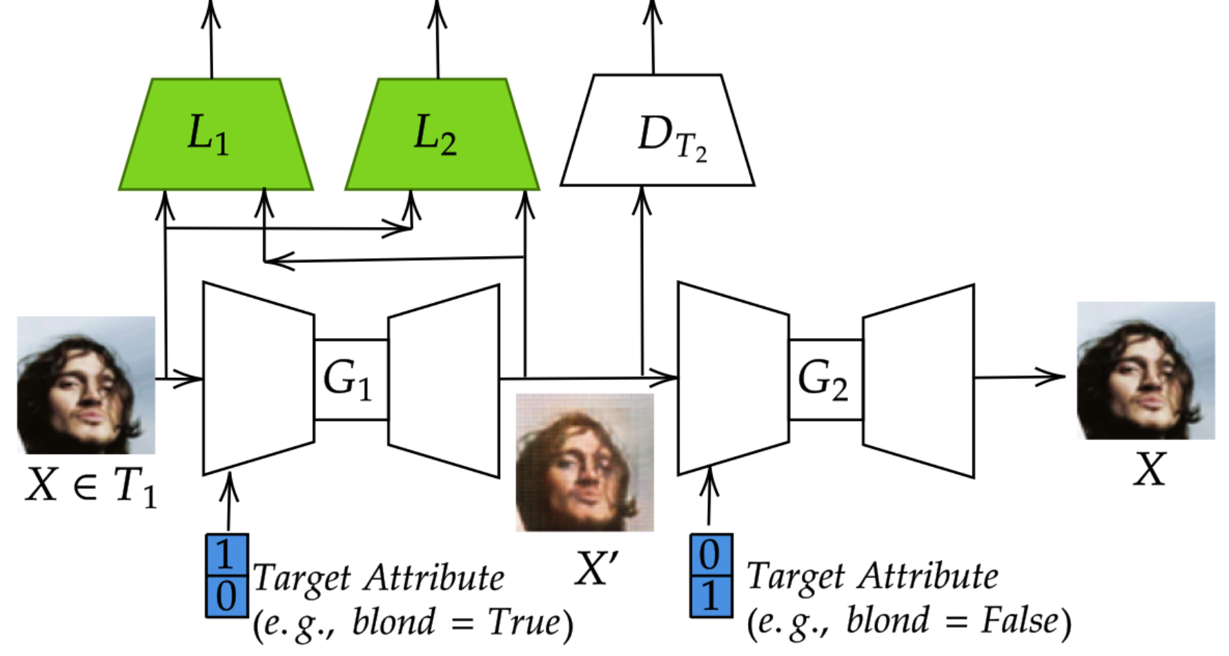
Where is simple Generative Adversarial Network (GAN) (Goodfellow et al., 2014a) loss and is cycle consistency loss measuring how well the output of is matching with the original input . For example, can ensure that . In this work, to learn the mapping function , we use conditional variant of CycleGAN to leverage the supervision in terms of attribute values. For each generator, along with input, we also feed a desired target attribute as shown in the Figure 2.
To improve the quality of counterfactual images generated by conditional CycleGAN under extreme confounding, we propose a modification to conditional CycleGAN as detailed below. As discussed earlier, , the output of , can be thought of as a counterfactual image of . When changing the feature of , we keep the feature fixed. That is, the representation for in both and should be different and the representation for in both and should be same. To ensure this, as shown in Figure 2, along with two generators and a discriminator that are part of conditional CycleGAN, we add two pre-trained discriminators (shown in green color in Fig. 2). takes two images as input and returns high penalty if the representation of is similar in and small penalty otherwise. takes two images as input and returns high penalty if the representation of is different and small penalty otherwise. Thus, our overall objective to generate good quality counterfactual images is to train the modified conditional CycleGAN by minimizing the following objective.
| (4) | ||||
Where is a hyperparameter and is the contrastive loss (Hadsell et al., 2006). For a pair of images , defined as follows.
| (5) |
Where if belong to same class (or have same attribute values), if belong to different classes (or have different attribute values). is the distance between the representations of (e.g., Euclidean distance). is the margin of error allowed between two representations of the images of different classes. and are pre-trained models and the parameters of and are fixed. That is, the loss values returned by are only used to update the trainable parameters of conditional CycleGAN.
A Downstream Task - Image Classification: To measure the goodness of counterfactual generation under confounding using Algorithm 1, we consider the classification task on the unconfounded test set as a downstream task. Let be the dataset consisting of original data points from and corresponding counterfactual data points. Usual empirical risk minimizer minimizes the following loss over .
| (6) |
Where is cross entropy loss. Using , we minimize the following loss :
| (7) |
To further improve the performance of a classifier using , for each pair of images we minimize the contrastive loss on the logits in the final layer. Now, the final objective to optimize for classification task is to minimize the following loss.
| (8) |
Where is a regularization hyperparameter.
5 Experiments and Results
In this section, we present the experimental results on both synthetic (MNIST variants) and real world (CelebA) datasets. Having access to the ground truth generative factors (i.e., ) of images,we artificially create confounding in the training data and we leave test data to be unconfounded (i.e., no correlation among generative factors). We compare CONIC with various baselines including traditional Empirical Risk Minimizer (ERM), Conditional GAN (CGAN) (Goodfellow et al., 2014a), Conditional VAE (CVAE) (Kingma & Welling, 2013), Conditional--VAE (C--VAE) (Higgins et al., 2017), AugMix (Hendrycks et al., 2020), CutMix (Yun et al., 2019), Invariant Risk Minimization (IRM) (Arjovsky et al., 2019), and Counterfactual Generative Networks (CGN) (Sauer & Geiger, 2021). To check the goodness of each of these methods, we check how well the performance of the downstream classifier on the test set is improved using the augmented images.
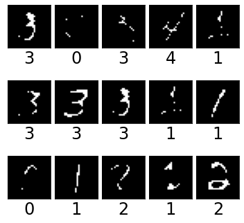
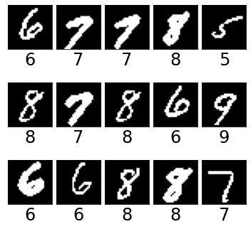
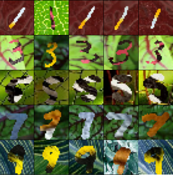
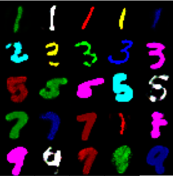
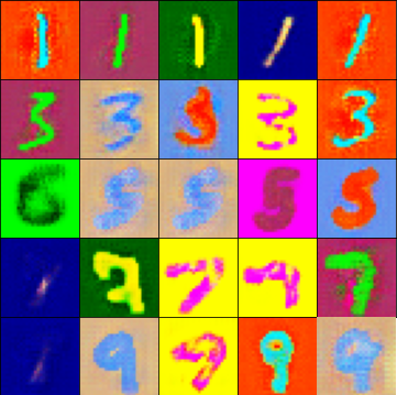
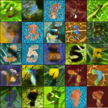
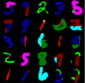
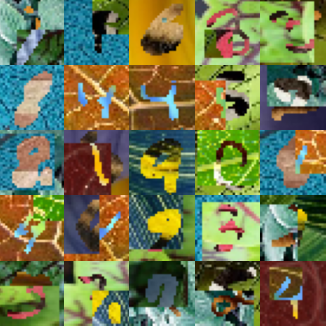
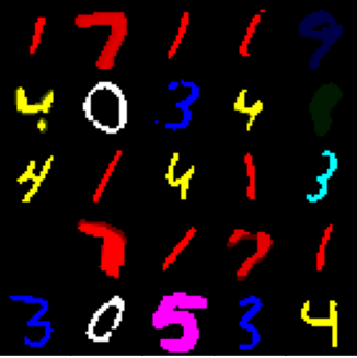
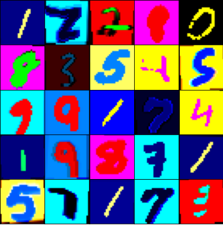
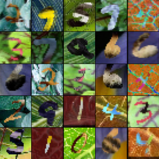
MNIST Variants: We construct the following three synthetic datasets based on MNIST dataset (Lecun et al., 1998) and its colored, texture, and morpho (where the digit thickness is controlled; Fig. 3) variants (Arjovsky et al., 2019; Castro et al., 2019; Sauer & Geiger, 2021): (i) colored morpho MNIST (CM-MNIST), (ii) double colored morpho MNIST (DCM-MNIST), and (iii) wildlife morpho MNIST (WLM-MNIST). We consider extreme confounding among generative factors as explained below.
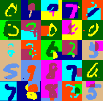
For the experimental results shown in Table 1, in the training set of CM-MNIST dataset, the correlation coefficient between digit label and digit color is and the digits from to are thin and digits from to are thick (see Figure 3). That is, if the digit is in [0,1,2,3,4] else . In the training set of DCM-MNIST dataset, digit label, digit color, and background color jointly take a fixed set of values 95% of the time. That is, and the digits from to are thin and digits from to are thick. In the training set of WLM-MNIST dataset digit shape, digit texture, and background texture jointly take a fixed set of attribute values 95% of the time and the digits from to are thin and digits from to are thick.
| Model | CM-MNIST | DCM-MNIST | WLM-MNIST | CelebA |
|---|---|---|---|---|
| ERM | 46.41 0.81% | 43.31 2.30% | 28.28 0.70% | 70.64 6.93% |
| CGAN | 41.86 1.79% | 30.66 3.86% | 17.50 0.85% | 70.99 2.35% |
| CVAE | 49.58 1.50% | 41.99 1.10% | 34.19 1.58% | 71.50 1.82% |
| C--VAE | 51.22 1.00% | 51.58 2.36% | 33.90 1.87% | 74.29 0.65% |
| AugMix | 47.36 0.01% | 44.85 0.02% | 26.30 1.30% | 71.93 4.64% |
| CutMix | 20.44 1.22% | 23.10 2.98% | 12.08 1.59% | 73.66 0.76% |
| IRM | 55.25 0.89% | 49.71 0.71% | 50.26 0.48% | 72.30 2.71% |
| CGN | 42.15 3.89% | 47.50 2.18% | 43.84 0.25% | 69.25 0.29% |
| CONIC | 65.57 0.34% | 92.41 0.26% | 77.72 1.00% | 79.56 1.28% |
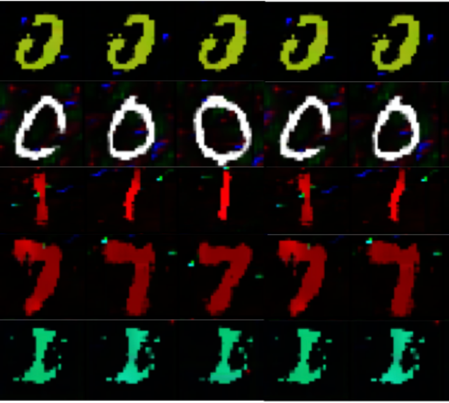
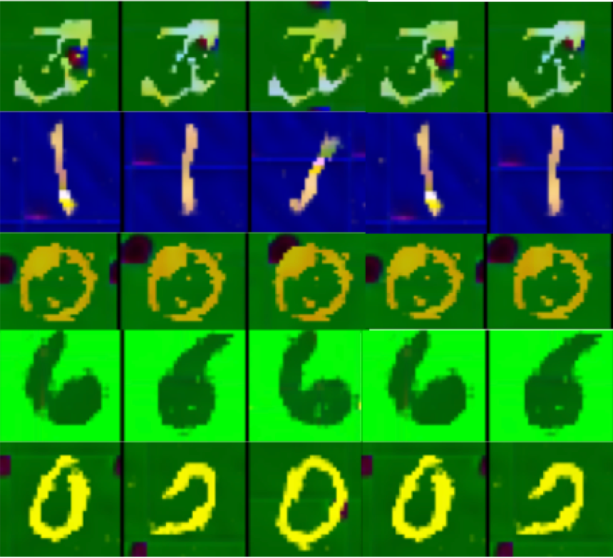
In all of these MNIST variants, test set images are unconfounded (e.g., in the test set of DCM-MNIST, any digit can be thin or think, can be in any background color, can be in any foreground color). In these experiments, under extreme confounding, our goal is to generate counterfactual images that break the confounding among generative factors. We evaluate models on this grounds by training a classifier using the augmented data and testing it on the unconfounded test data. Table 1 shows the results in which CONIC outperforms all the baselines. See Appendix for comparison of augmented images by various baselines. Coninc uses only , , counterfactual images in CM-MNIST, DCM-MNIST, and WLM-MNIST experiments as augmented images respectively to get improved performance. The regularization hyperparameter in Equation 8 set to for all MNIST experiments.
CelebA: Unlike MNIST variants, CelebA (Liu et al., 2015) dataset implicitly contains confounding (e.g., the percentage of males with blond hair is different from the percentage of females with blond hair, in addition to the difference in the total number of males and females in the dataset). In this experiment, we consider the performance of a classifier trained on the augmented data that predicts hair color given an image. Our test set is the set of males with blond hair.
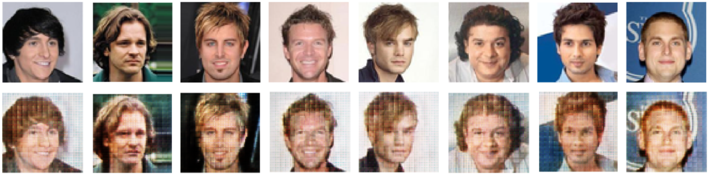
We train models on the train set and test the performance on the set of males with blond hair. Since the number of males with blond hair is very low in the dataset (approximately 4% of males have blond hair), we show that the augmenting the train set with only 10000 images of males with blond hair improves the performance over baselines (see Table 1) whereas other baselines require more than 50000 augmented images to get minor improvement over ERM. Given a male image with non-blond hair, CONIC generates the counterfactual image with blond hair without changing the male attribute (see Figure 4 for sample counterfactual images). We also note that the deterministic models such as CGN fail when they are applied to a different task where the number and type of generative factors are not fixed and are difficult to separate (e.g., CelebA). CGN results in table 1 are obtained with only 1000 counterfactual images as augmented data points. When we increase the number of counterfactual instances, performance of CGN reduces further.
Time Complexity Analysis: Apart from its simple methodology, CONIC brings
| Dataset | CONIC | CGN |
|---|---|---|
| CM-MNIST | 2.76 0.19 | 103 1.50 |
| DCM-MNIST | 2.22 0.01 | 103 2.04 |
| WLM-MNIST | 1.22 0.01 | 111 2.50 |
additional advantages in terms of computing time required to train the model that generates counterfactual images. As shown in Table 2, the time required to run our method to generate counterfactual images w.r.t. a generative factor is significantly less than CGN that learns deterministic causal mechanisms as discussed in Section 2. Even though we used CycleGAN in this work, for the cases where the number of generative factors are more, StarGAN (Choi et al., 2018) can be used to minimize the time required to learn the mappings from one domain to another domain (Wang et al., 2022; Goel et al., 2021).
6 Conclusions
We studied the adverse effects of confounding in observational data on the performance of a classifier. We showed the relationship between confounding and correlation in the causal processes considered, and we proposed a methodology to remove the correlation between the target variable and generative factors that works even when the dataset is highly confounded. Specifically, we proposed a counterfactual data augmentation method that systematically removes the confounding effect rather than addressing the confounding problem through random augmentations. Using the generated counterfactuals leads to substantial increase in a downstream classifier’s accuracy. That said, we observed that the counterfactual quality can still be improved, which will be interesting future work.
References
- dif (2022) Diffusion causal models for counterfactual estimation, 2022.
- Arjovsky et al. (2019) Martin Arjovsky, Léon Bottou, Ishaan Gulrajani, and David Lopez-Paz. Invariant risk minimization, 2019.
- Atzmon et al. (2020) Yuval Atzmon, Felix Kreuk, Uri Shalit, and Gal Chechik. A causal view of compositional zero-shot recognition. In NeurIPS, 2020.
- Bica et al. (2020) Ioana Bica, James Jordon, and Mihaela van der Schaar. Estimating the effects of continuous-valued interventions using generative adversarial networks. In H. Larochelle, M. Ranzato, R. Hadsell, M. F. Balcan, and H. Lin (eds.), NeurIPS, volume 33, pp. 16434–16445. Curran Associates, Inc., 2020. URL https://proceedings.neurips.cc/paper/2020/file/bea5955b308361a1b07bc55042e25e54-Paper.pdf.
- Castro et al. (2019) Daniel C. Castro, Jeremy Tan, Bernhard Kainz, Ender Konukoglu, and Ben Glocker. Morpho-MNIST: Quantitative assessment and diagnostics for representation learning. JMLR, 20(178), 2019.
- Choi et al. (2018) Yunjey Choi, Minje Choi, Munyoung Kim, Jung-Woo Ha, Sunghun Kim, and Jaegul Choo. Stargan: Unified generative adversarial networks for multi-domain image-to-image translation. In CVPR, 2018.
- Dash et al. (2022) Saloni Dash, Vineeth N Balasubramanian, and Amit Sharma. Evaluating and mitigating bias in image classifiers: A causal perspective using counterfactuals. In WACV, 2022.
- Denton et al. (2019) Emily Denton, Ben Hutchinson, Margaret Mitchell, and Timnit Gebru. Detecting bias with generative counterfactual face attribute augmentation, 2019.
- Devries & Taylor (2017) Terrance Devries and Graham W. Taylor. Improved regularization of convolutional neural networks with cutout. ArXiv, abs/1708.04552, 2017.
- Dinga et al. (2020) Richard Dinga, Lianne Schmaal, Brenda W.J.H. Penninx, Dick J. Veltman, and Andre F. Marquand. Controlling for effects of confounding variables on machine learning predictions. bioRxiv, 2020.
- Funke et al. (2022) Christina M Funke, Paul Vicol, Kuan-Chieh Wang, Matthias Kuemmerer, Richard Zemel, and Matthias Bethge. Disentanglement and generalization under correlation shifts. In ICLR2022 Workshop on the Elements of Reasoning: Objects, Structure and Causality, 2022. URL https://openreview.net/forum?id=H8QVUSuIqgq.
- Goel et al. (2021) Karan Goel, Albert Gu, Yixuan Li, and Christopher Re. Model patching: Closing the subgroup performance gap with data augmentation. In ICLR, 2021.
- Goodfellow et al. (2014a) Ian J. Goodfellow, Jean Pouget-Abadie, Mehdi Mirza, Bing Xu, David Warde-Farley, Sherjil Ozair, Aaron Courville, and Yoshua Bengio. Generative adversarial networks, 2014a.
- Goodfellow et al. (2014b) Ian J. Goodfellow, Jean Pouget-Abadie, Mehdi Mirza, Bing Xu, David Warde-Farley, Sherjil Ozair, Aaron C. Courville, and Yoshua Bengio. Generative adversarial nets. In NIPS, pp. 2672–2680, 2014b. URL http://papers.nips.cc/paper/5423-generative-adversarial-nets.
- Hadsell et al. (2006) R. Hadsell, S. Chopra, and Y. LeCun. Dimensionality reduction by learning an invariant mapping. In CVPR, 2006.
- Hendrycks et al. (2020) Dan Hendrycks, Norman Mu, Ekin Dogus Cubuk, Barret Zoph, Justin Gilmer, and Balaji Lakshminarayanan. Augmix: A simple method to improve robustness and uncertainty under data shift. In ICLR, 2020. URL https://openreview.net/forum?id=S1gmrxHFvB.
- Higgins et al. (2017) Irina Higgins, Loic Matthey, Arka Pal, Christopher Burgess, Xavier Glorot, Matthew Botvinick, Shakir Mohamed, and Alexander Lerchner. beta-VAE: Learning basic visual concepts with a constrained variational framework. In International Conference on Learning Representations, 2017. URL https://openreview.net/forum?id=Sy2fzU9gl.
- Hu & Li (2021) Zhiting Hu and Li Erran Li. A causal lens for controllable text generation. In A. Beygelzimer, Y. Dauphin, P. Liang, and J. Wortman Vaughan (eds.), Advances in Neural Information Processing Systems, 2021. URL https://openreview.net/forum?id=kAm9By0R5ME.
- Idrissi et al. (2022) Badr Youbi Idrissi, Martin Arjovsky, Mohammad Pezeshki, and David Lopez-Paz. Simple data balancing achieves competitive worst-group-accuracy. In Proceedings of the First Conference on Causal Learning and Reasoning, volume 177 of Proceedings of Machine Learning Research, 2022.
- Jiao et al. (2013) Jiantao Jiao, Haim H Permuter, Lei Zhao, Young-Han Kim, and Tsachy Weissman. Universal estimation of directed information. IEEE Transactions on Information Theory, 59(10):6220–6242, 2013.
- Joo & Kärkkäinen (2020) Jungseock Joo and Kimmo Kärkkäinen. Gender slopes: Counterfactual fairness for computer vision models by attribute manipulation. In Proceedings of the 2nd International Workshop on Fairness, Accountability, Transparency and Ethics in Multimedia, FATE/MM ’20, pp. 1–5, New York, NY, USA, 2020. Association for Computing Machinery. ISBN 9781450381482. doi: 10.1145/3422841.3423533. URL https://doi.org/10.1145/3422841.3423533.
- Joshi & He (2022) Nitish Joshi and He He. An investigation of the (in)effectiveness of counterfactually augmented data. In Proceedings of the 60th Annual Meeting of the Association for Computational Linguistics (Volume 1: Long Papers), pp. 3668–3681, Dublin, Ireland, May 2022. Association for Computational Linguistics.
- Kaushik et al. (2019) Divyansh Kaushik, Eduard Hovy, and Zachary C Lipton. Learning the difference that makes a difference with counterfactually-augmented data. arXiv preprint arXiv:1909.12434, 2019.
- Kilbertus et al. (2020) Niki Kilbertus, Philip J Ball, Matt J Kusner, Adrian Weller, and Ricardo Silva. The sensitivity of counterfactual fairness to unmeasured confounding. In UAI, 2020.
- Kingma & Welling (2013) Diederik P Kingma and Max Welling. Auto-encoding variational bayes, 2013.
- Kusner et al. (2017) Matt J Kusner, Joshua Loftus, Chris Russell, and Ricardo Silva. Counterfactual fairness. In I. Guyon, U. V. Luxburg, S. Bengio, H. Wallach, R. Fergus, S. Vishwanathan, and R. Garnett (eds.), NeurIPS, volume 30. Curran Associates, Inc., 2017. URL https://proceedings.neurips.cc/paper/2017/file/a486cd07e4ac3d270571622f4f316ec5-Paper.pdf.
- Lample et al. (2017) Guillaume Lample, Neil Zeghidour, Nicolas Usunier, Antoine Bordes, Ludovic DENOYER, and Marc' Aurelio Ranzato. Fader networks:manipulating images by sliding attributes. In NeurIPS, 2017.
- Lecun et al. (1998) Y. Lecun, L. Bottou, Y. Bengio, and P. Haffner. Gradient-based learning applied to document recognition. Proceedings of the IEEE, 86(11):2278–2324, 1998. doi: 10.1109/5.726791.
- Liu et al. (2015) Ziwei Liu, Ping Luo, Xiaogang Wang, and Xiaoou Tang. Deep learning face attributes in the wild. In ICCV, 2015.
- Meinshausen & Bühlmann (2015) Nicolai Meinshausen and Peter Bühlmann. Maximin effects in inhomogeneous large-scale data. The Annals of Statistics, 43(4):1801 – 1830, 2015.
- Pawlowski et al. (2020) Nick Pawlowski, Daniel Coelho de Castro, and Ben Glocker. Deep structural causal models for tractable counterfactual inference. In H. Larochelle, M. Ranzato, R. Hadsell, M. F. Balcan, and H. Lin (eds.), NeurIPS, volume 33, pp. 857–869. Curran Associates, Inc., 2020. URL https://proceedings.neurips.cc/paper/2020/file/0987b8b338d6c90bbedd8631bc499221-Paper.pdf.
- Pearl (2001) Judea Pearl. Direct and indirect effects. In UAI, pp. 411–420, 2001.
- Pearl (2009) Judea Pearl. Causality. Cambridge university press, 2009.
- Peters et al. (2017a) J. Peters, D. Janzing, and B. Schölkopf. Elements of Causal Inference: Foundations and Learning Algorithms. MIT Press, Cambridge, MA, USA, 2017a.
- Peters et al. (2017b) J. Peters, D. Janzing, and B. Scholkopf. Elements of Causal Inference: Foundations and Learning Algorithms. Adaptive Computation and Machine Learning series. MIT Press, 2017b.
- Pitis et al. (2020) Silviu Pitis, Elliot Creager, and Animesh Garg. Counterfactual data augmentation using locally factored dynamics. In H. Larochelle, M. Ranzato, R. Hadsell, M. F. Balcan, and H. Lin (eds.), NeurIPS, volume 33, pp. 3976–3990. Curran Associates, Inc., 2020. URL https://proceedings.neurips.cc/paper/2020/file/294e09f267683c7ddc6cc5134a7e68a8-Paper.pdf.
- Raginsky (2011) Maxim Raginsky. Directed information and pearl’s causal calculus. In 2011 49th Annual Allerton Conference on Communication, Control, and Computing (Allerton), pp. 958–965, 2011. doi: 10.1109/Allerton.2011.6120270.
- Reddy et al. (2022) Abbavaram Gowtham Reddy, Benin L Godfrey, and Vineeth N Balasubramanian. On causally disentangled representations. In AAAI, 2022.
- Ronneberger et al. (2015) O. Ronneberger, P.Fischer, and T. Brox. U-net: Convolutional networks for biomedical image segmentation. In Medical Image Computing and Computer-Assisted Intervention (MICCAI), volume 9351 of LNCS, pp. 234–241. Springer, 2015.
- Rothenhäusler et al. (2021) Dominik Rothenhäusler, Nicolai Meinshausen, Peter Bühlmann, Jonas Peters, et al. Anchor regression: Heterogeneous data meet causality. Journal of the Royal Statistical Society Series B, 83(2):215–246, 2021.
- Sauer & Geiger (2021) Axel Sauer and Andreas Geiger. Counterfactual generative networks. In ICLR, 2021.
- Schölkopf et al. (2021) Bernhard Schölkopf, Francesco Locatello, Stefan Bauer, Nan Rosemary Ke, Nal Kalchbrenner, Anirudh Goyal, and Yoshua Bengio. Towards causal representation learning. CoRR, abs/2102.11107, 2021. URL https://arxiv.org/abs/2102.11107.
- Suter et al. (2019) Raphael Suter, Djordje Miladinovic, Bernhard Schölkopf, and Stefan Bauer. Robustly disentangled causal mechanisms: Validating deep representations for interventional robustness. In ICML, 2019.
- Träuble et al. (2021) Frederik Träuble, Elliot Creager, Niki Kilbertus, Francesco Locatello, Andrea Dittadi, Anirudh Goyal, Bernhard Schölkopf, and Stefan Bauer. On disentangled representations learned from correlated data. In ICML, 2021.
- von Kügelgen et al. (2021) Julius von Kügelgen, Yash Sharma, Luigi Gresele, Wieland Brendel, Bernhard Schölkopf, Michel Besserve, and Francesco Locatello. Self-supervised learning with data augmentations provably isolates content from style. In NeurIPS, 2021.
- Von Kügelgen et al. (2021) Julius Von Kügelgen, Yash Sharma, Luigi Gresele, Wieland Brendel, Bernhard Schölkopf, Michel Besserve, and Francesco Locatello. Self-supervised learning with data augmentations provably isolates content from style. Advances in neural information processing systems, 34:16451–16467, 2021.
- Wang et al. (2022) Ruoyu Wang, Mingyang Yi, Zhitang Chen, and Shengyu Zhu. Out-of-distribution generalization with causal invariant transformations. In CVPR, 2022.
- Wieczorek & Roth (2019) Aleksander Wieczorek and Volker Roth. Information theoretic causal effect quantification. Entropy, 21(10), 2019.
- Yoon et al. (2018) Jinsung Yoon, James Jordon, and Mihaela van der Schaar. GANITE: estimation of individualized treatment effects using generative adversarial nets. In 6th ICLR, ICLR 2018, Vancouver, BC, Canada, April 30 - May 3, 2018, Conference Track Proceedings. OpenReview.net, 2018. URL https://openreview.net/forum?id=ByKWUeWA-.
- Yue et al. (2021) Zhongqi Yue, Tan Wang, Qianru Sun, Xian-Sheng Hua, and Hanwang Zhang. Counterfactual zero-shot and open-set visual recognition. In CVPR, 2021.
- Yun et al. (2019) Sangdoo Yun, Dongyoon Han, Sanghyuk Chun, Seong Joon Oh, Youngjoon Yoo, and Junsuk Choe. Cutmix: Regularization strategy to train strong classifiers with localizable features. In ICCV, pp. 6022–6031, 2019. doi: 10.1109/ICCV.2019.00612.
- Zhang et al. (2018) Hongyi Zhang, Moustapha Cisse, Yann N. Dauphin, and David Lopez-Paz. mixup: Beyond empirical risk minimization. In ICLR, 2018. URL https://openreview.net/forum?id=r1Ddp1-Rb.
- Zhao et al. (2020) Qingyu Zhao, Ehsan Adeli, and Kilian M Pohl. Training confounder-free deep learning models for medical applications. Nature communications, 11(1):1–9, 2020.
- Zhu et al. (2017) Jun-Yan Zhu, Taesung Park, Phillip Isola, and Alexei A. Efros. Unpaired image-to-image translation using cycle-consistent adversarial networks. In ICCV, 2017.
- Zmigrod et al. (2019) Ran Zmigrod, Sabrina J. Mielke, Hanna Wallach, and Ryan Cotterell. Counterfactual data augmentation for mitigating gender stereotypes in languages with rich morphology, 2019.
Appendix
In this appendix, we include the following additional information, which we could not fit in the main paper due to space constraints:
-
•
Additional implementation details
-
•
More details on related work
-
•
Empirical evidence on the relationship between confounding and correlation
-
•
Ablation studies
-
•
Counterfactual images of MNIST variants for various methods
Appendix A Additional Implementation Details
The generators used in CycleGAN are U-Networks Ronneberger et al. (2015) made of a 4-layer encoder and a 4-layer decoder. The discriminators are 4-layer encoders that output the probability of an image being a particular class. Since all the contrastive loss terms in Equation 4 work together towards removing the confounding effect of a confounding edge (unlike loss functions where each term has a different purpose). Hence, we use a common weighting term in Equation 4. For all the experiments, batch size of 256 is used to train classifier (Equation 8). In all of the architectures, leaky-relu activation is used as an activation and sigmoid activation is used in the final layer to get probabilities. Adam optimizer is used in all the experiments.
Appendix B More on Related Work
In this section, we continue with the related work presented in the Section 2 of the main paper. Joshi & He (2022) discusses a potential issue for a counterfactual data augmentation method, viz.: if counterfactual data augmentation does not consider/augment counterfactuals w.r.t. all robust features that are spuriously correlated with non-robust features, then the performance of a model may drop in unseen distributions. To contrast this with our work, since we are able to quantify the confounding and hence correlation between any pair of generative factors, CONIC can generate all possible counterfactuals, which may in fact help in generate counterfactual images w.r.t. all robust/causal features. Hence, models trained on the counterfactual images generated using CONIC are more robust.
Idrissi et al. (2022) is similar to our work in performing data augmentation (for e.g., results on CelebA) with a difference that our method can be extended to the performance on the entire test set instead of on the worst group (e.g., MNIST results). Also, Hu & Li (2021) is similar in a sense to our work, but aims at controllable generation and counterfactual generation in the natural language setting. dif (2022) also generates counterfactual images but it assumes the availability of the data generation process and does not explicitly tackle confounding. Our work only assumes access to the attribute information but not the data generating process.
Appendix C Relationship between correlation and confounding
Table 3 shows the empirical evidence that confounding is directly proportional to correlation between generative factors in CM-MNIST dataset.
| Correlation Coefficient (color, digit) | Confounding (color, digit) (Defn 3) |
| 0.10 | 0.072 |
| 0.20 | 0.249 |
| 0.50 | 1.244 |
| 0.90 | 3.585 |
| 0.95 | 4.041 |
Appendix D Ablation Studies
In this section, we present the results on some ablation studies to understand the usefulness of the proposed regularizers. Without the additional regularizers in Eqn 4, the accuracy on the downstream classifier on CelebA is . However, using the additional regularizer, the accuracy improves upto . The additional contrastive loss in Eqn 8 brings a slight improvement over Eqn 7. In CelebA experiments, while accuracy obtained when using Eqn 7 is around but using Eqn 8, the accuracy improved to .
Also, to understand the performance of ERM model using only the 5% unconfounded data, we experimented on MNIST variants and observed that the accuracy on CM-MNIST, DCM-MNIST, and WLM-MNIST are , , , respectively. These results are worse than ERM model trained on entire training dataset (Table 1). We believe that the reason for these poor results by ERM model is due to the presence of multiple confounders. In MNIST variants, along with the confounding between color and digit, there is another feature called thickness that is challenging to learn, especially when the digits are thin (Figure 3 left). When we take only 5% unconfounded data, the train set size is very small, with many thin digits, making it difficult for ERM to learn the features.
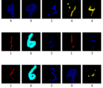
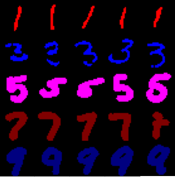
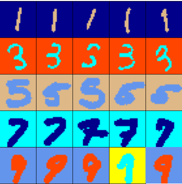
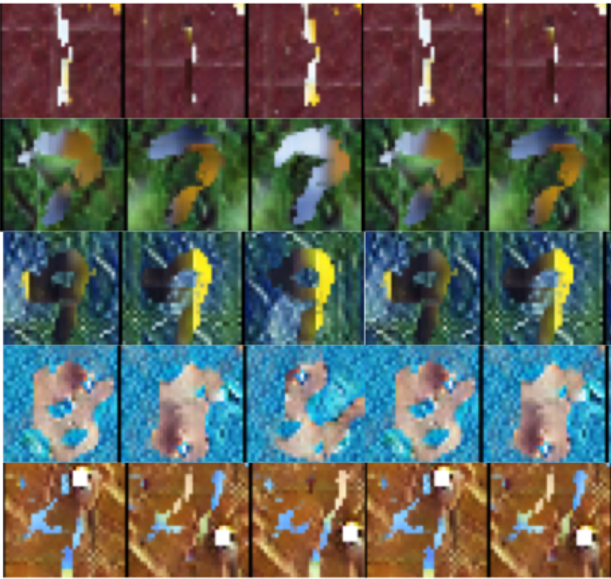
Appendix E Counterfactual Images by Various Methods
Figure 5 and 6 shows the counterfactual images generated by various methods on MNIST variants.
 CM-MNIST Samples
 DCM-MNIST Samples
 WLM-MNIST Samples
 CM-MNIST CONIC
 DCM-MNIST CONIC
 WLM-MNIST CONIC
 CM-MNIST CUTMix
 DCM-MNIST CUTMix
 WLM-MNIST CUTMix
 CM-MNIST AUGMix
 DCM-MNIST AUGMix
 WLM-MNIST AUGMix
 CM-MNIST CGN
 DCM-MNIST CGN
 WLM-MNIST CGN