Coupled Layer-wise Graph Convolution for Transportation Demand Prediction
Abstract
Graph Convolutional Network (GCN) has been widely applied in transportation demand prediction due to its excellent ability to capture non-Euclidean spatial dependence among station-level or regional transportation demands. However, in most of the existing research, the graph convolution was implemented on a heuristically generated adjacency matrix, which could neither reflect the real spatial relationships of stations accurately, nor capture the multi-level spatial dependence of demands adaptively. To cope with the above problems, this paper provides a novel graph convolutional network for transportation demand prediction. Firstly, a novel graph convolution architecture is proposed, which has different adjacency matrices in different layers and all the adjacency matrices are self-learned during the training process. Secondly, a layer-wise coupling mechanism is provided, which associates the upper-level adjacency matrix with the lower-level one. It also reduces the scale of parameters in our model. Lastly, a unitary network is constructed to give the final prediction result by integrating the hidden spatial states with gated recurrent unit, which could capture the multi-level spatial dependence and temporal dynamics simultaneously. Experiments have been conducted on two real-world datasets, NYC Citi Bike and NYC Taxi, and the results demonstrate the superiority of our model over the state-of-the-art ones.
Introduction
Recently Intelligent Transportation System (ITS) has become a hot research spot, which is mainly contributed by the two following factors: 1) the rapid development of urban transportation, and 2) the wide application of big data technology in transportation information system. Even though, there are still several important problems that remain to be dug into, such as traffic environment monitoring, travel route recommendation, in which transportation demand prediction is the most essential and crucial issue. By obtaining the precise number of the demand in each region in advance, the transport resource can be pre-allocated and re-balanced to maximize the transportation capacity, and residents will be provided with a better service in daily travel.
Due to the importance of transportation demand prediction, many efforts have been made in this field in the past few years. The development of mainstream could be divided into three stages: 1) The researches in the early time employed the empirical statistical analysis which mainly focus on forecasting the demand in a specific region instead of the whole city (Moreira-Matias et al. 2013; Liu et al. 2016), and the incapability of capturing spatial and temporal correlation simultaneously leads to relatively low prediction accuracy. 2) Recently, deep learning grows up quickly and gives us a new solution of modeling spatio-temporal correlations. By treating the entire city as an image and partitioning it into several grids, researchers employ Convolutional Neural Network (CNN) to extract spatial correlations (Zhang, Zheng, and Qi 2017) and Recurrent Neural Network (RNN) to extract temporal correlations (Yao et al. 2018), which makes a huge progress on the formalization. However, aggregating with neighbors in space makes CNN-based methods insensitive to long-distance transition patterns and only fit for Euclidean spatial relationship. 3) Graph convolutional network, a generalization of CNN, is fit to deal with non-Euclidean data naturally. Due to topological structure of road networks, it has been successfully and widely applied in transportation field. Li et al. (2017) first extracted spatial dependency with diffusion graph convolution network in traffic forecasting problem. Yu, Yin, and Zhu (2017) combined GCN with casual convolutional network, and stacked the blocks to capture spatio-temporal dependence simultaneously.
Though GCN has demonstrated its effectiveness in transportation prediction problem, there are still four important issues which have not been discussed elaborately: 1) The adjacency matrix which determines the aggregation manner in the graph convolutional network is mostly fixed and generated by heuristic methods according to spatial distance or network connectivity, which cannot capture the genuine spatial dependence. 2) Existing methods ignore the hierarchical dependence of transportation demand prediction. For example, a sudden rainstorm causes the global reduction of sharing bike usage, but a congestion led by traffic accident can only make a local impact. 3) Mainly following the perspective of graph signal processing, current graph convolution approaches tend to smooth nodes’ input signals. In this situation, it is difficult for stacked graph convolution layers with only one adjacency matrix to obtain multi-level representations of transportation demand efficiently. 4) The representations in different layers contributing to the final transportation demand should not be static but dynamic over time. For example, a traffic emergency may raise the influence of low-level features. Obviously, the above four problems could be exploited to improve current demand prediction research, which has been rarely discussed in existing research.
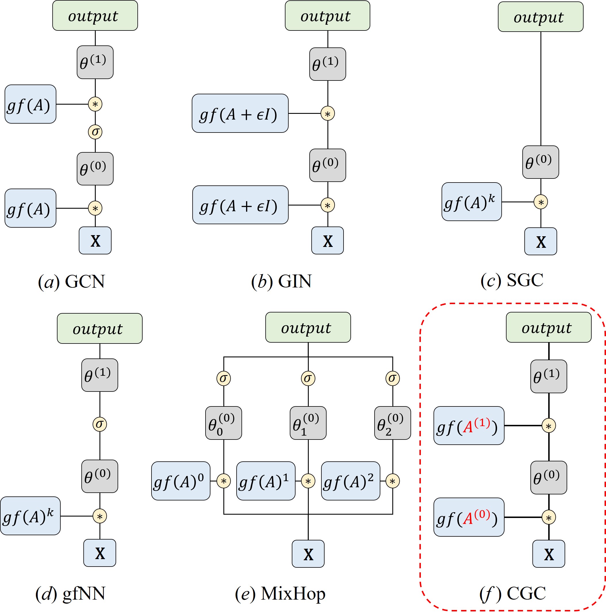
To cope with aforementioned issues, a novel deep learning framework named Coupled Layer-wise Convolutional Recurrent Neural Network (CCRNN) is proposed. Specifically, to address the problem that it is difficult for the popular GCNs to capture multi-level spatial dependence efficiently and accurately, we propose a novel graph convolution architecture, Coupled Layer-wise Graph Convolution (CGC), with self-learned adjacency matrices varying from layer to layer. Figure 1 shows a visual comparison between CGC and several popular graph convolutional networks. Furthermore, by modeling the layer-wise topological structure correlations, we provide a coupled mapping mechanism to implement this graph convolution structure at a small computational cost. The extracted representations are attached different importance by a multi-level aggregation module. Finally, the above components are fused with a recurrent unit to capture spatio-temporal correlations simultaneously. In summary, this paper has the following contributions:
-
•
A novel graph convolution architecture is proposed to extract multi-level spatial dependence adaptively. This structure has different adjacency matrices in different layers and all adjacency matrices are self-learned during the training process.
-
•
A layer-wise coupling mechanism is proposed to bridge the upper-level adjacency matrix with the lower-level one according to the hidden correlations of topological structures in different layers. It also reduces computational costs during the training process.
-
•
A unitary prediction framework is proposed to make the final prediction by integrating the spatial hidden states with gated recurrent unit in a sequence to sequence architecture, where the spatial hidden states are obtained by aggregating multi-level demand dependence.
Related Work
In this section, we review the literature related to our work from the perspectives of transportation demand prediction and graph convolution.
Transportation Demand Prediction
Huge efforts have been made in traffic prediction due to the years of continuous research. In the early time, the attention was mainly paid to combining data mining methods and empirical statistical analysis (Moreira-Matias et al. 2013; Liu et al. 2016; Tong et al. 2017). Those methods have limited researched region and spatio-temporal correlations could not be captured simultaneously. Deep learning methods provide a new perspective to deal with non-linear relations. Lv et al. (2014) used a SAE (stacking autoencoders) to extract representations. Zhang, Zheng, and Qi (2017) treated the demands in the whole city as an image at each time step, and leveraged popular models in CV field at that time, residual network, to capture correlations between different grids. Following this line, Yao et al. (2018) proposed a multi-view network incorporating CNN and Long Short-Term Memory (LSTM) to capture sptatio-temporal correlations simultaneously. Zhou et al. (2018) clustered the demand snapshots to select representations. Ye et al. (2019) explored the correlations between different modes of transportation and made a co-prediction. However, it is hard for CNN-based methods to capture long-distance transition patterns, which makes graph convolutional network step onto the stage (Yu, Yin, and Zhu 2017; Bai et al. 2019; Yu et al. 2020). Li et al. (2017) unified diffusion convolutional layer with Gated Recurrent Unit (GRU) in an encoder-decoder architecture. Chen et al. (2019) explored the correlations of both nodes and edges with two types adjacency matrices. Yu et al. (2019) proposed a 3D graph convolutional network. It is worth mentioning that Wu et al. (2019b) employed an random initialized adaptive adjacency matrix to capture the hidden spatial dependency precisely. However, it is difficult for grid-based data incorporating with graph convolution based methods to get satisfying results.
Graph Convolutional Network
Graph convolutional network which generalizes convolutional neural network to non-Euclidean data has received increasing attention over past few years. Bruna et al. (2013) extended the convolution network to graph-based data. Defferrard, Bresson, and Vandergheynst (2016) reduced the computational cost with Chebyshev polynomials. A first-order Chebyshev polynomials approximation was introduced by Kipf and Welling (2016).
Graph convolutional networks fall into two main categories, spatial-based and spectral-based (Wu et al. 2020). Spatial-based methods update information by designing different strategies to aggregate features of their neighbors (Hamilton, Ying, and Leskovec 2017). Veličković et al. (2017) employed attention mechanisms to learn weights between two nodes. Spectral-based methods treat graph convolution operation as removing noises from graph signal, and the key to this stream is the structure and capacity of the filter. Along this line, Chiang et al. (2019) weakened the influence of neighbors by adding an identity matrix to adjacency matrix. Xu et al. (2019) enhanced low-frequency filters with the heat kernel. Li et al. (2018) learned an adaptive residual Laplacian matrix with generalized Mahalanobis distance. However, they all leverage the initial adjacency matrix and its variants, which fails to capture multi-level dependence efficiently and accurately.
Preliminaries
In this section, we present several definitions and the problem formalization.
Station-level Demand Prediction
Transportation Station. The modes of transportation could be divided into two categories, station-based and station-less. For the station-based transportation, such as bus and subway, it is intuitive to be formalized as graph structure by denoting each station as a node. For the station-less transportation, such as taxi and sharing bike, although the locations of passengers’ arrival and departure are discrete, they tend to gather around certain places. For example, there are many taxi order requests at the main entrance of a university, which forms a virtual station naturally (Du et al. 2020). Discovering potential stations can help to capture transportation demand features and make predictions more accurately. It is worth mentioning that most recent deep learning based demand prediction methods partition the city into grids to meet the requirement of CNN. We employ a Density Peak Clustering (DPC) (Rodriguez and Laio 2014) based method to discover virtual stations.
Adjacency Matrix. Given a graph , we denote as the set of nodes and as the set of edges. In the transportation system, the stations correspond to the nodes in study regions. At time step , the graph has a feature matrix where is the input feature dimension and is the number of nodes. Given graph signals of time steps, we aim at obtaining an adjacency matrix with a data-driven method to complete the definition of . The mapping function is described as:
| (1) |
where denotes the first time step in this adjacency matrix generating problem.
Transportation Demand Prediction. At time step , given the graph and steps historical graph signals, we intend to obtain a mapping function to forecast next steps graph signals. This can be defined as:
| (2) |
where and .
Graph Convolutional Network
Given a graph , we denote as the normalized adjacency matrix:
| (3) |
where is the adjacency matrix, is a diagonal matrix of node degrees, . Following (Li et al. 2017), we remove the activation function and model the diffusion process with steps under undirected graph structure, which leads to the final feature propagation equation:
| (4) |
where is the filter with the parameters , and is the input signals.
An Unifying View of the Existing GCNs. Spectral-based graph convolutional network research mainly focuses on the definition of convolution filter . As illustrated in Figure 1, (a) GCN introduces a first-order Chebyshev polynomials filter approximation (Kipf and Welling 2016), which has been widely adopted; (b) GIN (Graph Isomorphism Network) is constructed with an added weighted identity matrix on the adjacency matrix (Xu et al. 2018). They proved graph convolutional network is as powerful as Weisfeiler-Lehman (WL) graph isomorphism test (Weisfeiler and Lehman 1968); (c) SGC (Simple Graph Convolution) simplifies the multi-layer graph convolutional network by multiplying the initial adjacency matrix by itself times (Wu et al. 2019a); (d) gfNN (graph filter Neural Network) adds an activation function and a mapping function on the basis of SGC in order to model non-linear correlations (NT and Maehara 2019); (e) MixHop explores the latent representations of the immediate neighbors and further neighbors by mixed powers of the adjacency matrix (Abu-El-Haija et al. 2019).
Those researches employed graph convolution with the initial adjacency matrix and its high powers, which makes it difficult to capture multi-level dependence efficiently. As shown in Table 1 (f), to address this problem, CGC extracts the hierarchical representations with self-learned adjacency matrices varying from layer to layer.
Methodology
In this section, we introduce the details of CCRNN. Figure 2 shows the architecture of our proposed method.
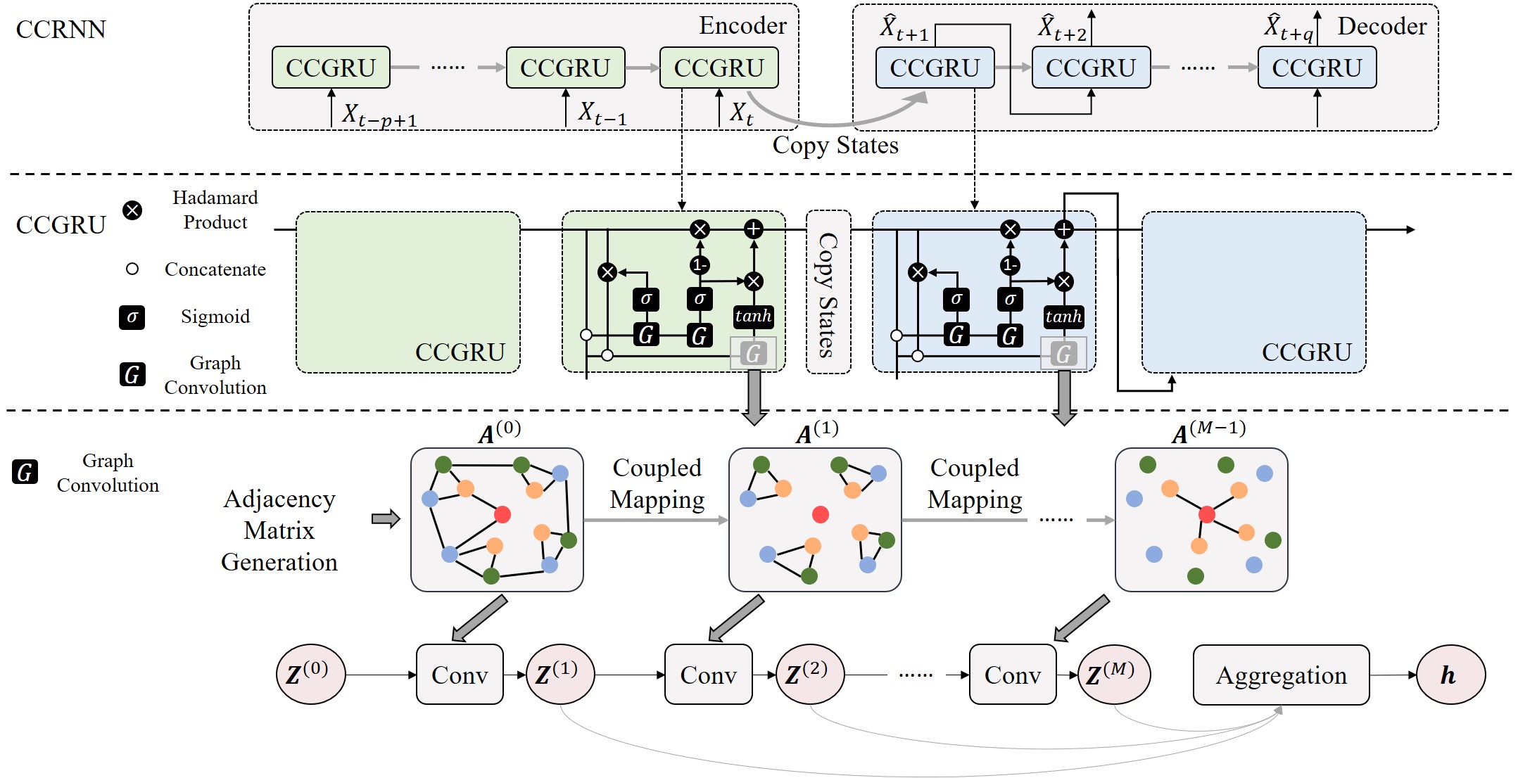
Adjacency Matrix Generation
Adjacency matrix is crucial as it determines the aggregation manner of nodes themselves and their neighbors in graph convolution. Different from the proposed methods which use hand-designed features to construct the graph structure in advance, our adjacency matrix generation method is totally data-driven, and temporal correlations are extracted.
Given a set of graph signals , we reshape this 3-D tensor as a 2-D matrix shaped . To capture interior similarity between different stations and filter the redundant information among stations, we decompose the 2-D matrix into two:
| (5) |
where indicate the time-wise and station-wise matrices. Actually, we use Singular Value Decomposition (SVD) to decompose in experiments.
A large number of repeated transportation patterns are hidden in . SVD could filter the redundant information out by dimension reduction. contains the compact and high-level representations of each station, where is the dimension of the stations’ features. We calculate the similarity of -th and -th rows of as their edge weight in adjacency matrix:
| (6) |
where indicates the -th row and -th column of the adjacency matrix . Here we use the Gaussian kernel based method to estimate the pairwise similarity. The Equation (6) can be redefined as:
| (7) |
where is the standard deviation.
Coupled Layer-wise Graph Convolution
Previous works partition the city into regular grids to meet the requirement of CNN, but the fixed and local receptive field of CNN makes it hard to capture the features of long-distance transition and the similarity between regions. The theory of spectral graph generalizes the convolution operation from regular gird structure to graph structure. However, it is still unwise to use graph convolution on gird-based data to extract high-level representations of each time step to make precise predictions, because there might be multiple modes of transportation patterns mixed together in one gird simultaneously. To address this problem, we introduce a unified graph formalization for station-based and station-less transportations.
To capture multi-level dependence efficiently and accurately, we propose a novel graph convolutional network, Coupled Layer-wise Graph Convolution (CGC), which has different adjacency matrices in different layers. This structure can be defined recursively:
| (8) |
where represents the input of layer . is not only the output of layer but also the input of layer . The multi-level relationship of nodes is modeled by which varies from layer to layer. We use a coupled mapping function to construct upper-level adjacency matrix in layer :
| (9) |
Self-adaptive convolution multiplies two random initial matrices which does not require any prior knowledge and matrices are trained end-to-end through stochastic gradient descent (Wu et al. 2019b). In this way, a new adjacency matrix is generated to extract hidden spatial dependencies. However, random initialization brings the difficulty of convergence and numerical instability. To solve this problem, we initialize the self-adaptive matrix with original graph structure and employ stochastic gradient descent to optimize it. The first layer of CGC is defined as:
| (10) |
where . The feature matrix at each time step is fed into the first layer of CGC as input. In this paper, we employ Equation (3) to normalize the adjacency matrix generated by Equation (6). The output is taken as original , and we optimize it with stochastic gradient descent to discover the real spatial relationships.
However, due to the huge number of nodes, adjacency matrix and obtain high computational costs, which lead to the over-parameterization in above formulations. To solve this problem, we decompose into two small matrices with SVD:
| (11) |
where is the source node embedding in the first layer, is the target node embedding, and is the representation dimension. The number of trainable parameters is reduced from to (). Equation (10) can be redefined as:
| (12) |
Additionally, function is implemented by fully connected layer to model the layer-wise correlations. We share the parameters of fully connected layers between and :
| (13) | ||||
where and denote the source node embedding and target node embedding in -th layer. and represent the weight and bias. To simplify the model, the feature dimensions of and in different layers are all set as . The parameter number of each coupled mapping is reduced to .
Multi-level Aggregation
For gathering the information from all graph convolution layers rather than extracting from only one fixed layer, we implement the multi-level aggregation by an attention mechanism to select the information which is relatively important to the current prediction task.
Graph signals’ multi-level representations obtained by CGC are denoted as , , where represents the total number of graph convolution layers, and denotes the dimension of features. The attention scores are calculated by a linear transformation, and Softmax function helps to normalize the coefficients. With summing up the outputs of multiplying the and normalized scores, the aggregation is defined as:
| (15) |
| (16) |
where and represent the weight and bias in linear transformation, is the flattened version of , and is the attention score of . is the final result of CGC, and the output will be fed into GRU.
Temporal Dependence Modeling
GRU, a simple but powerful variant of RNN, solves the problem of exploding and vanishing gradient. Following (Li et al. 2017), we replace the linear transformation in GRU with the combination of CGC and multi-level aggregation. The Coupled Layer-wise Convolutional Recurrent Gated Recurrent Unit (CCGRU) is defined as:
| (17) | ||||
where and represent the result of attention mechanism and output of GRU at time step. is the Hadamard product, and is the Sigmoid function. Reset gate helps to forget dispensable information, and the update gate controls the output of GRU at time step . We denote the convolution operation in Equation (14) as , and represent the parameters of corresponding filters.
In multi-step forecasting model, we employ the sequence to sequence architecture and scheduled sampling strategy (Li et al. 2017). During the training period, the final state of the encoder is copied to initialize the decoder, and the decoder obtains previous ground truth in a decaying probability to predict. The forecasting results replace the ground truth observations in the testing step. Along with the last piece of the puzzle, we finish building Coupled Layer-wise Convolutional Recurrent Neural Network (CCRNN).
Experiments
| Method | NYC Citi Bike | NYC Taxi | ||||
| RMSE | MAE | PCC | RMSE | MAE | PCC | |
| HA | 5.2003 | 3.4617 | 0.1669 | 29.7806 | 16.1509 | 0.6339 |
| XGBoost (Chen and Guestrin 2016) | 4.0494 | 2.4690 | 0.4861 | 21.1994 | 11.6806 | 0.8077 |
| FC-LSTM (Hochreiter and Schmidhuber 1997) | 3.8139 | 2.3026 | 0.5675 | 18.0708 | 10.2200 | 0.8645 |
| DCRNN (Li et al. 2017) | 3.2094 | 1.8954 | 0.7227 | 14.7926 | 8.4274 | 0.9122 |
| STGCN (Yu, Yin, and Zhu 2017) | 3.6042 | 2.7605 | 0.7316 | 22.6489 | 18.4551 | 0.9156 |
| STG2Seq (Bai et al. 2019) | 3.9843 | 2.4976 | 0.5152 | 18.0450 | 9.9415 | 0.8650 |
| Graph WaveNet (Wu et al. 2019b) | 3.2943 | 1.9911 | 0.7003 | 13.0729 | 8.1037 | 0.9322 |
| CCRNN | 2.8382 | 1.7404 | 0.7934 | 9.5631 | 5.4979 | 0.9648 |
In this section, experimental results and detailed analysis will be presented. The source code is available 111https://github.com/Essaim/CGCDemandPrediction.
Datasets
Experiments are conducted on two real-world datasets collected from NYC OpenData. The two datasets contain order records of taxi and bike in NYC.
-
•
NYC Citi Bike222https://www.citibikenyc.com/system-data: This dataset includes the NYC Citi bike orders of people daily using. We choose the transaction records from April , 2016 to June , 2016 (91 days). Following information is contained: bike pick-up station, bike drop-off station, bike pick-up time, bike drop-off time, trip duration.
-
•
NYC Taxi333https://www1.nyc.gov/site/tlc/about/tlc-trip-record-data.page: This dataset consists of 35 million taxicab trip records in New York from April , 2016 to June , 2016. Following information is contained: pick-up time, drop-off time, pick-up longitude, pick-up latitude, drop-off longitude, drop-off latitude, trip distance.
Baselines
Following methods are compared and we tune the key hyper-parameters to make sure that they have the best performance.
-
•
HA: We calculate the average of historical values at previous time steps as history average.
-
•
XGBoost: XGBoost (Chen and Guestrin 2016) is a widely used method based on gradient boosting tree.
-
•
FC-LSTM: LSTM (Hochreiter and Schmidhuber 1997) incorporates with fully connected network.
-
•
DCRNN: Diffusion convolution recurrent neural network (Li et al. 2017) combines diffusion graph convolution with GRU in an encoder-decoder manner.
-
•
STGCN: Spatial-temporal graph convolution network (Yu, Yin, and Zhu 2017) combines graph convolution with casual convolution.
-
•
STG2Seq: Spatial-temporal graph to sequence model (Bai et al. 2019) can capture the long-term and the short-term information.
-
•
Graph WaveNet: Graph WaveNet (Wu et al. 2019b) conducts graph convolution with adaptive adjacency matrix.
Experimental Setup
The researched region is an rectangle covering West New York, Manhattan Island and part of Brooklyn. NYC Citi Bike is dock-based and every depot of bikes is considered as a station. We filter out the stations with fewer orders and keep the 250 stations with the most orders. As for dockless NYC Taxi, their orders are clustered into 266 virtual stations. The time step length is set to half an hour, such as to , to , to . Among the last four weeks, the first two are used for validation, and the last two are for testing.
The demands in all stations are standardized. The feature dimension is 2, representing the pick-up demand and drop-off demand. The historical demand length is set to 12 and the prediction length is 12, too. In the adjacency matrix generation, to avoid the influence of validation and testing data, we employ the entire training dataset to learn stations’ representations. That is to say, the first time step of generating adjacency matrix is 0, and the length is 3,011 (the length of training set). The dimension of station feature is set to 20. In CGC, the number of stacked convolution layers is 3. We use Equation (14) as final convolution layer with diffusion steps . The dimension of two adaptive matrices is 50. The hidden states dimension is set to 25. Learning rates for NYC Citi Bike and NYC Taxi datasets are 0.0005 and 0.0015. For training stability, we initialize the weight as identity matrix and bias as 0 in coupled mapping. All methods are optimized by Adam algorithm (Kingma and Ba 2014). The model is implemented with the PyTorch framework. We choose the following three evaluation metrics: Root Mean Squared Error (RMSE), Mean Absolute Error (MAE), and Pearson Correlation Coefficient (PCC). RMSE between the output and the ground truth is used as the loss function.
Main Results
Comparison with Baselines. Table 1 shows the comparison results with different baselines. We evaluate models on the multi-step outputs to obtain a global view. Each baseline is trained for 10 times to obtain an average result. Compared with the performances on NYC Taxi, methods have relatively smaller RMSE in NYC Citi Bike since NYC Taxi has a larger demand number. Our method achieves the best performance in all evaluation metrics on two datasets.
Poor performances of HA, XGBoost, FC-LSTM indicate the limitation of employing temporal correlations only. Although STGCN has a bigger RMSE than XGBoost on NYC Taxi, the outputs of STGCN show relatively high correlations on both two datasets. STG2Seq is a novel multi-step demand prediction architecture which combines long-term and short-term dependencies with attention mechanism. However, the zero padding for capturing spatial and temporal correlations simultaneously with simple graph convolution component might lead to the unsatisfactory results for STG2Seq. Combining the sequence to sequence architecture for time series prediction with graph convolution contributes to the good performance of DCRNN. Benefit from adaptive adjacency matrix learning, Graph WaveNet also has competitive results. Our method achieves and RMSE lower than Graph WaveNet on two datasets, which indicates CCRNN captures transportation demand dependencies more accurately and efficiently.
Performances on Multi-step Demand Prediction. In the section, we illustrate the superiority of our model on single step prediction. Because of the space limitation, we evaluate our methods with several baselines at four specific time steps. As it is shown in Figure 3, we choose the first step (0.5 hour), the last step (6.0 hour), and two middle steps (2.5 hour and 4.5 hour).
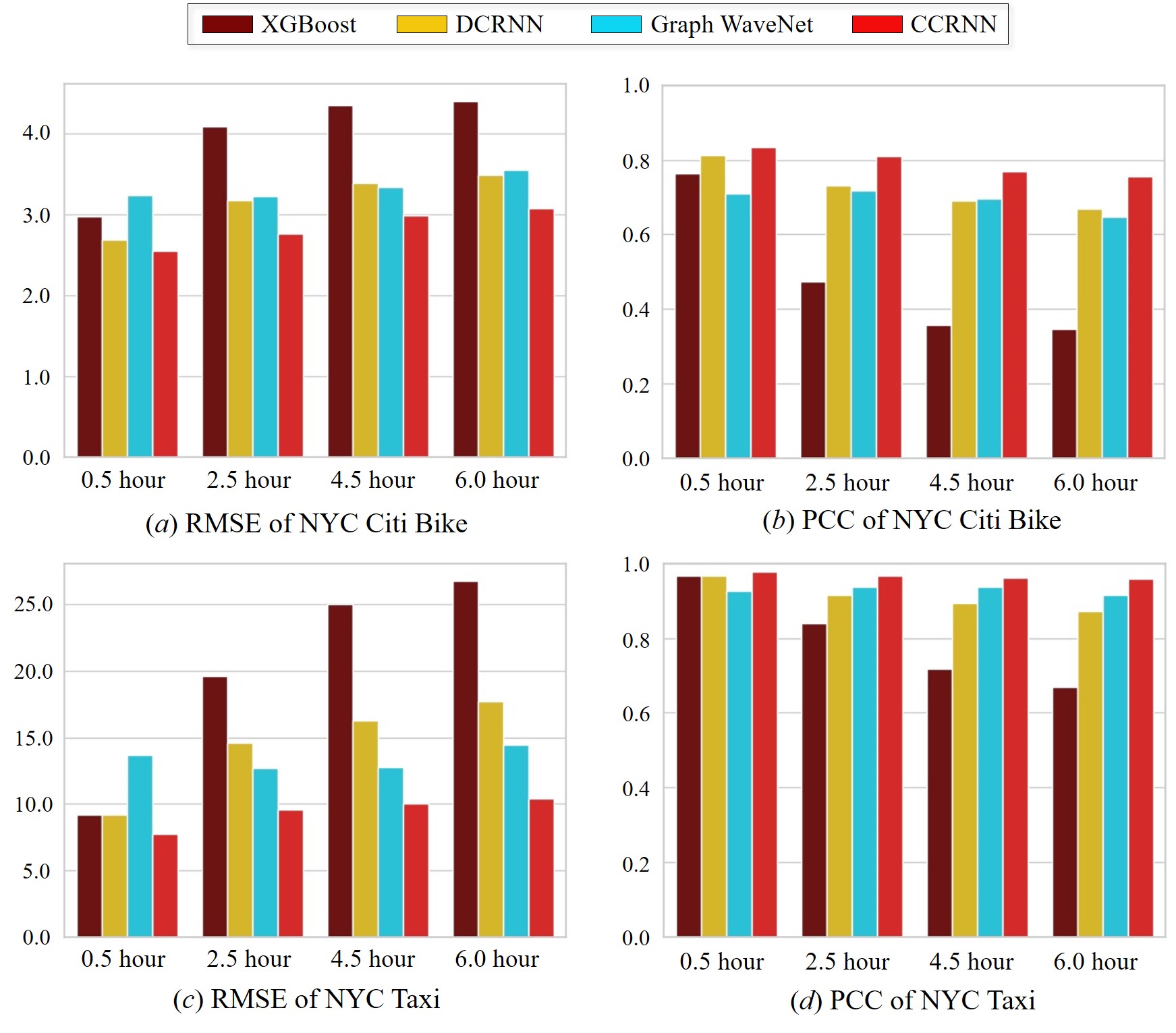
XGBoost has the worst performance in middle-term and long-term predictions (2.5 hour, 4.5 hour and 6.0 hour) since its ignorance of spatial correlations. Due to the recurrent prediction architecture, the performance of DCRNN declines as the forecast time becomes longer. Graph WaveNet outputs multi-step demands at once, which leads to stable results at different time steps, but relatively lower accuracy in short-term prediction (0.5 hour). Although our model is in a sequence to sequence manner and suffers from the performance declining, we achieve the lowest RMSE and the highest PCC.
Ablation Study
We conduct an detailed ablation study on our method by removing or changing several components. In particular, five variants of our model are obtained by 1) No Adaptive: setting and untrainable, 2) No Coupling: removing the coupled mapping, 3) Random Init: randomly initializing and , 4) Distance Init: initializing with the distance between nodes (Li et al. 2017), 5) PCC Init: initializing with PCC of demand time series (Bai et al. 2019).
As it is shown in Table 2, we could make a conclusion that the complete CCRNN achieves the best performance and the adjacency matrix generated by our method contains the most information. The adaptive and coupled layer-wise matrices help our model discover more accurate connectivity information and obtain high-level representations more efficiently. Benefit from those components, although the variants initialized by the distance between stations and PCC of the time series obtain higher RMSE than CCRNN, their performances outperform all baselines in Table 1. Randomly initializing and leads to the poor performances with PCC lower than . It is necessary for our method to get the adjacency matrix initialized properly to guide training.
| Method | RMSE | MAE | PCC | |
| NYC Citi Bike | No Adaptive | 3.2648 | 1.9157 | 0.7143 |
| No Coupling | 3.0555 | 1.8217 | 0.7702 | |
| Random Init. | 4.7308 | 3.0366 | 0.0204 | |
| Distance Init. | 2.9718 | 1.7995 | 0.7768 | |
| PCC Init. | 2.9096 | 1.7729 | 0.7851 | |
| CCRNN | 2.8382 | 1.7404 | 0.7934 | |
| NYC Taxi | No Adaptive | 12.0516 | 7.2842 | 0.9404 |
| No Coupling | 10.1864 | 5.8168 | 0.9594 | |
| Random Init. | 36.0307 | 22.2210 | 0.0065 | |
| Distance Init. | 10.6882 | 6.1476 | 0.9559 | |
| PCC Init. | 10.0244 | 5.7927 | 0.9619 | |
| CCRNN | 9.5631 | 5.4979 | 0.9648 |
Conclusion
In this paper, we presented a novel transportation demand prediction model, namely, CCRNN. In particular, to capture multi-level spatial dependence, we proposed a novel graph convolution architecture, CGC. The adjacency matrices in CGC were self-learned and varied from layer to layer. Furthermore, a layer-wise coupling mechanism was employed to bridge the upper-level graph structure with the lower-level one. It also reduced the scale of parameters in our model. Then, the different importance was attached to extracted representations by a multi-level aggregation module. A unitary network fused the above components to make final predictions. Experiments were conducted on real-world taxi and sharing bike datasets, and state-of-the-art results were achieved by CCRNN. This research represented a new perspective in graph convolutional network with layer-wise adjacency matrices. In the future, we will study performances of CGC on other graph convolution tasks.
Acknowledgments
This work is supported by the National Natural Science Foundation of China under Grant No. 51778033, 51822802, 51991395, 71901011, U1811463, the National Key R&D Program of China No. 2018YFB2101003, the Science and Technology Major Project of Beijing under Grant No. Z191100002519012.
References
- Abu-El-Haija et al. (2019) Abu-El-Haija, S.; Perozzi, B.; Kapoor, A.; Alipourfard, N.; Lerman, K.; Harutyunyan, H.; Ver Steeg, G.; and Galstyan, A. 2019. MixHop: Higher-Order Graph Convolutional Architectures via Sparsified Neighborhood Mixing. In International Conference on Machine Learning, 21–29.
- Bai et al. (2019) Bai, L.; Yao, L.; Kanhere, S. S.; Wang, X.; and Sheng, Q. Z. 2019. STG2seq: spatial-temporal graph to sequence model for multi-step passenger demand forecasting. In Proceedings of the 28th International Joint Conference on Artificial Intelligence, 1981–1987. AAAI Press.
- Bruna et al. (2013) Bruna, J.; Zaremba, W.; Szlam, A.; and LeCun, Y. 2013. Spectral networks and locally connected networks on graphs. arXiv preprint arXiv:1312.6203 .
- Chen and Guestrin (2016) Chen, T.; and Guestrin, C. 2016. Xgboost: A scalable tree boosting system. In Proceedings of the 22nd acm sigkdd international conference on knowledge discovery and data mining, 785–794.
- Chen et al. (2019) Chen, W.; Chen, L.; Xie, Y.; Cao, W.; Gao, Y.; and Feng, X. 2019. Multi-range attentive bicomponent graph convolutional network for traffic forecasting. arXiv preprint arXiv:1911.12093 .
- Chiang et al. (2019) Chiang, W.-L.; Liu, X.; Si, S.; Li, Y.; Bengio, S.; and Hsieh, C.-J. 2019. Cluster-gcn: An efficient algorithm for training deep and large graph convolutional networks. In Proceedings of the 25th ACM SIGKDD International Conference on Knowledge Discovery & Data Mining, 257–266.
- Defferrard, Bresson, and Vandergheynst (2016) Defferrard, M.; Bresson, X.; and Vandergheynst, P. 2016. Convolutional neural networks on graphs with fast localized spectral filtering. In Advances in neural information processing systems, 3844–3852.
- Du et al. (2020) Du, B.; Hu, X.; Sun, L.; Liu, J.; Qiao, Y.; and Lv, W. 2020. Traffic Demand Prediction Based on Dynamic Transition Convolutional Neural Network. IEEE Transactions on Intelligent Transportation Systems .
- Hamilton, Ying, and Leskovec (2017) Hamilton, W.; Ying, Z.; and Leskovec, J. 2017. Inductive representation learning on large graphs. In Advances in neural information processing systems, 1024–1034.
- Hochreiter and Schmidhuber (1997) Hochreiter, S.; and Schmidhuber, J. 1997. Long short-term memory. Neural computation 9(8): 1735–1780.
- Kingma and Ba (2014) Kingma, D. P.; and Ba, J. 2014. Adam: A method for stochastic optimization. arXiv preprint arXiv:1412.6980 .
- Kipf and Welling (2016) Kipf, T. N.; and Welling, M. 2016. Semi-supervised classification with graph convolutional networks. arXiv preprint arXiv:1609.02907 .
- Li et al. (2018) Li, R.; Wang, S.; Zhu, F.; and Huang, J. 2018. Adaptive graph convolutional neural networks. In Thirty-second AAAI conference on artificial intelligence.
- Li et al. (2017) Li, Y.; Yu, R.; Shahabi, C.; and Liu, Y. 2017. Diffusion convolutional recurrent neural network: Data-driven traffic forecasting. arXiv preprint arXiv:1707.01926 .
- Liu et al. (2016) Liu, J.; Sun, L.; Chen, W.; and Xiong, H. 2016. Rebalancing bike sharing systems: A multi-source data smart optimization. In Proceedings of the 22nd ACM SIGKDD International Conference on Knowledge Discovery and Data Mining, 1005–1014.
- Lv et al. (2014) Lv, Y.; Duan, Y.; Kang, W.; Li, Z.; and Wang, F.-Y. 2014. Traffic flow prediction with big data: a deep learning approach. IEEE Transactions on Intelligent Transportation Systems 16(2): 865–873.
- Moreira-Matias et al. (2013) Moreira-Matias, L.; Gama, J.; Ferreira, M.; Mendes-Moreira, J.; and Damas, L. 2013. Predicting taxi–passenger demand using streaming data. IEEE Transactions on Intelligent Transportation Systems 14(3): 1393–1402.
- NT and Maehara (2019) NT, H.; and Maehara, T. 2019. Revisiting Graph Neural Networks: All We Have is Low-Pass Filters. arXiv preprint arXiv:1905.09550 .
- Rodriguez and Laio (2014) Rodriguez, A.; and Laio, A. 2014. Clustering by fast search and find of density peaks. Science 344(6191): 1492–1496.
- Tong et al. (2017) Tong, Y.; Chen, Y.; Zhou, Z.; Chen, L.; Wang, J.; Yang, Q.; Ye, J.; and Lv, W. 2017. The simpler the better: a unified approach to predicting original taxi demands based on large-scale online platforms. In Proceedings of the 23rd ACM SIGKDD international conference on knowledge discovery and data mining, 1653–1662.
- Veličković et al. (2017) Veličković, P.; Cucurull, G.; Casanova, A.; Romero, A.; Lio, P.; and Bengio, Y. 2017. Graph attention networks. arXiv preprint arXiv:1710.10903 .
- Weisfeiler and Lehman (1968) Weisfeiler, B.; and Lehman, A. A. 1968. A reduction of a graph to a canonical form and an algebra arising during this reduction. Nauchno-Technicheskaya Informatsia 2(9): 12–16.
- Wu et al. (2019a) Wu, F.; Souza Jr, A. H.; Zhang, T.; Fifty, C.; Yu, T.; and Weinberger, K. Q. 2019a. Simplifying Graph Convolutional Networks. In ICML.
- Wu et al. (2020) Wu, Z.; Pan, S.; Chen, F.; Long, G.; Zhang, C.; and Philip, S. Y. 2020. A comprehensive survey on graph neural networks. IEEE Transactions on Neural Networks and Learning Systems .
- Wu et al. (2019b) Wu, Z.; Pan, S.; Long, G.; Jiang, J.; and Zhang, C. 2019b. Graph wavenet for deep spatial-temporal graph modeling. In Proceedings of the 28th International Joint Conference on Artificial Intelligence, 1907–1913. AAAI Press.
- Xu et al. (2019) Xu, B.; Shen, H.; Cao, Q.; Cen, K.; and Cheng, X. 2019. Graph convolutional networks using heat kernel for semi-supervised learning. In Proceedings of the 28th International Joint Conference on Artificial Intelligence, 1928–1934. AAAI Press.
- Xu et al. (2018) Xu, K.; Hu, W.; Leskovec, J.; and Jegelka, S. 2018. How Powerful are Graph Neural Networks? In International Conference on Learning Representations.
- Yao et al. (2018) Yao, H.; Wu, F.; Ke, J.; Tang, X.; Jia, Y.; Lu, S.; Gong, P.; Ye, J.; and Li, Z. 2018. Deep multi-view spatial-temporal network for taxi demand prediction. In Thirty-Second AAAI Conference on Artificial Intelligence.
- Ye et al. (2019) Ye, J.; Sun, L.; Du, B.; Fu, Y.; Tong, X.; and Xiong, H. 2019. Co-Prediction of Multiple Transportation Demands Based on Deep Spatio-Temporal Neural Network. In Proceedings of the 25th ACM SIGKDD International Conference on Knowledge Discovery & Data Mining, 305–313.
- Yu et al. (2019) Yu, B.; Li, M.; Zhang, J.; and Zhu, Z. 2019. 3d graph convolutional networks with temporal graphs: A spatial information free framework for traffic forecasting. arXiv preprint arXiv:1903.00919 .
- Yu, Yin, and Zhu (2017) Yu, B.; Yin, H.; and Zhu, Z. 2017. Spatio-temporal graph convolutional networks: A deep learning framework for traffic forecasting. arXiv preprint arXiv:1709.04875 .
- Yu et al. (2020) Yu, L.; Du, B.; Hu, X.; Sun, L.; Han, L.; and Lv, W. 2020. Deep spatio-temporal graph convolutional network for traffic accident prediction. Neurocomputing 423: 135–147.
- Zhang, Zheng, and Qi (2017) Zhang, J.; Zheng, Y.; and Qi, D. 2017. Deep spatio-temporal residual networks for citywide crowd flows prediction. In Thirty-First AAAI Conference on Artificial Intelligence.
- Zhou et al. (2018) Zhou, X.; Shen, Y.; Zhu, Y.; and Huang, L. 2018. Predicting multi-step citywide passenger demands using attention-based neural networks. In Proceedings of the Eleventh ACM International Conference on Web Search and Data Mining, 736–744.