Coupled Time-lapse Full Waveform Inversion for Subsurface Flow Problems using Intrusive Automatic Differentiation
Abstract
We describe a novel framework for estimating subsurface properties, such as rock permeability and porosity, from time-lapse observed seismic data by coupling full-waveform inversion, subsurface flow processes, and rock physics models.. For the inverse modeling, we handle the back-propagation of gradients by an intrusive automatic differentiation strategy that offers three levels of user control: (1) at the wave physics level, we adopted the discrete adjoint method in order to use our existing high-performance FWI code; (2) at the rock physics level, we used built-in operators from the TensorFlow backend; (3) at the flow physics level, we implemented customized PDE operators for the potential and nonlinear saturation equations. These three levels of gradient computation strike a good balance between computational efficiency and programming efficiency, and when chained together, constitute a coupled inverse system. We use numerical experiments to demonstrate that (1) the three-level coupled inverse problem is superior in terms of accuracy to a traditional decoupled inversion strategy; (2) it is able to simultaneously invert for parameters in empirical relationships such as the rock physics models; and (3) the inverted model can be used for reservoir performance prediction and reservoir management/optimization purposes.
Water Resources Research
Department of Geophysics, Stanford University, Stanford, CA, 94305 Institute for Computational and Mathematical Engineering, Stanford University, Stanford, CA, 94305 Mechanical Engineering, Stanford University, Stanford, CA, 94305
Dongzhuo Lilidongzh@stanford.edu
We assimilated seismic waveform data to directly invert for hydrological subsurface properties (e.g., permeability).
Coupled inversion leads to more accurate inversion result compared to decoupled inversion.
We adopted an intrusive automatic differentiation strategy with custom operators for high computational efficiency and scalability.
1 Introduction
Accurate inversion for the parameters that govern subsurface flow dynamics plays a vital role in addressing energy and environmental problems, such as oil and gas recovery [Teletzke \BOthers. (\APACyear2010)], storage [Shi \BOthers. (\APACyear2013)], salt-water intrusion [Beaujean \BOthers. (\APACyear2014)], and groundwater contaminant transport [Reid (\APACyear1996), McLaughlin \BBA Townley (\APACyear1996)]. A calibrated flow model can help optimize hydrocarbon production, evaluate environmental risks, and remediate environmental damage.
Conventional direct inversion methods (e.g., history matching [Chen \BOthers. (\APACyear1974), Carter \BOthers. (\APACyear1974), Chavent \BOthers. (\APACyear1975)]) rely on in-situ flow data, such as production history and flow pressure in wells, to fit a flow equation for intrinsic properties such as permeability. However, flow data can only be collected from sparsely distributed wells, and the data are usually integrated along the wellbore. Thus, the inversion suffers from large null-space, and the results exhibit reduced resolution [Yeh (\APACyear1986)].
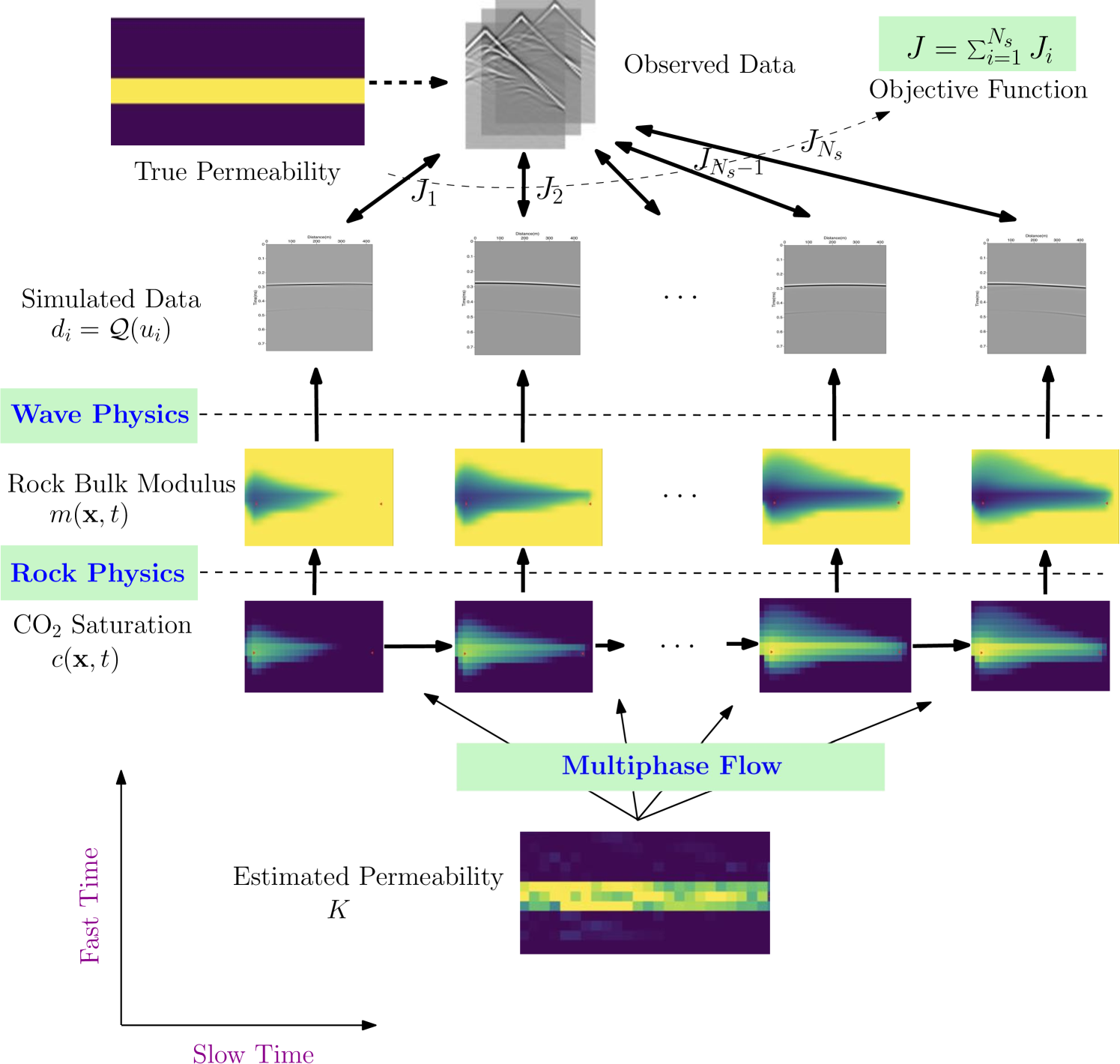
On the other hand, indirect geophysical measurements such as seismic waveform data, provide better volumetric sampling of the reservoir and can reconstruct high-resolution models of elastic properties. The seismic data are collected through time-lapse surveys, e.g., regular or irregular recordings made months or years apart. To be more specific, fast-time refers to the digital sampling interval of the repeated wavefield recordings, whereas slow-time refers to the evolution time or history of flow in a reservoir. The terms, “fast-time” and “slow-time”, are used to emphasize the different time scales for seismic surveys (e.g., days or weeks) and subsurface flow processes (e.g., months or years). In the slow-time case, the flow properties are assumed not to change, or change negligibly, in the short period during which seismic snapshots are recorded. We also assume that intrinsic properties such as permeability and porosity do not change with slow-time.
The main challenge of using seismic data is that they do not directly detect the intrinsic properties of interest. Hence, conventional uses of (time-lapse) seismic data first invert for elastic properties and then treat those intermediate properties as data to estimate intrinsic rock properties. We refer to this strategy as the decoupled inversion, which was for example proposed by \citeArubin1992mapping and \citeAcopty1993geophysical, and was also formulated as the seismic-history matching method [Landa \BOthers. (\APACyear1997), Huang \BOthers. (\APACyear1998), Emerick \BOthers. (\APACyear2007), Volkov \BOthers. (\APACyear2018)]. Although this approach improves the well-posedness of the problem and increases resolution, inaccuracies from the intermediate step of seismic inversion yield artifacts in inverted intrinsic properties [Day-Lewis \BBA Lane Jr (\APACyear2004)].
Besides, the seismic inversion techniques used in subsurface flow problems are usually based on high-frequency approximation (ray theory) and simple linear convolution models. Those methods have the merit of being simple and robust, but they lead to reduced resolution because of limited information used. They also suffer from errors caused by inaccurate physics. Recent developments in FWI have provided great improvements in estimates of elastic properties with high spatial resolution and quantitative accuracy [Tarantola (\APACyear1984), Virieux \BBA Operto (\APACyear2009)]. In hydrogeophysical applications, \citeAklotzsche2012crosshole, \citeAklotzsche2014detection, \citeAgueting2015imaging,gueting2017high, and \citeAkeskinen2017full also find that ground-penetrating radar FWI yields a higher resolution result than ray-based GPR traveltime inversion. Thus, a coupled seismic inversion method fully based on wave equations in line with FWI is highly desirable.
We propose herein a coupled inversion framework that assimilates seismic waveform data to invert for the intrinsic parameters of subsurface flow automatically. This inversion approach combines flow physics, rock physics, and wave physics models. We consider a concrete example with the following three key physical components:
-
1.
slow-time subsurface flow model : an immiscible incompressible two-phase flow model that maps permeability to evolution of fluid saturation and pressure;
-
2.
rock physics model : a patchy-saturation model or a Gassmann’s model that maps saturation to rock elastic properties;
-
3.
fast-time seismic wave physics model : elastic wave propagation that maps elastic properties to seismic waveforms recorded at receiver arrays.
In the field of hydrogeophysics, there has also been substantial research on the coupled inversion [Linde \BBA Doetsch (\APACyear2016)]. In near-surface surveys, the geophysical data are usually electrical resistance tomography (ERT) data or ground penetrating radar (GPR) traveltime. The subsurface flow processes are often tracer dynamics in steady flow [Irving \BBA Singha (\APACyear2010), Pollock \BBA Cirpka (\APACyear2010), Jardani \BOthers. (\APACyear2013)] and unsaturated flow in the vadoes zone [Kowalsky \BOthers. (\APACyear2004), Kowalsky \BOthers. (\APACyear2005), Hinnell \BOthers. (\APACyear2010), Huisman \BOthers. (\APACyear2010)]. Petrophysical models such as Archie’s law [Archie \BOthers. (\APACyear1942)] interlink the hydrological flow properties and geophysical properties. In the above examples, the geophysical forward modeling is not transient by nature or simplified as so. For example, the ERT modeling is governed by the Poisson equation, and the GPR traveltime is computed by (straight) ray tracing [Kowalsky \BOthers. (\APACyear2004), Kowalsky \BOthers. (\APACyear2005)]. Sometimes the transient flow equation is also transformed into a steady-state equation [Pollock \BBA Cirpka (\APACyear2010), Pollock \BBA Cirpka (\APACyear2012)] to reduce the computation complexities. In our formulation, however, both the subsurface flow and the wave propagation are governed by time-dependent PDEs. The complex coupling makes it challenging to use the adjoint-state method [Sun \BBA Yeh (\APACyear1990)]. Since our problem is inherently large-scale, it is also infeasible to use sampling-based methods or global optimization methods as many of the above examples did.
To meet this computational challenge, we propose an intrusive automatic differentiation method to solve this coupled inversion problem with high computational efficiency and scalability. We formulate the inverse problem as a large-scale partial-differential-equation (PDE) constrained optimization problem to be solved by gradient-based optimization methods. However, deriving and implementing the gradients for this coupled system are both nontrivial and laborious. To overcome this difficulty, we develop an automatic-differentiation-based method, intrusive automatic differentiation (IAD), which allows for computing gradients algorithmically and accurately. Our automatic-differentiation-based method is intrusive in the sense that we incorporate customized gradient back-propagation implementations, such as adjoint state or checkpointing schemes codes, into an automatic differentiation framework. This technique allows for gradient back-propagation of custom-designed PDE solvers, even for implicit solvers, which typical automatic differentiation tools cannot handle. Another advantage of IAD is that the custom operators, such as a GPU-accelerated FWI module, enables high performance large-scale scientific computing. This set of tools will potentially benefit researchers in the hydrological community, as well as the inverse modeling community in a broader context.
In numerical examples, we follow a setup in sequestration, in which supercritical is injected into a reservoir filled with water. We show in those examples that
-
1.
coupled inversion is more accurate than the traditional decoupled inversion, and
-
2.
the inversion can simultaneously invert for empirical closure relationship (e.g., the rock physics model parameters) and intrinsic parameters.
The paper is organized as follows. We first describe the general mathematical formulation of the PDE-constrained inversion problem and coupled physics models. Next, we present the intrusive automatic differentiation method. Finally, we conduct numerical examples, discuss, and offer conclusions.
2 Problem Setup
In this section, we first give a general formulation of the coupled full-waveform inversion method for parameters in dynamic geophysical processes. We then discuss in detail the governing equation for the wave propagation and two-phase flow in porous media along with the rock physics that couple flow physics to wave physics.
2.1 General Formulation
The problm is formulated as a PDE-constrained inverse problem. There are two physical processes governed by different PDEs. The first process, the slow-time dynamic flow process, is described by the equation
| (1) |
where is the flow property, i.e., fluid saturation, is the intrinsic rock property, i.e., permeability. Fluid saturation will affect the elastic properties , e.g., rock bulk modulus and density through a closure relationship from the rock physics model :
| (2) |
The slow-time flow process is monitored indirectly within measurements of duration , where is the starting slow-time of the -th measurement and is the fast time interval. Each measurement is a seismic survey conducted by sequentially exciting sources and recording seismic data at corresponding receiver positions. We can also compute predictions of wavefield by solving the wave equation in the first-order velocity-stress form
| (3) |
with as the assumed parameter. Here is the wavefield, which for example can be the field of particle velocity or stress. The time duration of the process Eq. (3) is short compared to Eq. (1), i.e., and therefore we assume that is fixed during and denote . The fast-time scale equation reduces to
| (4) |
In the same manner of recording observed data, we sample the synthetic wavefield with operator : . We can then compute the misfit of synthetic data and observed data as .
Putting together the above equations with proper boundary and initial conditions and , we have
| (5) | |||||
| (6) | |||||
| (7) | |||||
| (8) | |||||
| (9) | |||||
The coupled inversion is schematically illustrated in Fig. 1.
2.2 Multi-phase Flow in Porous Media
The physics of multi-phase flow in porous media is fundamental to many geoscience fields, such as hydrology, reservoir engineering, glaciology, and volcanology. It underlies the slow-time-scale processes of geophysical time-lapse monitoring problems. As an example, we use the physical model of two-phase immiscible incompressible flow in this paper. This model can describe, at least to the first order, the phenomenon of the displacement of one fluid of the other. Examples include injection of water in a reservoir to produce oil, and injection of supercritical into saline aquifers. All symbols in the this model are listed in Table 1.
| Symbol | Meaning |
|---|---|
| porosity | |
| permeability | |
| relative permeability of fluid | |
| saturation of fluid | |
| pressure of fluid | |
| capillary pressure | |
| potential of fluid | |
| capillary potential | |
| Darcy’s velocity of fluid | |
| total velocity | |
| capillary velocity | |
| density of fluid | |
| viscosity of fluid | |
| mobility of fluid : | |
| total mobility: | |
| injection or production rate of the fluid | |
| gravity constant | |
| vector of the Z-direction |
The governing equations are derived from conservation of mass of each phase, and conservation of momentum or Darcy’s law for each phase. First, we have
| (10) |
where Eq. (10) is the mass balance equation, in which denotes porosity, denotes the saturation of the -th phase, denotes fluid density, denotes the volumetric velocity, and stands for injection or production rates. The saturation of two phases should add up to 1, that is,
| (11) |
In the remainder of the paper, we inject fluid 2 into the reservoir to replace fluid 1.
Darcy’s law yields
| (12) |
where is the permeability tensor, which is simplified as a scalar function of space in our model. is the viscosity, is the fluid pressure, is the gravitational acceleration constant, and is the vector in the downward vertical direction. The relative permeability is written as , which describes how easily one phase flows compared to the other. It is a nonlinear function of saturation of the corresponding phase, such as the Corey model [Corey \BOthers. (\APACyear1954)], the Brooks-Corey model [Brooks \BBA Corey (\APACyear1964)], and the van Genuchten-Mualem model [Mualem (\APACyear1976), Van Genuchten (\APACyear1980)]. Without loss of generality, we adopt a simplified Corey model for numerical experiments as follows
| (13) |
where the residuals or irreducible saturations of the two phases are assumed to be zero and the end-point scaling factor is 1 [Lie (\APACyear2019)]. In practice, one may fit those parameters to measurements. We define mobilities , and the total mobility . To complete the system, we use another equation to describe the relationship between the two phase-pressures as
| (14) |
where is the capillary pressure, a function of the saturation of the wetting phase , but it can be ignored and set to zero in fast-displacement processes.
In a nutshell, the flow physics model maps intrinsic properties to flow properties, for example,
| (15) |
We discuss the details of solving the flow equations in SI 1.1.
2.3 Rock Physics Models
The second component in the physics system is the rock physics model that links flow properties to elastic properties. All symbols in the rock physics model are listed in Table 2. In our example, we construct the relationship between the saturation of the injected fluid to the rock bulk modulus and density :
| (16) |
which are also controlled by the other elastic parameters in the parenthesis. Intuitively, the rock bulk modulus and density change with fluid substitution in the rock pore space, as the original and injected fluids may have different bulk moduli and densities. We first use the patchy saturation model that is commonly used for modeling of injection processes [Mavko \BOthers. (\APACyear2009)], and then examine a Gassmann’s model with Brie’s fluid mixing equation [Brie \BOthers. (\APACyear1995), Mavko \BOthers. (\APACyear2009)]. In both models, we ignore the effects of pressure on the elastic properties. One may find details about those two rock physics models in SI 1.2.
| Symbol | Meaning |
|---|---|
| bulk modulus of rock fully saturated with fluid 1 | |
| bulk modulus of rock fully saturated with fluid 2 | |
| bulk modulus of fluid 1 | |
| bulk modulus of fluid 2 | |
| bulk modulus of rock grains | |
| bulk modulus of fluid mixture | |
| rock shear modulus | |
| P-wave velocity of rock fully saturated with fluid 1 | |
| P-wave velocity of rock fully saturated with fluid 2 | |
| S-wave velocity of rock fully saturated with fluid 1 | |
| S-wave velocity of rock fully saturated with fluid 2 | |
| rock porosity | |
| saturation of fluid 1 | |
| saturation of fluid 2 | |
| density of rock grains | |
| density of fluid 1 | |
| density of fluid 2 | |
| density of rock fully saturated with fluid 1 | |
| density of rock as a function of saturation of fluid 2 | |
| bulk modulus of rock as a function of saturation of fluid 2 |
2.4 The Elastic Wave Equation
The wave phenomenon can be described by the following velocity-stress formulation of the elastic wave equation:
| (17) |
where is the particle velocity vector, is the stress tensor, is the body force, and the repeated index indicates the Einstein summation notation. Density is denoted by and the Lamé parameters are represented by and (shear modulus). The first Lamé parameter and bulk modulus that appears in the rock physics model are connected by
| (18) |
We assume that the depth of the studied area is deep enough so that free surface reflected waves do not appear in the recorded data, and we use convolution perfectly matched layers (CPML) [Martin \BOthers. (\APACyear2008)] on the four boundaries to prevent unrealistic reflected waves.
In summary, the wave physics model maps elastic properties to wavefields:
| (19) |
3 Inversion Method – Intrusive Automatic Differentiation
Automatic differentiation has been successfully used in scientific computing and is one of the major contributors to the success and accessibility of deep-learning technology. Within modern deep-learning frameworks such as TensorFlow [Abadi \BOthers. (\APACyear2016)], there is a suite of built-in differentiable operators (or neural network layers). With those operators, users may construct complex forward mapping functions and automatically obtain gradients. Besides, those frameworks offer high-performance computing options, such as GPU acceleration and graph-based parallelization. Those features are highly desirable when implementing complicated functions such as rock physics models. However, it is computationally inefficient to solve PDEs with these built-in operators or layers. Also, automatic differentiation needs to store intermediate variables for gradient back-propagation, which is also demanding for memory resources.
On the other hand, the so-called adjoint method is widely used for large-scale PDE-constrained inverse problems, such as full-waveform inversion, history matching [R. Li \BOthers. (\APACyear2001), Oliver \BBA Chen (\APACyear2011)], 4D variational weather data assimilation [Wang \BOthers. (\APACyear2001)], ocean model inversion [Marotzke \BOthers. (\APACyear1999)], etc. The adjoint method requires analytic derivations of the adjoint equations and gradients. Here we follow the “discretize-then-optimize” philosophy, which means that one first discretizes the forward equations and then makes the following derivations according to the Lagrange multiplier method. We review the details of the discrete adjoint method in SI 2 and illustrate its application to elastic FWI in SI 4. Once the adjoint equations and formulae of gradients are obtained, one may use various techniques to optimize computation efficiency and reduce the memory footprint. For example, it is not possible to store the whole history of forward wave propagation, so we only store wavefields at the boundaries, and reverse the forward wave equations in time to recompute the forward wavefields. The users can adopt other memory-saving strategies, such as saving a few frequency components [Zhang \BOthers. (\APACyear2018)] or using check-pointing methods [Anderson \BOthers. (\APACyear2012)]. It is possible to apply the discrete adjoint method to the whole subsurface flow FWI problem, but the derivations are time-consuming, error-prone, and inflexible, especially when dealing with systems where there are complicated time-stepping schemes and mappings between variables. After all, the derivations are purely mechanical and should be automated.
Therefore, we propose an intrusive automatic differentiation strategy that provides different levels of customization. It combines native automatic differentiation and the discrete adjoint method, such that we can achieve a good balance between computational efficiency and implementation efficiency or flexibility. This is realized by implementing customized PDE operators with gradient computation capabilities that resemble neural network layers in deep-learning frameworks.
As we show in SI 3, automatic differentiation and discrete adjoint method are equivalent. The only difference is that automatic differentiation requires a specific input-output interface in which we only need to implement two methods for each customized operator:
-
1.
Forward operation : compute the output by solving a PDE:
(20) For example, represents a single-step discrete-time propagation of a wave equation, is the wavefield (a vector of particle velocity and stress) at the -th time step, and is the Lamé parameters. In the general case, can be any state variables of a PDE, and is the PDE parameter, which depends on the physical quantity we want to calibrate.
-
2.
Backward operation : given gradient , compute and with the chain rule. The backward process back-propagates the gradient of the objective function with respect to the output to the input variables:
(21)
Note that only the matrix-vector product needs to be implemented, and there should be no need to construct Jacobian matrices like explicitly.
The customized PDE operators enable two different levels of customization. For example,
-
1.
the forward process can be wave propagation plus misfit computation, and the backward gradient is computed by the adjoint method. In other words, we encapsulate the entire FWI in an operator.
-
2.
the forward process can be a forward step in the numerical solving of PDEs. This level of customization is helpful when the forward step is numerically complicated. For example, in our flow simulations, we solve nonlinear equations with the Newton-Raphson method and use implicit-time stepping.
Specifically, for explicit time-stepping, the implementation of backward is straight-forward, as one can usually derive it from the forward code directly. However, we need to employ special tricks for the implicit time-stepping. Now we consider a problem with implicit constraints:
| (22) | ||||
where the set of equations establish the forward mappings , respectively.
However, the programming interface for backward is still to compute
| (23) |
when we are supplied with .
We compute them using the following technique: Take the partial derivative with respect to the interested parameter (e.g., ) on the constraint equation and obtain
| (24) |
and thus
| (25) |
Therefore,
| (26) |
If we let
| (27) |
then we can get by solving the following linear system
| (28) |
and then can get
| (29) |
To summarize, we (1) solve linear system Eq. (28) for adjoint variables , and (2) compute the matrix-vector product as in Eq. (29).
Example.
Consider the following constrained optimization problem
| (30) | ||||
| (31) |
where is a scalar parameter to be calibrated, is the state variable of a PDE whose discrete form is given by , is the observation vector, is a known source term, and is the coefficient matrix whose entries depend on . Our goal is to compute the derivative of
where is the solution to the constraint , i.e., .
Let
Using Equation 26, we have (subtitute with , with , and with )
In the essence of Equation 28, we first calculate by solving the linear system
and finally we have
In the intrusive automatic differentiation, this process can be incorporated into an automatic differentiation system and therefore exchanges state variable and gradient information with other physical modules. For more implementation details, see our software FwiFlow.jl and the supporting information (SI) material.
4 Numerical Experiments
4.1 Coupled vs. Decoupled Inversion
Our examples are inspired by sequestration projects for the reduction of emission into the atmosphere. In this example, an injection well injects super-critical at a constant rate. It would be more accurate to implement a constant-flow-rate boundary condition to represent an open aquifer, but for simplicity we put another well that produces water displaced by as an artificial approximation.
The flow physics can be approximated by immiscible incompressible two-phase flow, even though the model can be much more complicated. As the saturation of increases, the bulk modulus and density of the saturated rocks change according to certain rock physics models. These changes in elastic properties can be sensed by elastic waves.
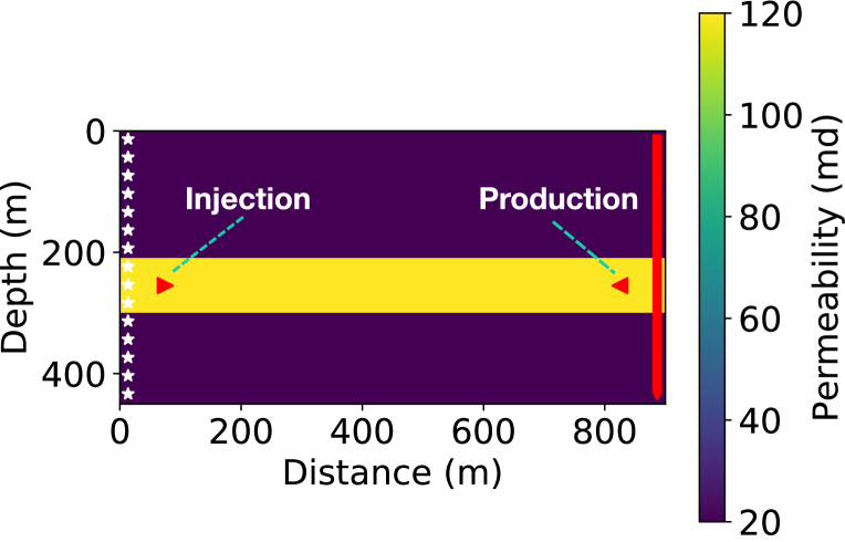
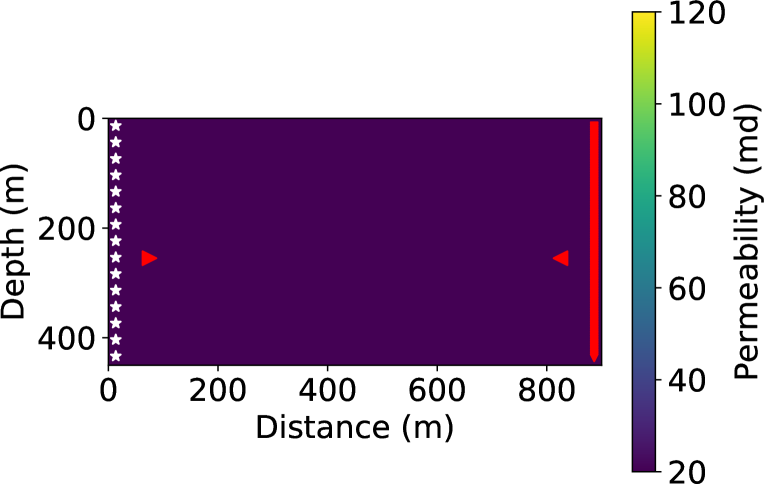
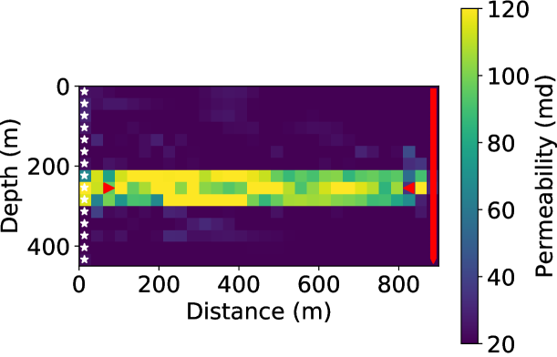
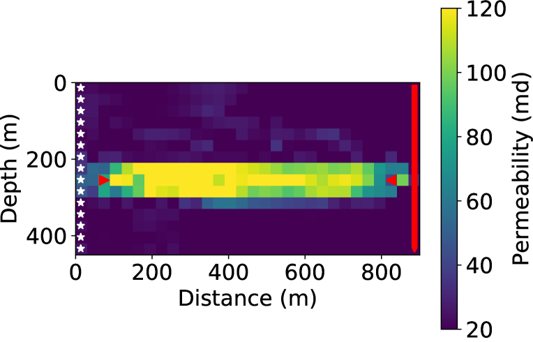
The dimension of the permeability models is m, with 15 cells in the depth direction, 30 cells in the horizontal direction. Each cell is a m block. In the true model, the background permeability is 20 millidarcy (md), while there is a high-permeability layer of 120 md in the middle, as shown in Fig. 2. In the initial model, the permeability in the whole model is 20 md. Before injection, the reservoir was filled with water, whose density is 1053.0 and viscosity is 1.0 centipoise (). The injected supercritical has a density of 501.9 and a viscosity of 0.1 . The water injection rate was 0.005 and the production well produces water at a rate of 0.005 as well. The initial , , and density models before injection are of constant values, which are 3500 m/s, m/s, and 2200 kg/m3, respectively. We simulated 51 slow-time steps at intervals of 20 days, which gives 1000-day total simulation time. Eleven of the 51, including the initial state, are used for slow-time measurements.
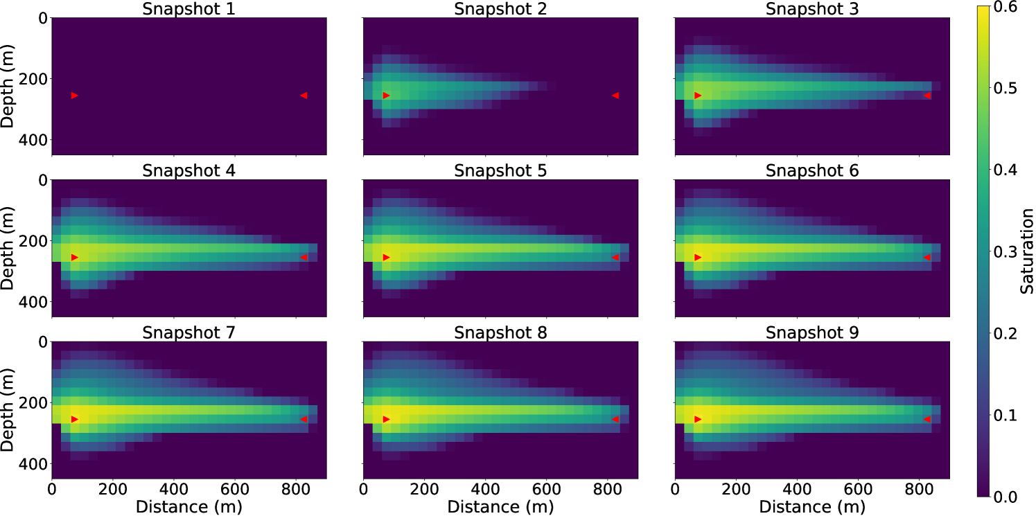
Of course the plume favors the highly permeable layer (Fig. 3) and migrate from the injection well (red triangle on the left) to the production well (red triangle on the right), while if is injected in a homogeneous reservoir, the plume expands more symmetrically towards the production well with slightly upward movement due to buoyancy.
| (a) | (b) |
|---|---|
 |
 |
We up-sampled the saturation evolution maps to a spatial grid interval of 3 , while keeping the vertical and horizontal dimensions the same. Then, the saturation maps were transformed to elastic properties, Lamé parameter , and density in our case, with the patchy saturation rock physics model.
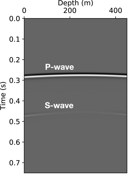
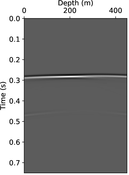
We conducted 11 crosswell seismic surveys to measure the elastic property evolutions with the slow time. In the base case, there were 15 seismic sources and 142 receivers separated by 873 . We adopted a 2-D tensile crack model [Aki \BBA Richards (\APACyear2002)] to approximate a specific radiation/sensitivity pattern of borehole sources and receivers (SI 8). The source time function was a Ricker wavelet with a dominant frequency of 50 . The seismic simulation time step was 0.00025 , and the whole simulation time was 0.75 . The shot gathers of the 8th source at the first and the eleventh survey are shown in Fig. 5. In each shot gather, the prominent events are a strong P-wave followed by a weaker S-wave. We see a slight delay in arrival time from the 1st to 11th survey, as well as slight changes in amplitude and wavefront shape in the last survey.
| (a) | (b) | (c) |
|---|---|---|
 |
 |
 |
The optimization problem was solved by the L-BFGS-B method [Byrd \BOthers. (\APACyear1995)] with a box constraint on the permeability value between 10 and 130 . L-BFGS-B is short for limited memory Broyden-Fletcher-Goldfarb-Shanno algorithm with box constraints, a standard variant of a BFGS method, which is an efficient and popular quasi-Newton algorithm for nonsmooth (both convex and nonconvex) optimization. In this work, we use the line search routine in [Moré \BBA Thuente (\APACyear1994)], which attempts to enforce the Wolfe conditions [Byrd \BOthers. (\APACyear1995)] by a sequence of polynomial interpolations.
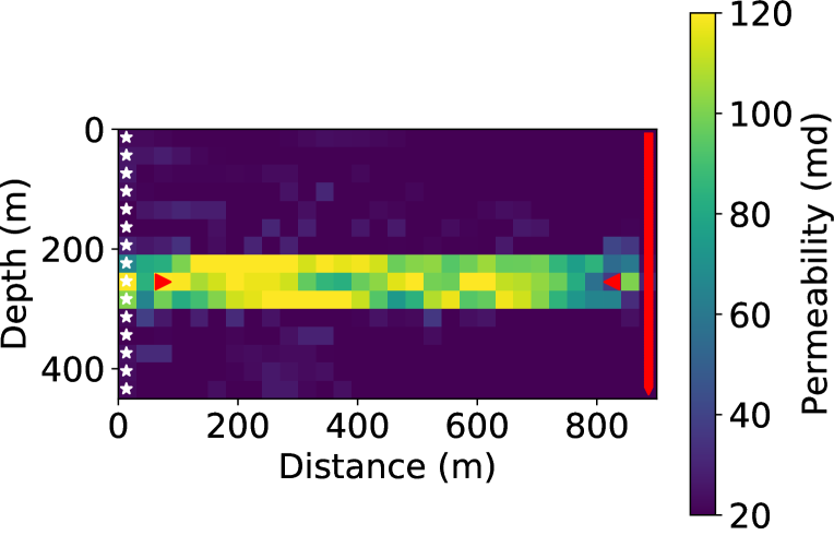
In the coupled inverted model (Fig. 8(a)), the high permeability layer was well constructed, though there are minor fluctuations in the value within the layer. To quantify the inversion accuracy, we define the mean-squared-error (MSE) measure between the true and the inverted permeability models as
| (32) |
where and are the two dimensions of discretized permeability models. We found that the MSE of the model from coupled inversion is 218.71.
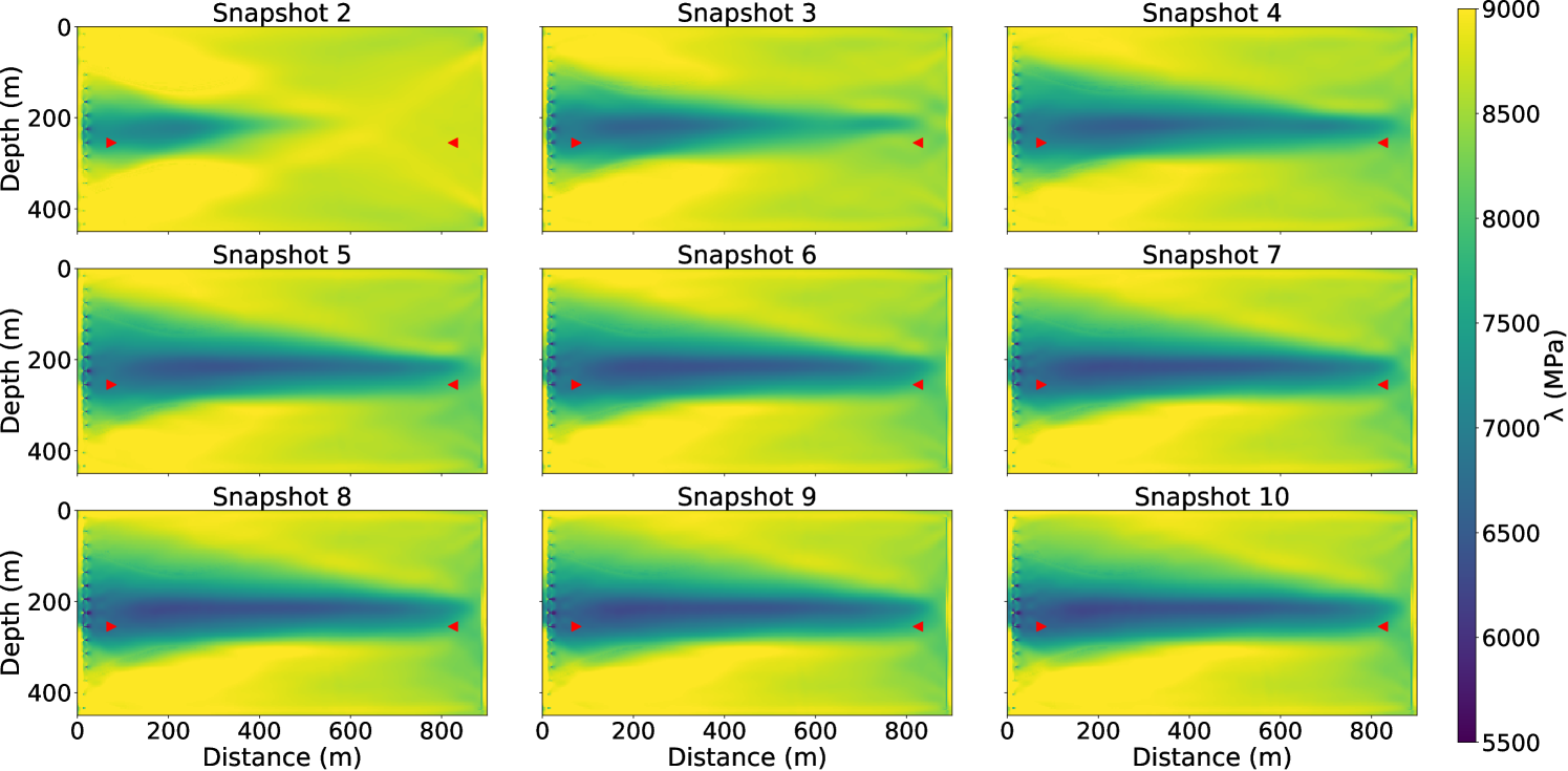
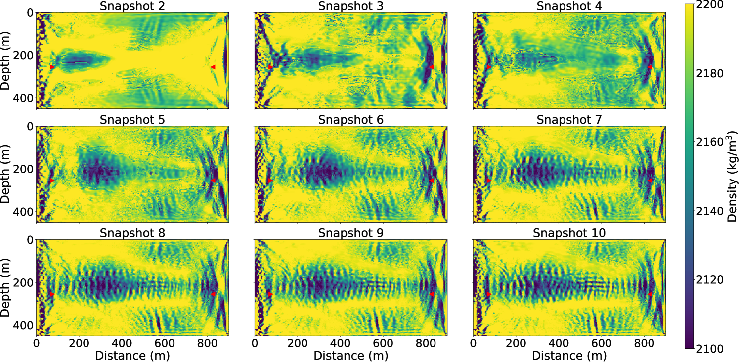
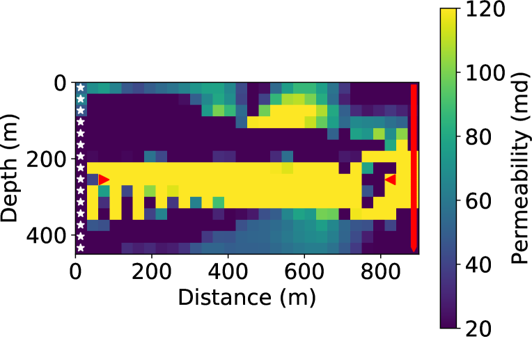
There exists a traditional choice for permeability field inversion, which we term decoupled inversion: one may separately invert for elastic properties at each snapshot using FWI, and then use the inverted elastic properties as data to fit the flow equation to reconstruct the hidden intrinsic parameter field, similar to the seismic history matching methods that we described in the introduction. This strategy has its merits of being easy to implement and helpful in quality control of each inversion component. However, seismic inversion usually carries significant inversion artifacts due to various reasons, such as limited aperture, noises in the data, and being trapped in local minima. Such seismic artifacts cannot be predicted by flow physics, and thus would lead to artifacts in the inverted intrinsic parameters in the decoupled inversion. In the coupled inversion, the flow physics PDE plays the role of spatial-temporal model regularization, which gets rid of the intermediate step in the decoupled inversion where seismic inversion artifacts accumulate. From another perspective, the coupling reduces independent elastic parameters from multiple surveys to the intrinsic parameters that do not change with time. The dimension reduction and inversion in the latent space (the space of intrinsic parameters) contribute to the reduction of artifacts. We demonstrate this issue using the same settings as the base case (11 surveys, all sources). Fig. 6 shows the inverted values for the first Lamé parameter from survey 2 to 10. Although we observe that the general shape of plume is reconstructed, artifacts due to limited aperture and strong artifacts at source locations exist. Fig. 7 shows the inverted density models from survey 2 to 10, which are corrupted by strong artifacts. This phenomenon is well-known in FWI as the phase information in the data is not sensitive to density.
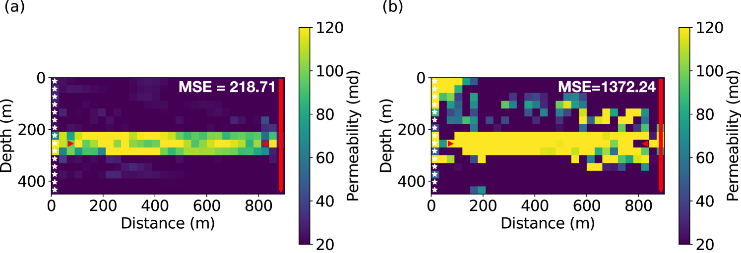
We then fitted the flow equation using -norm using the inverted Lamé values as the data. Since we attempted to obtain the best decoupled inversion result for comparison, we did not use the inverted density models due to the prevalent strong artifacts. To reduce the effects of artifacts at the seismic source and receiver locations, we excluded the left most and right most parts that include the sources and receivers for inversion, and obtained the result shown in Fig. 8(b). Compared to the model from coupled inversion (Fig. 8(a)), the permeability model from decoupled inversion is heavily contaminated with artifacts, although we can still identify the highly permeable layer. This model provides misleading information and would be harder to interpret. Also, the inverted model has a much larger MSE (1372.24) than the base case (). This experiment demonstrates the advantage and necessity of performing the coupled inversion.
| (a) |
 |
| (b) |
 |
| (c) | (d) |
|---|---|
 |
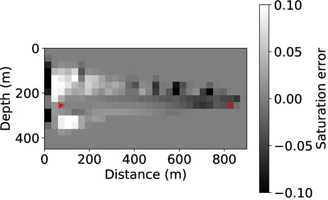 |
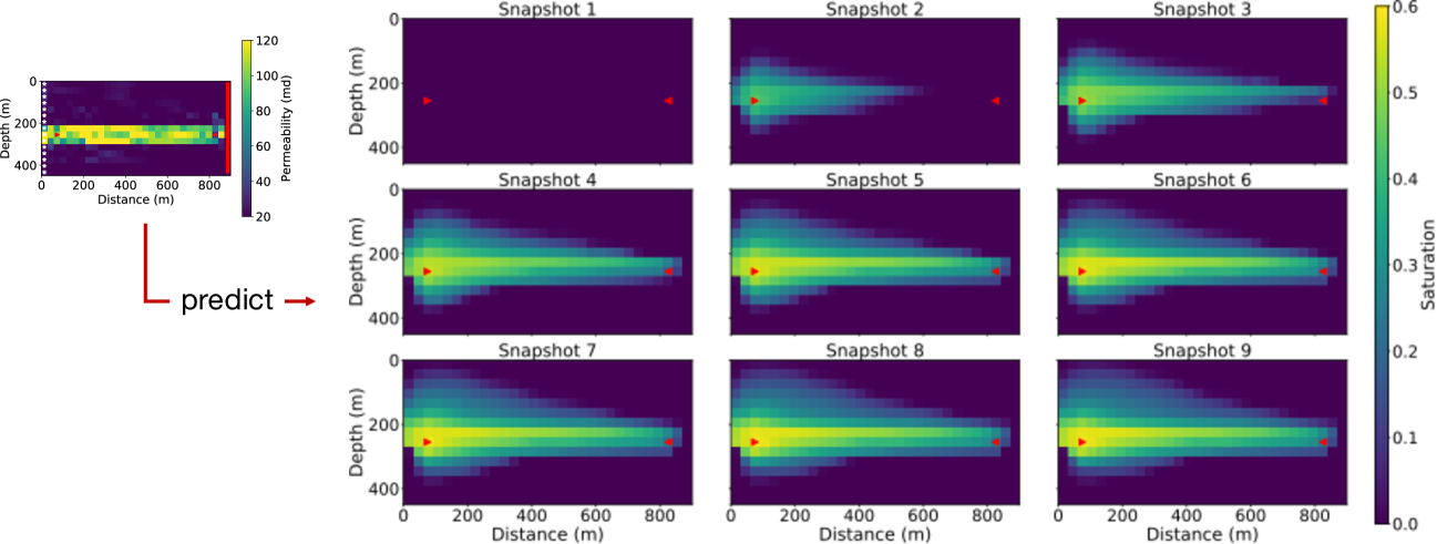
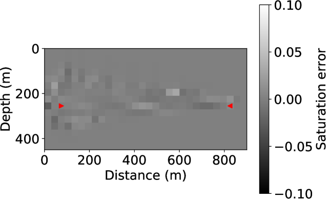
The inverted intrinsic properties can be used to predict flow behavior and also help reservoir management and optimization. With the inverted models from both the coupled and decoupled inversion strategy, we perform forward simulations of the flow and convert saturation maps to P-wave velocity maps. Fig 9(a) shows the predicted P-wave velocity evolution in slow time with the coupled inversion result, while Fig 9(b) shows the snapshots with the decoupled inversion result. The former one yields better predictions that are closer to the ground truth (Fig. 3) while the latter one leads to erroneous predictions with strong artifacts. Fig. 9(c) and (d) show that the error between the true saturation and the prediction from the decoupled inversion result is much larger than that of the coupled inversion. To further illustrate our point, we conducted forward simulations with the predicted elastic models, and compute the sum of the misfit between the predicted data and the observed data at each snapshot. The data misfit is 0.3097 for the coupled inversion, while it is 181.6226 for the decoupled inversion, which indicates that our coupled inversion can fit the data much better than the decoupled strategy.
4.2 FWI and Eikonal Equation Inversion
Full waveforms contain much more information than mere traveltime. As a result, FWI can produce results of much higher resolution than traveltime-based tomography methods such as the ray tomography. In this section, we compare the effects of using waveform data with first-arrival time only on the coupled inversion. Instead of using the traditional ray-tomography, we cast the first-arrival traveltime inversion as a PDE-constrained inversion as well using the Eikonal equation [Aki \BBA Richards (\APACyear2002)], so that we can apply our intrusive automatic differentiation (IAD) technique to this inversion problem. This formulation also reduces the error from ray-tracing, allowing a better comparison with FWI. In the synthetic tests, we assume that the Eikonal equation can accurately predict the first-arrival time. However, we should keep it in mind that the conventional ray-tomography and the Eikonal tomography are based upon the high-frequency approximation of wave propagation [Yilmaz (\APACyear2001)]; thus, there are additional errors from this inaccurate assumption in physical models. Also, there may be errors from first-arrival picking when dealing with field data.
The Eikonal equation is given by
| (33) | ||||
where is the first arrival time at location for a wave front starting at the source location , computed with the velocity field . We solve the Eikonal equation (33) using the fast sweeping method [Zhao (\APACyear2005)], which solves a system of discrete nonlinear equations at interior grid points by applying a sequence of Gauss-Seidel iterations:
where , , , and is the grid spacing.
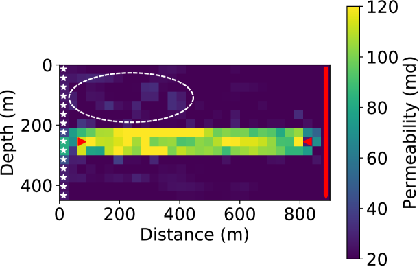
We conducted the inversion using the IAD technique, where the numerical solver and its automatic differentiation rule are implemented using a custom operator. Fig. 10 shows a comparison of the coupled inversion using the Eikonal equation and FWI. We see that the Eikonal result has stronger artifacts in the white circled area, although the two results are comparable. Table 3 summarizes a further comparison between these two methods. The result associated with FWI is much more accurate, especially when the number of sources is small, suggesting that the information beyond the first-arrival time in seismic waveforms is helpful to calibrate permeability more accurately. This is important for monitoring projects using sparsely distributed sources and receivers.
| (a) | (b) |
|---|---|
 |
 |
| 15 sources | 3 sources | 1 source | |
| FWI | 218.71 | 245.94 | 294.60 |
| Eikonal | 271.59 | 415.74 | 479.78 |
4.3 Inversion of Rock Physics Parameters
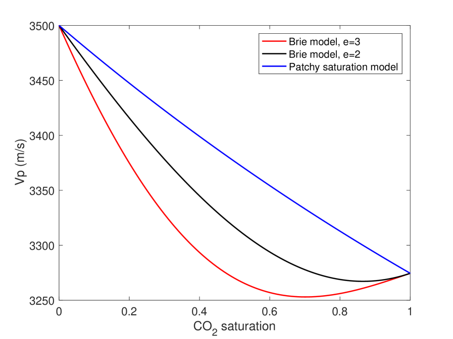
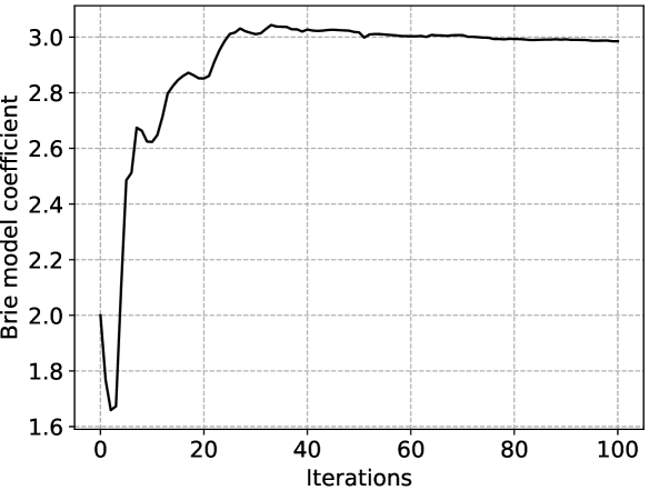
The rock physics model is a type of closure relationship that is sometimes empirical. We want to examine whether our method can also provide insight on calibration or discovery of such relationships. Therefore, we switched the rock physics model from the patchy saturation model to Gassmann’s model with Brie’s fluid mixture equation. The patchy saturation model is the upper bound of responses of elastic properties to fluid substitution. The Brie model introduced in SI 1.2.2, on the other hand, can approximate a wide range of rock physics models parameterized with the coefficient . We plot the P-wave velocity of rocks against the saturation of with the same parameters in previous numerical experiments. As is shown in Fig. (11), drops first and then increases as the saturation of increases in the Brie model, and as the coefficient decreases, the curve gradually approximates the upper bound, a straight-line predicted by the patchy saturation model.
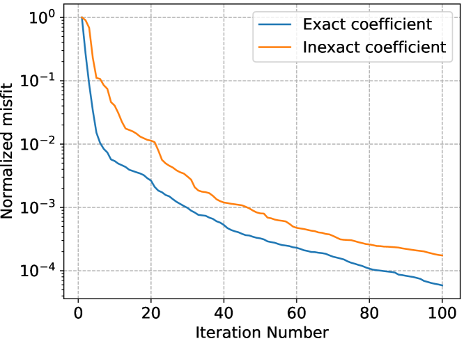
In the inversion experiments, the true rock physics model was assumed to be the Brie model with . We first used the exact rock physics model and Fig. 12(a) shows the inversion result, which has comparable accuracy as that from the patchy saturation model, with a low MSE equals 250.64. This result relies on the accurate assumption of rock physics models. However, if we have little information about the true rock physics model and wrongly assume that , Fig. 12(b) shows the inverted result that has much stronger artifacts and much higher MSE (2098.02). To mitigate such a common problem, we invert for the Brie’s coefficient and permeability simultaneously. Thanks to the automatic differentiation capability of the framework, the gradient of the misfit function with respect to can be easily obtained. The initial guess of was also 2 as the previous experiment. Considering the range of value of the coefficient is different from that of the permeability, we scaled up the value of parameter by 30 and divided it by 30 before feeding it to the rock physics equations. Fig. 12(c) shows the inverted permeability with updated simultaneously, which is more accurate (MSE = 320.04) than the previous case without updating. We show the inversion history of the coefficient in Fig. 12(d), which quickly converges to the true after around 40 iterations. The initial drop of the value at the beginning several iterations are probably caused by the fact that the L-BFGS-B optimizer essentially acts as a gradient-descent at the beginning, which cannot handle the scaling of different parameters of different physical meanings well. This phenomenon was severe without the scaling trick that we just mentioned. In Fig. 12(e), we observe good convergence in data misfit of the simultaneous inversion. This promising result not only presents the multi-parameter inversion capability enabled by the automatic differentiable computing but also emphasizes that the simultaneous inversion can yield more accurate inversion results and provide insights on empirical relationships in practice.
| (a) | (b) |
|---|---|
 |
 |
| (c) | (d) |
|---|---|
 |
 |
| (e) |
 |
4.4 A 2-D Stream Channel Model
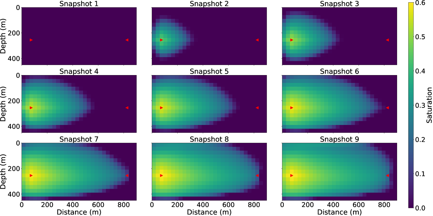
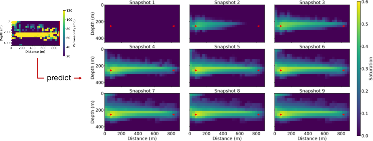
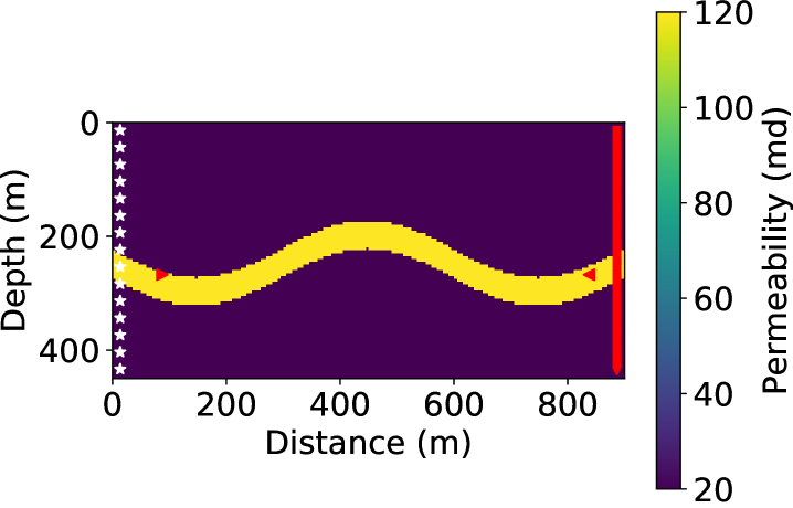
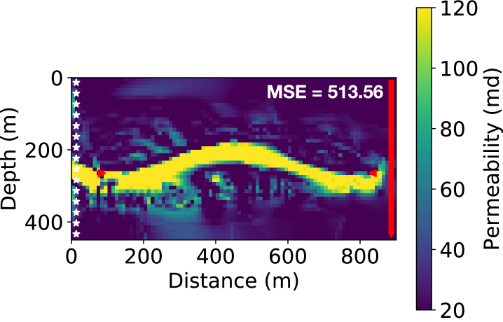
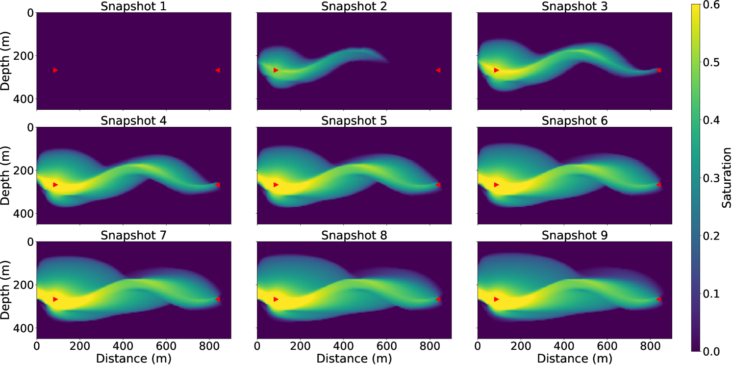
In addition to the 3-layer model of horizontal layers, we also tested the coupled inversion for a stream channel model shown in Fig. 13(a), where the channel has a permeability of 120 md while the background is 20 md. This example can represent a vertical slice between vertical wells or a horizontal slice between horizontal wells.
This model has the same dimension as the 3-layer model, but has a smaller grid size of 5 m in both the vertical and horizontal directions, hence the model is parameterized by cells. We used this discretized model to create synthetic observed data. The synthetic saturation evolution maps for this channel model is shown in Fig. 14 for nine snapshots in slow-time. For the inversion, we increase the grid size to 10 m yielding a grid of cells. The initial model is a homogeneous model of permeability of 20 md as previous experiments. Fig. 13(b) show the inversion result with data from 11 surveys after 100 iterations, which is the same all-at-once strategy as previous experiments. The 2-D channel is well reconstructed, meaning that our algorithm can also resolve complex 2-D structures with denser parameterization. The artifacts seen can be reduced by geological parameterization [Landa \BOthers. (\APACyear1997)], or regularization methods [Aster \BOthers. (\APACyear2013), D. Li \BBA Harris (\APACyear2018)].
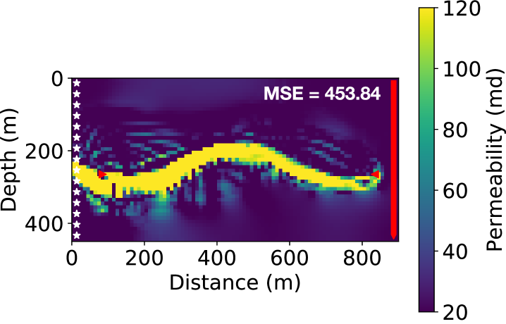
In real-world operations, it would be rare to wait and begin data analysis after completion of all surveys. Instead, it is a more practical strategy to perform continuous inversion along with new data from continuing surveys. In other words, at the end of survey , we formulate an optimization/inversion problem with all available data so far and use the model from the previous stage of inversion as the initial model. We also tested the new strategy in this case. After a continuous inversion of only 6 surveys, we did not observe further improvement on the inversion result and report the inverted permeability model in Fig. 13(c), which seems to have fewer artifacts and lower MSE than that from the all-at-once strategy. Instead of inverting for all parameters at the same time, the continuous inversion strategy breaks the original problem into progressive bits, and it is easier to reconstruct the permeability field incrementally. Also, an accurate estimation of the flow properties at an early stage largely determines the accuracy of the following inversions due to the underlying physics model.
| (a) | (b) |
|---|---|
 |
 |
| (c) |
 |
Remark.
In a more realistic setting, the permeability within the channel may also be spatially varying instead of having a constant value. As an additional example, we summarize the inversion results for this scenario in the supporting information (SI 7). We show that our method is also effective for calibrating space-varying permeability within the channels.
5 Discussion & Conclusions
We have presented a novel approach for estimating intrinsic rock parameters (e.g., permeability) from time-lapse full-waveform inversion of geophysical data (e.g., seismic data). We demonstrated that solving an inverse problem constrained by coupled physical systems is superior to a decoupled inversion in terms of accuracy. Additionally, we found that the full waveform data carry richer information than first-arrival travel time data for calibrating hydrological properties. Also, the method is effective in inverting an empirical rock physics model while estimating the subsurface permeability map at the same time.
To solve the coupled inverse problem, we proposed the intrusive automatic differentiation (IAD) method. This strategy combines different levels of control over gradient computation schemes in an intrusive way to an automatic differentiation computational workflow: custom PDE operators for time step marching in solving the flow equations, built-in differentiable operators from TensorFlow for the rock physics models, and the discrete adjoint method for wave physics. With this strategy, we can fully exploit the power of modern machine learning platforms, and also make computations more efficient when necessary with algebraic multi-grid fast solvers, the Newton-Raphson method, an optimized GPU-accelerated FWI module, and in general various memory-saving techniques. The coupled inversion technique—intrusive automatic differentiation (IAD)—as well as the software we developed, can be applied to other joint/coupled inversion problems as well. We hope the tools can stimulate further inverse modeling applications.
Some work remains to be done for inverse modeling with coupled PDE systems and hidden dynamics of subsurface flow. First, the rock physics conversion requires accurate reference elastic properties, on which elastic properties are based and altered by fluid substitution. Inaccurate reference properties may lead to non-physical elastic properties at subsequent survey times, making it difficult to fit the physics-based PDEs. Thus, we strongly advise one to estimate the reference properties as accurately as possible before subsequent time-lapse inversion. Also, the so-called “e factor” may for example depend on lithology. Second, seismic wave attenuation effects may be significant in flow-related problems. We can incorporate viscoelastic effects in wave physics modeling and expand elastic properties to anelastic properties, thus exploiting more wave physics behavior for flow inversion problems. Third, the gradient computation within the framework of automatic differentiation, which ADCME is based on, requires storing intermediate results for gradient back-propagation. In some situations, this will place excessive pressure on memory requirements. Checkpointing schemes can be used to alleviate this problem but require additional effort to implement. Finally, we must exercise care when interpreting the calibrated permeability or other hidden intrinsic parameters. If the flow has not reached certain areas throughout the slow time, the objective function has no sensitivity to flow parameters in those areas. Due to the characteristics of the L-BFGS-B optimizer, there will be no update in places where the gradient is always zero. Therefore, one may want to examine the flow simulation with the inverted model to determine the areas valid for further analysis. One can also employ regularization methods as well as the multi-scale inversion strategy (i.e., to invert from low frequency to high frequency, from coarse parameterization to fine parameterization) to increase the robustness of inversion.
These questions form a promising line of future research. While our extensive numerical investigation shows the applicability and effectiveness of this novel approach, answering these questions is critical for deeper understanding and more practical applications.
-
•
First, one such focused area we are pursuing is the investigation of the robustness of our coupled physics and intrusive automatic differentiation approach to sparse datasets, that is, sparsity in space and slow-time. This problem is essential when continuous subsurface monitoring strategies are needed, and full datasets are expensive to record at each slow-time step.
-
•
Second, the inversion problem is more challenging in the presence of fractures. In this scenario, we need a reservoir simulator to handle the fractures, which requires a significant finer or an adaptive grid, and conduct automatic differentiation through this simulator. The resolution of hydrological properties that we reconstruct from seismic data in the presence of fractures also remains to be studied.
-
•
Third, the rock physics relationship can be heterogeneous in space. In our examples, we assume a homogeneous relationship as most coupled inversion practices, although we demonstrate that it is possible to calibrate the scalar parameter. In a future research direction, it is well worth considering inverting for a spatially variable rock physics parameter. This is again a multi-parameter inversion problem, where proper scaling may be critical, and alternate inversion of intrinsic parameters and rock physics parameters may also be necessary. The calibration of such a rock physics model with spatial variability can also be helpful for interpretation tasks.
-
•
Finally, we note that our approach, demonstrated here in 2-D, is fully expandable to more realistic settings in 3-D surface seismic, VSP seismic, and small-scale crosswell seismic surveys. Different geometries have different advantages and weaknesses. For example, the surface seismic surveys can monitor a large-scale reservoir, but the resolution is relatively low due to the limited high-frequency components in the data (up to tens of Hertz), and limited sampling of low-wavenumber components. On the contrary, small-scale crosswell surveys can generate data of frequency up to several thousand Hertz, sensitive to small-scale flow patterns, leading to a high-resolution delineation of the subsurface parameters, but it may not be able to monitor the whole reservoir. Practitioners can choose which geometry to use according to the problem at hand.
Acknowledgements.
The authors thank Biondo Biondi, Tapan Mukerji, and Gerald Mavko for many helpful discussions. Kailai Xu is supported by the Applied Mathematics Program within the Department of Energy (DOE) Office of Advanced Scientific Computing Research (ASCR), through the Collaboratory on Mathematics and Physics-Informed Learning Machines for Multiscale and Multiphysics Problems Research Center (DE-SC0019453). The source code of this project can be found at https://github.com/lidongzh/FwiFlow.jl, which generates all synthetic data used in this paper. We greatly appreciate the constructive and detailed comments and suggestions from associate editor Dr. Huisman and three anonymous reviewers.References
- Abadi \BOthers. (\APACyear2016) \APACinsertmetastarabadi2016tensorflow{APACrefauthors}Abadi, M.\BCBT \BOthersPeriod. \APACrefYearMonthDay2016. \BBOQ\APACrefatitleTensorflow: A system for large-scale machine learning Tensorflow: A system for large-scale machine learning.\BBCQ \BIn \APACrefbtitle12th USENIX Symposium on Operating Systems Design and Implementation (OSDI’16) 12th USENIX symposium on operating systems design and implementation (OSDI’16) (\BPG 265-283). \PrintBackRefs\CurrentBib
- Aki \BBA Richards (\APACyear2002) \APACinsertmetastaraki2002quantitative{APACrefauthors}Aki, K.\BCBT \BBA Richards, P\BPBIG. \APACrefYear2002. \APACrefbtitleQuantitative seismology Quantitative seismology (\PrintOrdinalSecond \BEd). \APACaddressPublisherUniversity Science Books. \PrintBackRefs\CurrentBib
- Anderson \BOthers. (\APACyear2012) \APACinsertmetastaranderson2012time{APACrefauthors}Anderson, J\BPBIE., Tan, L.\BCBL \BBA Wang, D. \APACrefYearMonthDay2012. \BBOQ\APACrefatitleTime-reversal checkpointing methods for RTM and FWI Time-reversal checkpointing methods for RTM and FWI.\BBCQ \APACjournalVolNumPagesGeophysics774S93–S103. \PrintBackRefs\CurrentBib
- Archie \BOthers. (\APACyear1942) \APACinsertmetastararchie1942electrical{APACrefauthors}Archie, G\BPBIE.\BCBT \BOthersPeriod. \APACrefYearMonthDay1942. \BBOQ\APACrefatitleThe electrical resistivity log as an aid in determining some reservoir characteristics The electrical resistivity log as an aid in determining some reservoir characteristics.\BBCQ \APACjournalVolNumPagesTransactions of the AIME1460154–62. \PrintBackRefs\CurrentBib
- Aster \BOthers. (\APACyear2013) \APACinsertmetastarAster201393{APACrefauthors}Aster, R\BPBIC., Borchers, B.\BCBL \BBA Thurber, C\BPBIH. \APACrefYearMonthDay2013. \BBOQ\APACrefatitleChapter Four - Tikhonov Regularization Chapter four - Tikhonov regularization.\BBCQ \BIn R\BPBIC. Aster, B. Borchers\BCBL \BBA C\BPBIH. Thurber (\BEDS), \APACrefbtitleParameter Estimation and Inverse Problems (Second Edition) Parameter estimation and inverse problems (second edition) (\PrintOrdinalSecond Edition \BEd, \BPG 93 - 127). \APACaddressPublisherBostonAcademic Press. {APACrefURL} http://www.sciencedirect.com/science/article/pii/B9780123850485000045 {APACrefDOI} http://dx.doi.org/10.1016/B978-0-12-385048-5.00004-5 \PrintBackRefs\CurrentBib
- Beaujean \BOthers. (\APACyear2014) \APACinsertmetastarbeaujean2014calibration{APACrefauthors}Beaujean, J., Nguyen, F., Kemna, A., Antonsson, A.\BCBL \BBA Engesgaard, P. \APACrefYearMonthDay2014. \BBOQ\APACrefatitleCalibration of seawater intrusion models: Inverse parameter estimation using surface electrical resistivity tomography and borehole data Calibration of seawater intrusion models: Inverse parameter estimation using surface electrical resistivity tomography and borehole data.\BBCQ \APACjournalVolNumPagesWater Resources Research5086828–6849. \PrintBackRefs\CurrentBib
- Brie \BOthers. (\APACyear1995) \APACinsertmetastarbrie1995shear{APACrefauthors}Brie, A., Pampuri, F., Marsala, A., Meazza, O.\BCBL \BOthersPeriod. \APACrefYearMonthDay1995. \BBOQ\APACrefatitleShear sonic interpretation in gas-bearing sands Shear sonic interpretation in gas-bearing sands.\BBCQ \BIn \APACrefbtitleSPE Annual Technical Conference and Exhibition. Spe annual technical conference and exhibition. \PrintBackRefs\CurrentBib
- Brooks \BBA Corey (\APACyear1964) \APACinsertmetastarbrooks1964hydrau{APACrefauthors}Brooks, R.\BCBT \BBA Corey, T. \APACrefYearMonthDay1964. \BBOQ\APACrefatitleHYDRAU uc properties of porous media Hydrau uc properties of porous media.\BBCQ \APACjournalVolNumPagesHydrology Papers, Colorado State University2437. \PrintBackRefs\CurrentBib
- Byrd \BOthers. (\APACyear1995) \APACinsertmetastarbyrd1995limited{APACrefauthors}Byrd, R\BPBIH., Lu, P., Nocedal, J.\BCBL \BBA Zhu, C. \APACrefYearMonthDay1995. \BBOQ\APACrefatitleA limited memory algorithm for bound constrained optimization A limited memory algorithm for bound constrained optimization.\BBCQ \APACjournalVolNumPagesSIAM Journal on Scientific Computing1651190–1208. \PrintBackRefs\CurrentBib
- Carter \BOthers. (\APACyear1974) \APACinsertmetastarcarter1974performance{APACrefauthors}Carter, R., Kemp Jr, L., Pierce, A., Williams, D.\BCBL \BOthersPeriod. \APACrefYearMonthDay1974. \BBOQ\APACrefatitlePerformance matching with constraints Performance matching with constraints.\BBCQ \APACjournalVolNumPagesSociety of Petroleum Engineers Journal1402187–196. \PrintBackRefs\CurrentBib
- Chavent \BOthers. (\APACyear1975) \APACinsertmetastarchavent1975history{APACrefauthors}Chavent, G., Dupuy, M., Lemmonier, P.\BCBL \BOthersPeriod. \APACrefYearMonthDay1975. \BBOQ\APACrefatitleHistory matching by use of optimal theory History matching by use of optimal theory.\BBCQ \APACjournalVolNumPagesSociety of Petroleum Engineers Journal150174–86. \PrintBackRefs\CurrentBib
- Chen \BOthers. (\APACyear1974) \APACinsertmetastarchen1974new{APACrefauthors}Chen, W\BPBIH., Gavalas, G\BPBIR., Seinfeld, J\BPBIH.\BCBL \BBA Wasserman, M\BPBIL. \APACrefYearMonthDay1974. \BBOQ\APACrefatitleA new algorithm for automatic history matching A new algorithm for automatic history matching.\BBCQ \APACjournalVolNumPagesSociety of Petroleum Engineers Journal146593–608. \PrintBackRefs\CurrentBib
- Copty \BOthers. (\APACyear1993) \APACinsertmetastarcopty1993geophysical{APACrefauthors}Copty, N., Rubin, Y.\BCBL \BBA Mavko, G. \APACrefYearMonthDay1993. \BBOQ\APACrefatitleGeophysical-hydrological identification of field permeabilities through Bayesian updating Geophysical-hydrological identification of field permeabilities through bayesian updating.\BBCQ \APACjournalVolNumPagesWater Resources Research2982813–2825. \PrintBackRefs\CurrentBib
- Corey \BOthers. (\APACyear1954) \APACinsertmetastarcorey1954interrelation{APACrefauthors}Corey, A\BPBIT.\BCBT \BOthersPeriod. \APACrefYearMonthDay1954. \BBOQ\APACrefatitleThe interrelation between gas and oil relative permeabilities The interrelation between gas and oil relative permeabilities.\BBCQ \APACjournalVolNumPagesProducers monthly19138–41. \PrintBackRefs\CurrentBib
- Day-Lewis \BBA Lane Jr (\APACyear2004) \APACinsertmetastarday2004assessing{APACrefauthors}Day-Lewis, F.\BCBT \BBA Lane Jr, J. \APACrefYearMonthDay2004. \BBOQ\APACrefatitleAssessing the resolution-dependent utility of tomograms for geostatistics Assessing the resolution-dependent utility of tomograms for geostatistics.\BBCQ \APACjournalVolNumPagesGeophysical Research Letters317. \PrintBackRefs\CurrentBib
- Emerick \BOthers. (\APACyear2007) \APACinsertmetastaremerick2007history{APACrefauthors}Emerick, A\BPBIA., Moraes, R., Rodrigues, J.\BCBL \BOthersPeriod. \APACrefYearMonthDay2007. \BBOQ\APACrefatitleHistory matching 4D seismic data with efficient gradient based methods History matching 4d seismic data with efficient gradient based methods.\BBCQ \BIn \APACrefbtitleEUROPEC/EAGE Conference and Exhibition. Europec/eage conference and exhibition. \PrintBackRefs\CurrentBib
- Gueting \BOthers. (\APACyear2015) \APACinsertmetastargueting2015imaging{APACrefauthors}Gueting, N., Klotzsche, A., van der Kruk, J., Vanderborght, J., Vereecken, H.\BCBL \BBA Englert, A. \APACrefYearMonthDay2015. \BBOQ\APACrefatitleImaging and characterization of facies heterogeneity in an alluvial aquifer using GPR full-waveform inversion and cone penetration tests Imaging and characterization of facies heterogeneity in an alluvial aquifer using gpr full-waveform inversion and cone penetration tests.\BBCQ \APACjournalVolNumPagesJournal of hydrology524680–695. \PrintBackRefs\CurrentBib
- Gueting \BOthers. (\APACyear2017) \APACinsertmetastargueting2017high{APACrefauthors}Gueting, N., Vienken, T., Klotzsche, A., Van Der Kruk, J., Vanderborght, J., Caers, J.\BDBLEnglert, A. \APACrefYearMonthDay2017. \BBOQ\APACrefatitleHigh resolution aquifer characterization using crosshole GPR full-waveform tomography: Comparison with direct-push and tracer test data High resolution aquifer characterization using crosshole gpr full-waveform tomography: Comparison with direct-push and tracer test data.\BBCQ \APACjournalVolNumPagesWater Resources Research53149–72. \PrintBackRefs\CurrentBib
- Hinnell \BOthers. (\APACyear2010) \APACinsertmetastarhinnell2010improved{APACrefauthors}Hinnell, A., Ferré, T., Vrugt, J., Huisman, J., Moysey, S., Rings, J.\BCBL \BBA Kowalsky, M. \APACrefYearMonthDay2010. \BBOQ\APACrefatitleImproved extraction of hydrologic information from geophysical data through coupled hydrogeophysical inversion Improved extraction of hydrologic information from geophysical data through coupled hydrogeophysical inversion.\BBCQ \APACjournalVolNumPagesWater resources research464. \PrintBackRefs\CurrentBib
- Huang \BOthers. (\APACyear1998) \APACinsertmetastarhuang1998improving{APACrefauthors}Huang, X., Meister, L.\BCBL \BBA Workman, R. \APACrefYearMonthDay1998. \BBOQ\APACrefatitleImproving production history matching using time-lapse seismic data Improving production history matching using time-lapse seismic data.\BBCQ \APACjournalVolNumPagesThe Leading Edge17101430–1433. \PrintBackRefs\CurrentBib
- Huisman \BOthers. (\APACyear2010) \APACinsertmetastarhuisman2010hydraulic{APACrefauthors}Huisman, J., Rings, J., Vrugt, J., Sorg, J.\BCBL \BBA Vereecken, H. \APACrefYearMonthDay2010. \BBOQ\APACrefatitleHydraulic properties of a model dike from coupled Bayesian and multi-criteria hydrogeophysical inversion Hydraulic properties of a model dike from coupled bayesian and multi-criteria hydrogeophysical inversion.\BBCQ \APACjournalVolNumPagesJournal of Hydrology3801-262–73. \PrintBackRefs\CurrentBib
- Irving \BBA Singha (\APACyear2010) \APACinsertmetastarirving2010stochastic{APACrefauthors}Irving, J.\BCBT \BBA Singha, K. \APACrefYearMonthDay2010. \BBOQ\APACrefatitleStochastic inversion of tracer test and electrical geophysical data to estimate hydraulic conductivities Stochastic inversion of tracer test and electrical geophysical data to estimate hydraulic conductivities.\BBCQ \APACjournalVolNumPagesWater Resources Research4611. \PrintBackRefs\CurrentBib
- Jardani \BOthers. (\APACyear2013) \APACinsertmetastarjardani2013stochastic{APACrefauthors}Jardani, A., Revil, A.\BCBL \BBA Dupont, J\BHBIP. \APACrefYearMonthDay2013. \BBOQ\APACrefatitleStochastic joint inversion of hydrogeophysical data for salt tracer test monitoring and hydraulic conductivity imaging Stochastic joint inversion of hydrogeophysical data for salt tracer test monitoring and hydraulic conductivity imaging.\BBCQ \APACjournalVolNumPagesAdvances in water resources5262–77. \PrintBackRefs\CurrentBib
- Keskinen \BOthers. (\APACyear2017) \APACinsertmetastarkeskinen2017full{APACrefauthors}Keskinen, J., Klotzsche, A., Looms, M\BPBIC., Moreau, J., van der Kruk, J., Holliger, K.\BDBLNielsen, L. \APACrefYearMonthDay2017. \BBOQ\APACrefatitleFull-waveform inversion of crosshole GPR data: Implications for porosity estimation in chalk Full-waveform inversion of crosshole gpr data: Implications for porosity estimation in chalk.\BBCQ \APACjournalVolNumPagesJournal of Applied Geophysics140102–116. \PrintBackRefs\CurrentBib
- Klotzsche \BOthers. (\APACyear2014) \APACinsertmetastarklotzsche2014detection{APACrefauthors}Klotzsche, A., van der Kruk, J., Bradford, J.\BCBL \BBA Vereecken, H. \APACrefYearMonthDay2014. \BBOQ\APACrefatitleDetection of spatially limited high-porosity layers using crosshole GPR signal analysis and full-waveform inversion Detection of spatially limited high-porosity layers using crosshole gpr signal analysis and full-waveform inversion.\BBCQ \APACjournalVolNumPagesWater Resources Research5086966–6985. \PrintBackRefs\CurrentBib
- Klotzsche \BOthers. (\APACyear2012) \APACinsertmetastarklotzsche2012crosshole{APACrefauthors}Klotzsche, A., van der Kruk, J., Meles, G.\BCBL \BBA Vereecken, H. \APACrefYearMonthDay2012. \BBOQ\APACrefatitleCrosshole GPR full-waveform inversion of waveguides acting as preferential flow paths within aquifer systems Crosshole gpr full-waveform inversion of waveguides acting as preferential flow paths within aquifer systems.\BBCQ \APACjournalVolNumPagesGeophysics774H57–H62. \PrintBackRefs\CurrentBib
- Kowalsky \BOthers. (\APACyear2005) \APACinsertmetastarkowalsky2005estimation{APACrefauthors}Kowalsky, M\BPBIB., Finsterle, S., Peterson, J., Hubbard, S., Rubin, Y., Majer, E.\BDBLGee, G. \APACrefYearMonthDay2005. \BBOQ\APACrefatitleEstimation of field-scale soil hydraulic and dielectric parameters through joint inversion of GPR and hydrological data Estimation of field-scale soil hydraulic and dielectric parameters through joint inversion of GPR and hydrological data.\BBCQ \APACjournalVolNumPagesWater Resources Research4111. \PrintBackRefs\CurrentBib
- Kowalsky \BOthers. (\APACyear2004) \APACinsertmetastarkowalsky2004estimating{APACrefauthors}Kowalsky, M\BPBIB., Finsterle, S.\BCBL \BBA Rubin, Y. \APACrefYearMonthDay2004. \BBOQ\APACrefatitleEstimating flow parameter distributions using ground-penetrating radar and hydrological measurements during transient flow in the vadose zone Estimating flow parameter distributions using ground-penetrating radar and hydrological measurements during transient flow in the vadose zone.\BBCQ \APACjournalVolNumPagesAdvances in Water Resources276583–599. \PrintBackRefs\CurrentBib
- Landa \BOthers. (\APACyear1997) \APACinsertmetastarlanda1997procedure{APACrefauthors}Landa, J\BPBIL., Horne, R\BPBIN.\BCBL \BOthersPeriod. \APACrefYearMonthDay1997. \BBOQ\APACrefatitleA procedure to integrate well test data, reservoir performance history and 4-D seismic information into a reservoir description A procedure to integrate well test data, reservoir performance history and 4-d seismic information into a reservoir description.\BBCQ \BIn \APACrefbtitleSPE Annual Technical Conference and Exhibition. Spe annual technical conference and exhibition. \PrintBackRefs\CurrentBib
- D. Li \BBA Harris (\APACyear2018) \APACinsertmetastarli2018full{APACrefauthors}Li, D.\BCBT \BBA Harris, J\BPBIM. \APACrefYearMonthDay2018. \BBOQ\APACrefatitleFull waveform inversion with nonlocal similarity and model-derivative domain adaptive sparsity-promoting regularization Full waveform inversion with nonlocal similarity and model-derivative domain adaptive sparsity-promoting regularization.\BBCQ \APACjournalVolNumPagesGeophysical Journal International21531841–1864. \PrintBackRefs\CurrentBib
- R. Li \BOthers. (\APACyear2001) \APACinsertmetastarli2001history{APACrefauthors}Li, R., Reynolds, A\BPBIC., Oliver, D\BPBIS.\BCBL \BOthersPeriod. \APACrefYearMonthDay2001. \BBOQ\APACrefatitleHistory matching of three-phase flow production data History matching of three-phase flow production data.\BBCQ \BIn \APACrefbtitleSPE reservoir simulation symposium. Spe reservoir simulation symposium. \PrintBackRefs\CurrentBib
- Lie (\APACyear2019) \APACinsertmetastarlie2019introduction{APACrefauthors}Lie, K\BHBIA. \APACrefYear2019. \APACrefbtitleAn introduction to reservoir simulation using MATLAB/GNU Octave An introduction to reservoir simulation using matlab/gnu octave. \APACaddressPublisherCambridge University Press. \PrintBackRefs\CurrentBib
- Linde \BBA Doetsch (\APACyear2016) \APACinsertmetastarlinde2016joint{APACrefauthors}Linde, N.\BCBT \BBA Doetsch, J. \APACrefYearMonthDay2016. \BBOQ\APACrefatitleJoint inversion in hydrogeophysics and near-surface geophysics Joint inversion in hydrogeophysics and near-surface geophysics.\BBCQ \APACjournalVolNumPagesIntegrated imaging of the Earth: Theory and applications218119. \PrintBackRefs\CurrentBib
- Marotzke \BOthers. (\APACyear1999) \APACinsertmetastarmarotzke1999construction{APACrefauthors}Marotzke, J., Giering, R., Zhang, K\BPBIQ., Stammer, D., Hill, C.\BCBL \BBA Lee, T. \APACrefYearMonthDay1999. \BBOQ\APACrefatitleConstruction of the adjoint MIT ocean general circulation model and application to Atlantic heat transport sensitivity Construction of the adjoint mit ocean general circulation model and application to atlantic heat transport sensitivity.\BBCQ \APACjournalVolNumPagesJournal of Geophysical Research: Oceans104C1229529–29547. \PrintBackRefs\CurrentBib
- Martin \BOthers. (\APACyear2008) \APACinsertmetastarmartin2008unsplit{APACrefauthors}Martin, R., Komatitsch, D.\BCBL \BBA Ezziani, A. \APACrefYearMonthDay2008. \BBOQ\APACrefatitleAn unsplit convolutional perfectly matched layer improved at grazing incidence for seismic wave propagation in poroelastic media An unsplit convolutional perfectly matched layer improved at grazing incidence for seismic wave propagation in poroelastic media.\BBCQ \APACjournalVolNumPagesGeophysics734T51–T61. \PrintBackRefs\CurrentBib
- Mavko \BOthers. (\APACyear2009) \APACinsertmetastarmavko2009rock{APACrefauthors}Mavko, G., Mukerji, T.\BCBL \BBA Dvorkin, J. \APACrefYear2009. \APACrefbtitleThe rock physics handbook: Tools for seismic analysis of porous media The rock physics handbook: Tools for seismic analysis of porous media. \APACaddressPublisherCambridge university press. \PrintBackRefs\CurrentBib
- McLaughlin \BBA Townley (\APACyear1996) \APACinsertmetastarmclaughlin1996reassessment{APACrefauthors}McLaughlin, D.\BCBT \BBA Townley, L\BPBIR. \APACrefYearMonthDay1996. \BBOQ\APACrefatitleA reassessment of the groundwater inverse problem A reassessment of the groundwater inverse problem.\BBCQ \APACjournalVolNumPagesWater Resources Research3251131–1161. \PrintBackRefs\CurrentBib
- Moré \BBA Thuente (\APACyear1994) \APACinsertmetastarmore1994line{APACrefauthors}Moré, J\BPBIJ.\BCBT \BBA Thuente, D\BPBIJ. \APACrefYearMonthDay1994. \BBOQ\APACrefatitleLine search algorithms with guaranteed sufficient decrease Line search algorithms with guaranteed sufficient decrease.\BBCQ \APACjournalVolNumPagesACM Transactions on Mathematical Software (TOMS)203286–307. \PrintBackRefs\CurrentBib
- Mualem (\APACyear1976) \APACinsertmetastarmualem1976new{APACrefauthors}Mualem, Y. \APACrefYearMonthDay1976. \BBOQ\APACrefatitleA new model for predicting the hydraulic conductivity of unsaturated porous media A new model for predicting the hydraulic conductivity of unsaturated porous media.\BBCQ \APACjournalVolNumPagesWater resources research123513–522. \PrintBackRefs\CurrentBib
- Oliver \BBA Chen (\APACyear2011) \APACinsertmetastaroliver2011recent{APACrefauthors}Oliver, D\BPBIS.\BCBT \BBA Chen, Y. \APACrefYearMonthDay2011. \BBOQ\APACrefatitleRecent progress on reservoir history matching: a review Recent progress on reservoir history matching: a review.\BBCQ \APACjournalVolNumPagesComputational Geosciences151185–221. \PrintBackRefs\CurrentBib
- Pollock \BBA Cirpka (\APACyear2010) \APACinsertmetastarpollock2010fully{APACrefauthors}Pollock, D.\BCBT \BBA Cirpka, O\BPBIA. \APACrefYearMonthDay2010. \BBOQ\APACrefatitleFully coupled hydrogeophysical inversion of synthetic salt tracer experiments Fully coupled hydrogeophysical inversion of synthetic salt tracer experiments.\BBCQ \APACjournalVolNumPagesWater Resources Research467. \PrintBackRefs\CurrentBib
- Pollock \BBA Cirpka (\APACyear2012) \APACinsertmetastarpollock2012fully{APACrefauthors}Pollock, D.\BCBT \BBA Cirpka, O\BPBIA. \APACrefYearMonthDay2012. \BBOQ\APACrefatitleFully coupled hydrogeophysical inversion of a laboratory salt tracer experiment monitored by electrical resistivity tomography Fully coupled hydrogeophysical inversion of a laboratory salt tracer experiment monitored by electrical resistivity tomography.\BBCQ \APACjournalVolNumPagesWater Resources Research481. \PrintBackRefs\CurrentBib
- Reid (\APACyear1996) \APACinsertmetastarreid1996functional{APACrefauthors}Reid, L\BPBIB. \APACrefYear1996. \APACrefbtitleA functional inverse approach for three-dimensional characterization of subsurface contamination A functional inverse approach for three-dimensional characterization of subsurface contamination \APACtypeAddressSchool\BUPhD. \APACaddressSchoolMassachusetts Institute of Technology. \PrintBackRefs\CurrentBib
- Rubin \BOthers. (\APACyear1992) \APACinsertmetastarrubin1992mapping{APACrefauthors}Rubin, Y., Mavko, G.\BCBL \BBA Harris, J. \APACrefYearMonthDay1992. \BBOQ\APACrefatitleMapping permeability in heterogeneous aquifers using hydrologic and seismic data Mapping permeability in heterogeneous aquifers using hydrologic and seismic data.\BBCQ \APACjournalVolNumPagesWater Resources Research2871809–1816. \PrintBackRefs\CurrentBib
- Shi \BOthers. (\APACyear2013) \APACinsertmetastarshi2013snohvit{APACrefauthors}Shi, J\BHBIQ., Imrie, C., Sinayuc, C., Durucan, S., Korre, A.\BCBL \BBA Eiken, O. \APACrefYearMonthDay2013. \BBOQ\APACrefatitleSnøhvit CO2 storage project: Assessment of CO2 injection performance through history matching of the injection well pressure over a 32-months period Snøhvit CO2 storage project: Assessment of CO2 injection performance through history matching of the injection well pressure over a 32-months period.\BBCQ \APACjournalVolNumPagesEnergy Procedia373267–3274. \PrintBackRefs\CurrentBib
- Sun \BBA Yeh (\APACyear1990) \APACinsertmetastarsun1990coupled{APACrefauthors}Sun, N\BHBIZ.\BCBT \BBA Yeh, W\BPBIW\BHBIG. \APACrefYearMonthDay1990. \BBOQ\APACrefatitleCoupled inverse problems in groundwater modeling: 1. Sensitivity analysis and parameter identification Coupled inverse problems in groundwater modeling: 1. sensitivity analysis and parameter identification.\BBCQ \APACjournalVolNumPagesWater resources research26102507–2525. \PrintBackRefs\CurrentBib
- Tarantola (\APACyear1984) \APACinsertmetastartarantola1984inversion{APACrefauthors}Tarantola, A. \APACrefYearMonthDay1984. \BBOQ\APACrefatitleInversion of seismic reflection data in the acoustic approximation Inversion of seismic reflection data in the acoustic approximation.\BBCQ \APACjournalVolNumPagesGeophysics4981259–1266. \PrintBackRefs\CurrentBib
- Teletzke \BOthers. (\APACyear2010) \APACinsertmetastarteletzke2010enhanced{APACrefauthors}Teletzke, G\BPBIF., Wattenbarger, R\BPBIC., Wilkinson, J\BPBIR.\BCBL \BOthersPeriod. \APACrefYearMonthDay2010. \BBOQ\APACrefatitleEnhanced oil recovery pilot testing best practices Enhanced oil recovery pilot testing best practices.\BBCQ \APACjournalVolNumPagesSPE Reservoir Evaluation & Engineering1301143–154. \PrintBackRefs\CurrentBib
- Van Genuchten (\APACyear1980) \APACinsertmetastarvan1980closed{APACrefauthors}Van Genuchten, M\BPBIT. \APACrefYearMonthDay1980. \BBOQ\APACrefatitleA closed-form equation for predicting the hydraulic conductivity of unsaturated soils A closed-form equation for predicting the hydraulic conductivity of unsaturated soils.\BBCQ \APACjournalVolNumPagesSoil science society of America journal445892–898. \PrintBackRefs\CurrentBib
- Virieux \BBA Operto (\APACyear2009) \APACinsertmetastarvirieux2009overview{APACrefauthors}Virieux, J.\BCBT \BBA Operto, S. \APACrefYearMonthDay2009. \BBOQ\APACrefatitleAn overview of full-waveform inversion in exploration geophysics An overview of full-waveform inversion in exploration geophysics.\BBCQ \APACjournalVolNumPagesGeophysics746WCC1–WCC26. \PrintBackRefs\CurrentBib
- Volkov \BOthers. (\APACyear2018) \APACinsertmetastarvolkov2018gradient{APACrefauthors}Volkov, O., Bukshtynov, V., Durlofsky, L\BPBIJ.\BCBL \BBA Aziz, K. \APACrefYearMonthDay2018. \BBOQ\APACrefatitleGradient-based Pareto optimal history matching for noisy data of multiple types Gradient-based pareto optimal history matching for noisy data of multiple types.\BBCQ \APACjournalVolNumPagesComputational Geosciences2261465–1485. \PrintBackRefs\CurrentBib
- Wang \BOthers. (\APACyear2001) \APACinsertmetastarwang2001review{APACrefauthors}Wang, K\BHBIY., Lary, D., Shallcross, D., Hall, S.\BCBL \BBA Pyle, J. \APACrefYearMonthDay2001. \BBOQ\APACrefatitleA review on the use of the adjoint method in four-dimensional atmospheric-chemistry data assimilation A review on the use of the adjoint method in four-dimensional atmospheric-chemistry data assimilation.\BBCQ \APACjournalVolNumPagesQuarterly Journal of the Royal Meteorological Society1275762181–2204. \PrintBackRefs\CurrentBib
- Yeh (\APACyear1986) \APACinsertmetastaryeh1986review{APACrefauthors}Yeh, W\BPBIW\BHBIG. \APACrefYearMonthDay1986. \BBOQ\APACrefatitleReview of parameter identification procedures in groundwater hydrology: The inverse problem Review of parameter identification procedures in groundwater hydrology: The inverse problem.\BBCQ \APACjournalVolNumPagesWater Resources Research22295–108. \PrintBackRefs\CurrentBib
- Yilmaz (\APACyear2001) \APACinsertmetastaryilmaz2001seismic{APACrefauthors}Yilmaz, Ö. \APACrefYear2001. \APACrefbtitleSeismic data analysis: Processing, inversion, and interpretation of seismic data Seismic data analysis: Processing, inversion, and interpretation of seismic data. \APACaddressPublisherSociety of exploration geophysicists. \PrintBackRefs\CurrentBib
- Zhang \BOthers. (\APACyear2018) \APACinsertmetastarzhang2018hybrid{APACrefauthors}Zhang, Q., Mao, W., Zhou, H., Zhang, H.\BCBL \BBA Chen, Y. \APACrefYearMonthDay2018. \BBOQ\APACrefatitleHybrid-domain simultaneous-source full waveform inversion without crosstalk noise Hybrid-domain simultaneous-source full waveform inversion without crosstalk noise.\BBCQ \APACjournalVolNumPagesGeophysical Journal International21531659–1681. \PrintBackRefs\CurrentBib
- Zhao (\APACyear2005) \APACinsertmetastarzhao2005fast{APACrefauthors}Zhao, H. \APACrefYearMonthDay2005. \BBOQ\APACrefatitleA fast sweeping method for eikonal equations A fast sweeping method for eikonal equations.\BBCQ \APACjournalVolNumPagesMathematics of computation74250603–627. \PrintBackRefs\CurrentBib