Covariant spatio-temporal receptive fields for neuromorphic computing
Abstract
Biological nervous systems constitute important sources of inspiration towards computers that are faster, cheaper, and more energy efficient. Neuromorphic disciplines view the brain as a coevolved system, simultaneously optimizing the hardware and the algorithms running on it. There are clear efficiency gains when bringing the computations into a physical substrate, but we presently lack theories to guide efficient implementations. Here, we present a principled computational model for neuromorphic systems in terms of spatio-temporal receptive fields, based on affine Gaussian kernels over space and leaky-integrator and leaky integrate-and-fire models over time. Our theory is provably covariant to spatial affine and temporal scaling transformations, and with close similarities to the visual processing in mammalian brains. We use these spatio-temporal receptive fields as a prior in an event-based vision task, and show that this improves the training of spiking networks, which otherwise is known as problematic for event-based vision. This work combines efforts within scale-space theory and computational neuroscience to identify theoretically well-founded ways to process spatio-temporal signals in neuromorphic systems. Our contributions are immediately relevant for signal processing and event-based vision, and can be extended to other processing tasks over space and time, such as memory and control.
Keywords Scale-space theory Neuromorphic computing Computer vision
1 Introduction
Brain-inspired neuromorphic algorithms and hardware are heralded as a possible successor to current computational devices and algorithms [Mead, 2023, Schuman et al., 2022]. Mathematical models that approximate biological neuron dynamics are known for their computational expressivity [Maass, 1997] and neuromorphic chips have shown to operate faster and with much less energy than computers based on the von Neumann architecture [Mead, 2023]. These “biomorphic” neural systems are decentralized and sparsely connected, which renders most sequential algorithms designed for present computers intractable. A few classical algorithmic problems have successfully been recast to neuromorphic hardware, such as MAXCUT [Theilman and Aimone, 2023] and signal demodulation [Arnold et al., 2023], but no neuromorphic algorithm or application has, yet, been able to perform better than digital deep learning techniques [Schuman et al., 2022]. Before we can expect to exploit the possible advantages of neuromorphic systems, we must first discover a theory that accurately describe these systems with a similar precision as we have seen for digital computations [Aimone and Parekh, 2023]. Without such a theoretical framework, neuromorphic systems will routinely be outperformed by dense and digital deep learning models [Tayarani-Najaran and Schmuker, 2021].
Scale-space theory studies signals across scales [Koenderink, 1984] and has been widely applied in computer vision [Lindeberg, 1994], and, recently, deep learning [Jacobsen et al., 2016, Worrall and Welling, 2019, Lindeberg, 2022]. Lindeberg presented a computational theory for visual receptive fields that leverages symmetry properties over space and time [Lindeberg, 2013], which is appealing from two perspectives: it provides a normative view on visual processing that is remarkably close to the stages of visual processing in higher mammals [Lindeberg, 2021], and it provably captures natural image transformations over space and time [Lindeberg, 2023a].
This work sets out to improve our understanding of spatio-temporal computation for event-based vision from first principles. We study the idealized computation of spatio-temporal signals from the lens of scale-space theory and establish covariance properties under spatial and temporal image transformations for biologically inspired neuron models (leaky integrate and leaky integrate-and-fire). Applying our findings to an object tracking task based on sparse, simulated event-based stimuli, we find that our approach benefits from the idealized covariance properties and significantly outperforms naïve deep learning approaches.
Our main contribution is a computational model that provides falsifiable predictions for event-driven spatio-temporal computation. While we primarily focus on event-based vision and signal processing, we discuss more general applications within memory and closed-loop neuromorphic systems with relevance to the wider neuromorphic community.
Specifically, we contribute (a) biophysically realizable neural primitives that are covariant to spatial affine transformations, Galilean transformations as well as temporal scaling transformations, (b) a normative model for event-driven spatio-temporal computation, and (c) an implementation of stateful biophysical models that perform better than stateless artificial neural networks in an event-based vision regression task.
1.1 Related work
1.1.1 Scale-space theory
Representing signals at varying scales was studied in modern science in the 70’s [Uhr, 1972, Koenderink and van Doorn, 1976] and formalized in the 80’s and 90’s [Koenderink, 1984, Lindeberg, 1994]. Specifically, scale spaces were introduced by Witkin in 1983, who demonstrated how signals can be processed over a continuum of scales [Witkin, 1987]. In 1984, Koenderink introduced the notion that images could be represented as functions over three “coordinate” variables , where a third scale parameter represents the evolution of a diffusion process over the image domain [Koenderink, 1984]. Operating with diffusion processes, represented as Gaussian kernels, is particularly attractive because they are linear and covariant to translations [Lindeberg, 1994]. This fact has successfully been leveraged in algorithms for computer vision in, for instance, convolutional networks [Lecun et al., 1998].
Lindeberg studied idealized visual systems and their behavior under natural image transformations, and introduced the desirable property of covariance under spatial transformations in 2013 [Lindeberg, 2013]. Recent deep learning papers study covariance under the name equivariance, from the perspective of group theory by restricting actions to certain symmetric constraints, such as the circle [Cohen and M. Welling, 2016, Worrall and Welling, 2019, Bekkers, 2020]. Additionally, Howard et al. revisited temporal reinforcement learning and identified temporal scale covariance in time-dependent deep networks as a fundamental design goal [Howard et al., 2023]. Finally, we refer the reader to a large body of literature that studies general covariance properties for stochastic processes [Porcu et al., 2021].
1.1.2 Computational models of neural circuits
Mathematical models of the electrical properties in nerves date back to the beginning of the 20th century, when Luis Lapicque approximated tissue dynamics as a leaky capacitor [Blair, 1932]. The earliest studies of computational models appear in Lettvin et al. [Lettvin et al., 1959], who identified several visual operations performed on the image of a frog’s brain, and in Hubel and Wiesel’s [Hubel and Wiesel, 1962] demonstration of clear tuning effects of visual receptive fields in cats, which allowed them to posit concrete hypotheses about the functional architecture of the visual cortex. Many postulates have been made to formalize computations in neural circuits since then, but studying computation in individual circuits has only “been successful at explaining some (relatively small) circuits and certain hard-wired behaviors” [Richards et al., 2019, p. 1768]. We simply do not have a good understanding of the spatio-temporal computational principles under which biophysical neural systems operate [Aimone and Parekh, 2023, Mead, 2023, Tayarani-Najaran and Schmuker, 2021].
Interestingly, the notion of scale space relates directly to sensory processing in biology, where scale-invariant representations are heavily used [Howard et al., 2015]. This insight has recently been applied to define deep convolutional structures that are invariant to time scaling [Jacques et al., 2022].
In the early visual system, the spatial components of the receptive fields strongly resemble Gaussian derivatives [Lindeberg, 2013, Lindeberg, 2021]. Applying banks of Gabor filters have shown to improve the performance of deep convolutional neural networks significantly [Evans et al., 2022]. Applying banks of Gaussian derivative fields, as arising from scale-space theory, has been demonstrated to make it possible to express provably scale-covariant and scale-invariant deep networks [Lindeberg, 2022].
1.1.3 Event-based vision
Inspired by biological retinas, the first silicon retina was built in 1970 [Fukushima et al., 1970] and independently by Mead and Mahowald in the late 1980s [Mead, 1989]. Event-based cameras have since then been studied and applied to multiple different tasks [Gallego et al., 2022, Tayarani-Najaran and Schmuker, 2021], ranging from low-level computer vision tasks such as feature detection and tracking [Litzenberger et al., 2006, Ni et al., 2012] to more complex applications like object segmentation [Barranco et al., 2015], neuromorphic control [Delbruck and Lang, 2013], and recognition [Ghosh et al., 2014].
In 2011, Folowsele et al. [Folowosele et al., 2011] applied receptive fields and spiking neural networks to perform visual object recognition. In 2014, Zhao et al. [Zhao et al., 2015] introduced “cortex-like” Gabor filters in a convolutional architecture to classify event-based motion detection, closely followed by Orchard et al. [Orchard et al., 2015]. In 2017, Lagorce et al. [Lagorce et al., 2017] formalized the notion of spatial and temporal features in spatio-temporal “time surfaces” which they composed in hierarchies to capture higher-order patterns. This method was extended the following year to include a memory of past events using an exponentially decaying factor [Sironi et al., 2018]. Schaefer et al. [Schaefer et al., 2022] used graph neural networks to parse subsampled, but asynchronous events in time windows. More recently, Nagaraj et al. [Nagaraj et al., 2023] contributed a method based on sparse, spatial clustering that differentiates events belonging to objects moving at different speeds.
2 Results
We extend the generalized Gaussian derivative model for spatio-temporal receptive fields [Lindeberg, 2016, Lindeberg, 2021] to a context of leaky integrator neuron models and spiking event-driven spatio-temporal computations. Previous Gaussian derivative models have exclusively been based on linear receptive fields, as detailed in Methods section 4.1 and in the Supplementary Materials Section B. We later demonstrate by experiments that the temporal receptive fields provide a clear advantage compared to baseline models. Additionally, the priors about visual information, that this receptive field model encodes, improve the training process for spiking event-driven deep networks.
2.1 Spatio-temporal receptive field model
The generalized Gaussian derivative model for receptive fields [Lindeberg, 2016, Lindeberg, 2021] defines a spatio-temporal scale-space representation
| (1) |
over joint space-time by convolving any video sequence with a spatio-temporal convolution kernel
| (2) |
where is a 2-dimensional spatial Gaussian kernel with its shape determined by a spatial covariance matrix, denotes image velocity, and is a scale-covariant temporal smoothing kernel with temporal scale parameter . In the original work on the generalized Gaussian derivative model, the temporal smothing kernel was chosen as either a 1-dimensional Gaussian kernel
| (3) |
or as the time-causal limit kernel [Lindeberg, 2016, Lindeberg, 2023a]
| (4) |
which represents the convolution of an infinite number of truncated exponential kernels in cascade, with especially chosen time constants, as depending on the distribution parameter , to obtain temporal scale covariance. Here, we extend that temporal model to leaky integrators and integrate-and-fire neurons.
2.2 Joint covariance under geometric image transformations
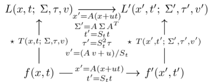
Image data are subject to natural image transformations, which to first-order of approximation can be modelled as a combination of three types of geometric image transformations:
-
•
spatial affine transformations , where is an affine transformation matrix,
-
•
Galiean transformations , where is a velocity vector, and
-
•
temporal scaling transformations , where is a temporal scaling factor.
Under a composition of these transformations of the form
| (5) | ||||
| (6) |
with two video sequences and related according to , the spatio-temporal scale-space representations and of and are related according to
| (7) |
provided that the parameters of the receptive fields are related according to
| (8) | ||||
| (9) | ||||
| (10) |
This result can be proved by composing the individual image transformations in cascade, as treated in Lindeberg [Lindeberg, 2023a].
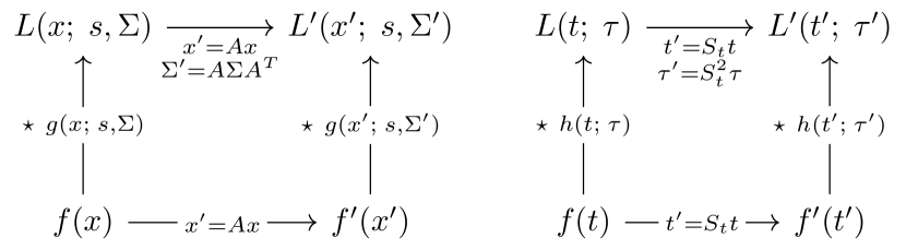
In practice, this result means that if spatio-temporal video data are subject to these classes of natural image transformations, it will always be possible to capture these transformations in the receptive field responses, provided that the parameters of the receptive fields are matched accordingly. Figure 1 illustrates the covariance property in a commutative diagram. Such a matching property can substantially improve the performance of computer vision algorithms operating on spatio-temporal receptive fields. We will next extend this result to leaky integrator neuron models and event-driven computations.
2.3 Temporal scale covariance for leaky integrator models
Gaussian kernels are symmetric around the origin and therefore impractical to use as temporal kernels in real-time situations, because they violate the principle of temporal causality. Lindeberg and Fagerström [Lindeberg and Fagerström, 1996] showed that one-sided, truncated exponential temporal scale-space kernels constitute a canonical class of temporal smoothing kernels, in that they are the only time-causal kernels that guarantee non-creation of new structure, in terms of either local extrema or zero-crossings, from finer to coarser levels of scale:
| (11) |
where the time constant represents the temporal scale parameter corresponding to in (2).
Coupling such temporal filters in parallel, for , yields a temporal multi-channel representation in the limit when :
| (12) |
A specific temporal scale-space channel representation for some signal [Lindeberg and Fagerström, 1996, Eq. (14)] can be written as
| (13) |
Turning to the domain of neuron models, a first-order integrator with a leak has the following integral representations for a given time , time constant and some time-dependent input [Gerstner et al., 2014, Eq. (1.11)]:
| (14) |
This precisely corresponds to the truncated exponential kernel in (11). Inserting into (13), we apply the temporal scaling operation for a temporal scaling factor to the temporal input signals :
| (15) | ||||
where the step (1) sets , , and . This establishes temporal scale covariance for a single temporal filter , while a set of temporal filters will be scale-covariant across multiple scales, provided the scales are logarithmically distributed [Lindeberg, 2023a, section 3.2].
2.4 Temporal scale covariance for leaky integrate-and-fire models
Continuing with the thresholded model of the first-order leaky integrator equation, we turn to the Spike Response Model [Gerstner et al., 2014]. This model generalizes to numerous neuron models, but we will restrict ourselves to the leaky integrate-and-fire equations (given in the Supplementary Material, section D), which can be viewed as the composition of three filters: a membrane filter , a threshold filter , and a membrane reset filter . The membrane filter and membrane reset filter describe the subthreshold dynamics as follows:
| (16) |
In the case of the leaky integrate-and-fire model, we know that the resetting mechanism, as determined by , depends entirely on the spikes, and we can decouple it from the spike function . If we further assume that the membrane reset follows a linear decay, governed by a time constant , of the form described in equation (29) in the Methods section, we arrive at the following formula for the leaky integrate-and-fire model:
| (17) |
Considering a temporal scaling transformation and for the temporal signals in the concrete case of , we follow the steps in equation (15):
| (18) | ||||
This shows that a single leaky integrate-and-fire filter is scale-covariant over time, and can be extended to a spectrum of temporal scales as above. Combined with the spatial affine covariance as well as Galilean covariance from equation (7), this finding establishes spatio-temporal covariance to spatial affine transformations, Galilean transformations and temporal scaling transformations in the image plane for leaky integrators and leaky integrator-and-fire neurons.
2.5 Initializing deep networks with idealized receptive fields
It is well known that spiking neural networks are comparatively harder to train than non-spiking neural networks for event-based vision, and they are not yet comparable in performance to methods used for training non-spiking deep networks [Neftci et al., 2019, Schuman et al., 2022]. To guide the training process for spiking networks, we propose to initiate the receptive fields with priors according to the idealized model for covariant spatio-temporal receptive fields. Following this idea, we used the purely spatial component of the spatio-temporal receptive fields by scale-normalized affine directional derivative kernels according to [Lindeberg, 2021, Equation (31) for ]
| (19) |
where
-
•
and denote directional derivatives in directions and parallel to the two eigendirections of the spatial covariance matrix ,
-
•
and denote the orders of spatial differentiation and
-
•
and denote spatial scale parameters in these directions, with and denoting the eigenvalues of .
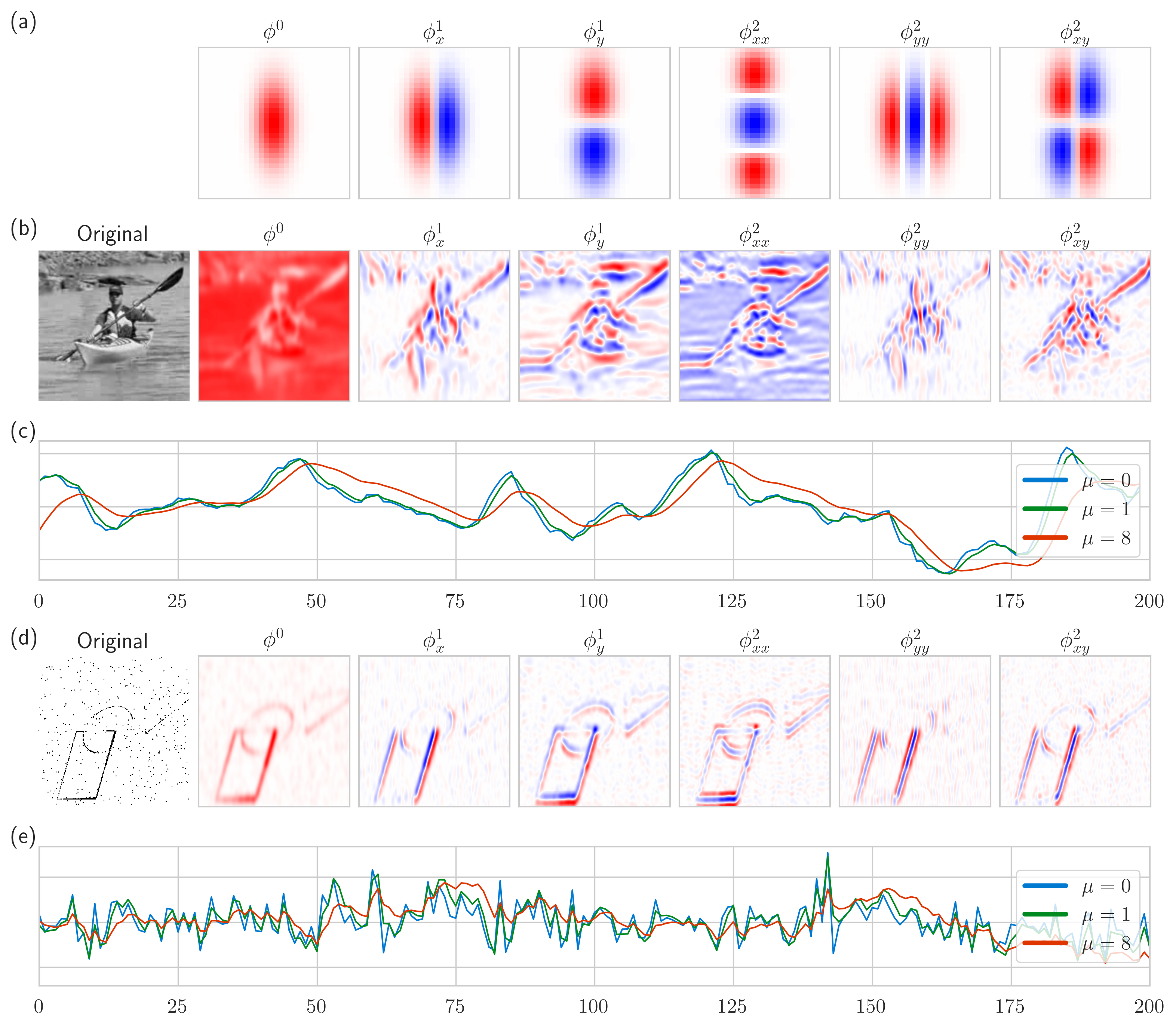
This receptive field model directly follows the spatial component in the covariant receptive field model in Section 2.2, while restricted to the special case when the image velocity parameter , and complemented with spatial differentiation, to make the receptive fields more selective. Receptive fields from this family have been demonstrated to be very similar to the receptive fields of simple cells in the primary visual cortex (see Figures 16 and 17 in [Lindeberg, 2021]). For the temporal scales, we initialize logarithmically distributed time constants in the interval for the leaky integrate-and-fire neurons, as described Section 4.1. Figure 2 (a) visualizes a subset of the spatial receptive fields that we used in the experiments. Panels (b) and (d) visualize the convolving of the spatial receptive fields with conventional image data and event data, respectively, and panels and (c) and (e) show the temporal traces change according to time scale. providing an implicit stabilization mechanism for the event-based data.
2.5.1 Experimental results
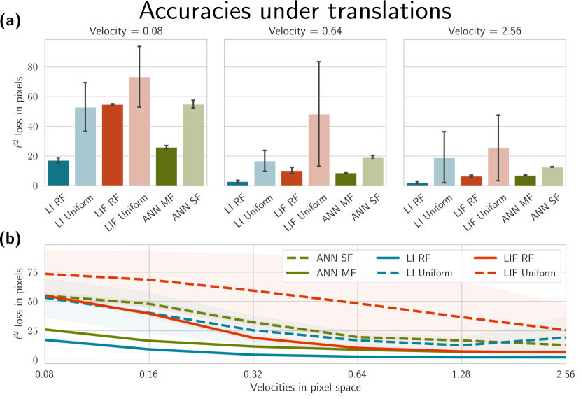
We measure the effect of the initialization scheme by constructing a simple convolutional model (see Methods Section 4.4) trained to track event-based shapes subject to affine transformations, moving according to a set of 6 logarithmically distributed velocities over time (see Figure 6). We use three subsequent temporal scaling layers, effectively allowing the model to operate on a discretized space of scales ranging over the interval , as described in Section 4.4 and shown in Figure 7. The time constants in the leaky-integrator (LI) and the leaky integrate-and-fire (LIF) models are either initialized logarithmically according to scale-space theory (see Section 4.1) or uniformly distributed.
The results in Figure 3 (a) shows that the neuromorphic models benefit significantly from the initialization scheme. Concretely, we observe that the initialization of the parameters provides a better performance, even though the model is optimized via backpropagation through time. The effect is particularly noticeable in the low-velocity setting where the signal is very sparse: the leaky integrator initialized according to theory outperforms the uniform initialization by a large margin.
Furthermore, the leaky integrator outperforms the leaky integrate-and-fire integrator, particularly in the likely because the integration scheme and optimization process is simpler. To differentiate the jumps in the thresholded leaky integrate-and-fire model, we use surrogate gradients which are, by definition, imprecise approximations [Neftci et al., 2019].
Figure 3 further compares the neuromorphic models against a non-neuromorphic baseline using rectified linear units (ReLU) instead of the temporal receptive fields (detailed in the Methods Section 4.4). A direct comparison to the single-frame ANN is strictly unfair, since ReLU models are stateless, unlike the leaky integrators. Therefore, we include an additional multi-channel model that is exposed to six frames in the past, effectively allowing the model to aggregate images in time (see Methods Section 4.4). Both the leaky-integrator and leaky integrate-and-fire models outperform the multi-frame ANN model for velocity , despite the fact that the ANN model has access to the complete and undiminished history.
For lower velocities, the leaky integrate-and-fire model falls behind; the signal becomes too sparse for the model to effectively integrate, and simple feed-forward architecture cannot cancel out the noise. Despite this, the model competes with the dense ANNs while operating with more than a 99.5% sparse signal (see Section 4.3).
2.6 Tracking performance under geometric image transformations
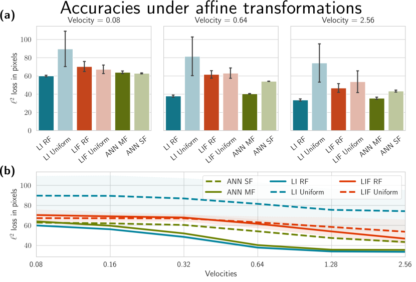
We proceed to test the covariance properties of our model for affine transformations. The affine case is more challenging than the translation setting above, but also the most realistic due to its close relation to image transformations. Figure 4 (a) shows the prediction accuracies of the models subject when trained on a dataset where shapes are subject to fully affine transformations at different velocities. Firstly, we observe higher errors than the translation case which is expected since we are applying the same model to a significantly more complex task. Secondly, we observe the same effect of the initialization scheme as in the translation case: the leaky integrator initialized according to theory outperforms the uniform initialization. The effect for the leaky integrate-and-fire model is less pronounced than in the translation case, particularly for sparser signals. Thirdly, the leaky integrator outperforms the naive ANN baseline. We ascribe this to the logarithmically distributed memory in the neuromorphic model, naïvely because it is the only difference between the models, but also because it aligns with our theoretical understanding of joint spatio-temporal covariance. Figure 2 (c) and (e) shows the importance of the temporal component for event-based vision: temporal covariance is critical to create stable representations, in particular when the input is sparse and noisy.
3 Discussion
We presented a theoretically well-founded model for covariant spatio-temporal receptive fields under geometric image transformations and temporally scaled signals, involving leaky integrator and leaky integrate-and-fire neuron models over time. We hypothesized that the initialization of spiking event-driven deep networks with priors from idealized receptive fields improves the training process. We tested our hypothesis on a coordinate regression task where simulated event-based shapes move according to translation and affine transformations. The experiments agreed with the theoretical prediction in that correctly initialized spatio-temporal fields markedly improve the training process for neuromorphic networks. They also showed that the spatio-temporal receptive fields provided a clear advantage compared to baseline ANN models, despite the ANN having access to a complete history of recent inputs. The effect for the spiking network was less pronounced for the affine transformations, which we attribute to the increased complexity of the task along with the complexity of training with surrogate descent.
We set out to study principled methods of computation in neuromorphic systems and argue our findings carry two important implications. Firstly, we have conceptually extended the scale-space framework to spiking neuromorphic primitives, which provides an exciting direction for principled computation in neuromorphic systems. Consequently, we can begin to explore the large literature around scale-space and conventional computer vision in the context of neuromorphic computing, such as covariant geometric deep learning, which have been hugely successful in computer vision [Cohen and M. Welling, 2016, Bekkers, 2020], polynomial basis expansions for memory representations, known as state space models [Voelker et al., 2019, Gu et al., 2020], and reinforcement learning [Howard et al., 2023]. Second, we uncover and exploit powerful intrinsic computational functions of neural circuits. Our networks operate on real-time data without temporal averaging and can already now translate to neuromorphic hardware via the Neuromorphic Intermediate Representation [Pedersen et al., 2023a]. This carries immediate value for event-based vision tasks and signal processing in real-time settings, where resources are scarce and necessarily time-causal. Competing with the performance of ANNs in event-based vision tasks is a crucial step towards the serious use of neuromorphic systems for real-world applications.
The experiments are designed to elicit the qualitative differences needed to experimentally test our hypotheses. The simplistic four-layer model is chosen to provide clear and interpretable results and is expected to achieve below state-of-the-art performance. Further work is needed to explore the full potential of this work, including more complex tasks, larger networks, and more sophisticated training methods.
On a broader note, the receptive fields presented here strongly resemble those in the primary visual cortex, and there is a well established link between scale-space theory and biological vision systems [Lindeberg, 2021]. The covariance properties in event-based computation we studied here align well with experimental findings around time-invariant neural processing [Gütig and Sompolinsky, 2009, Jacques et al., 2022], episodic memory “spectra” [Bright et al., 2020], and intrinsic coding of time scales in neural computation [Goel and Buonomano, 2014, Lindeberg, 2023b].
4 Methods
4.1 Spatio-temporal receptive fields
Lindeberg and Gårding [Lindeberg and Gårding, 1997] established a relationship between two scale-space representations under linear affine transformations [Lindeberg, 2013]. Concretely, if two spatial images and are related according to , and provided that the two associated covariance matrices and are coupled according to [Lindeberg and Gårding, 1997, Eq. (16)],
| (20) |
then two spatially smoothed scale-space representations, and , are related according to,
| (21) |
where parameterizes scale. When scaling from to by a spatial scaling factor of , we can relate the two scales by in the following scale-space representations [Lindeberg, 2023a, Eqs. (35) & (36)]
| (22) |
We exploit these relationships to initialize our spatial and temporal receptive fields by sampling across the parameter space for the spatial affine and temporal scaling operations.
For the spatial transformations, we sample the space of covariance matrices for Gaussian kernels parameterized by their orientation, scale, and skew up to their second derivative. For computing directional derivatives from the images smoothed by affine Gaussian kernels, we apply compact directional derivative masks to the spatially smoothed image data, according to Section 5 in [Lindeberg, 2024], which constitutes a computationally efficient way of computing multiple affine-Gaussian-smoothed directional derivatives for the same input data. Examples of spatial Gaussian derivative kernels and their directional derivatives of different orders are shown in Figure 2 (a). Combined with the convolutional operator, this guarantees covariance under natural image transformations according to Equation (21) in [Lindeberg, 2023a].
To handle temporal scaling transformations, we choose time constants according to a geometric series, which effectively models logarithmically distributed memories of the past [Lindeberg, 2023b, Eqs. (18)-(20)]
| (23) |
where is a distribution parameter that we set to , is the number of scales, and is the maximum temporal scale. Further details are available in Supplementary Material Section B.1.
This logarithmic space of scales which guarantees time-causal covariance for temporal image scaling operations [Lindeberg and Fagerström, 1996, Lindeberg, 2023a].
4.2 Spiking neuron models

We use the leaky integrate-and-fire formalization from Lapicque [Blair, 1932, Abbott, 1999], stating that a neuron voltage potential evolves over time, according to its time constant, , and some input current
| (24) |
with the Heaviside threshold function parameterized by
| (25) |
and a jump condition for the membrane potential, which resets to when the threshold is crossed
| (26) |
The firing part of the leaky integrate-and-fire model implies that neurons are coupled solely at discrete events, known as spikes.
4.2.1 Spike response model
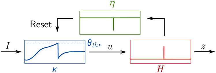
The Spike Response Model describes neuronal dynamics as a compositions of filters [Gerstner et al., 2014], a membrane filter (), a threshold filter (), and a membrane reset filter () shown in Figure 5. Consider a reset filter () applied to a spike generating function () and a subthreshold integration term () given some input current ():
| (27) |
The reset filter, , is the resetting mechanism of the neuron, that is, the function dominating the subthreshold behavior immediately after a spike. We now recast the reset mechanism as a function of time (), where denotes the time of the previous spike
| (28) |
Following [Gerstner et al., 2014, Eq. (6.33)] we define more concretely as a linearized reset mechanism for the LIF model
| (29) |
which describes the “after-spike effect”, decaying at a rate determined by . Immediately following a spike, and the kernel corresponds to the negative value of at the time of the spike, effectively resetting the membrane potential by . In the LIF model, the reset is instantaneous, which we observe when . Figure 5 shows the set of filters correspond to the subthreshold mechanism in Equation (14) (which we know to be scale covariant from Equations (15)), the Heaviside threshold, and the reset mechanism in Equation (29). We arrive at the following expression for the subthreshold voltage dynamics for the spike response model
| (30) |
where can be replaced by for the leaky integrate-and-fire model.
4.3 Dataset
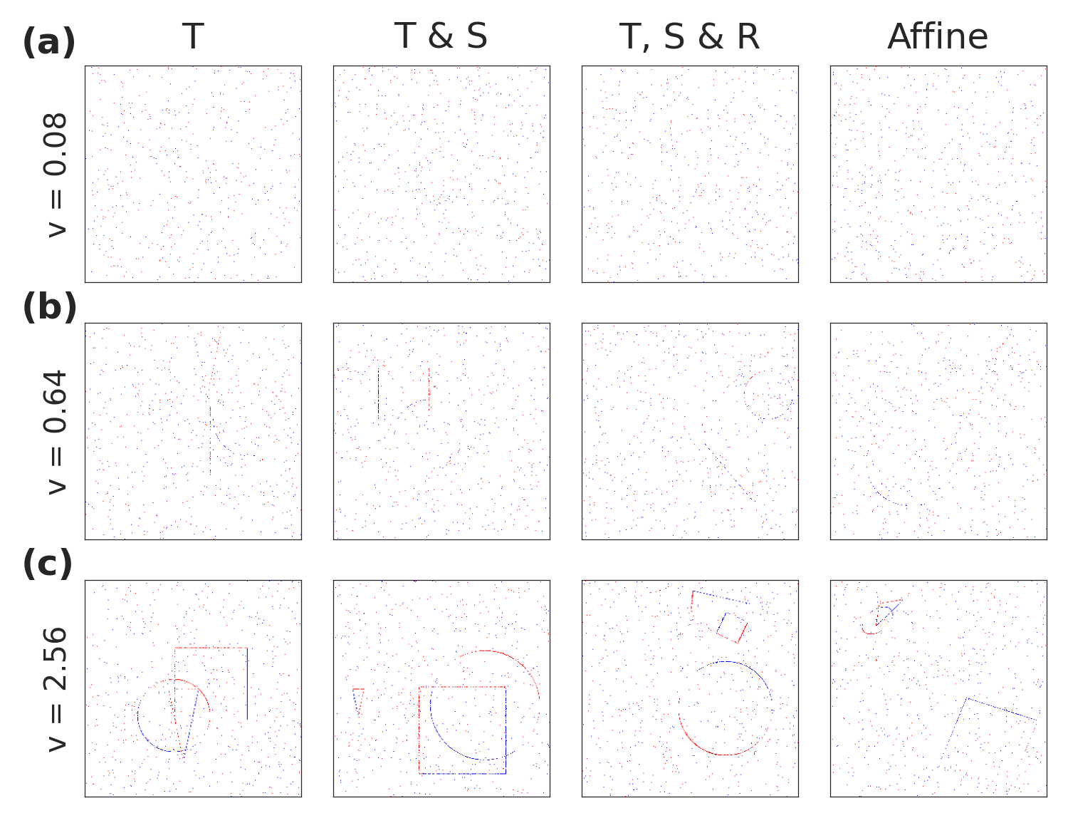
We simulate an event-based dataset consisting of sparse shape contours, as shown in Figure 6, based on Pedersen et al. [Pedersen et al., 2024]. We use three simple geometries, a triangle, a square, and a circle, that move around the scene according to four different types of transformations: translation, scaling, rotation, and affine (adding shearing). Events are generated by applying some transformation to the shapes and subtracting two subsequent frames. We then integrate those differences over time to approximate the dynamics of event cameras, until reaching a certain threshold and emitting events of either positive or negative polarity. To obtain sub-pixel accuracy we perform all transformations in a high-resolution space of pixels, which is downsampled bilinearly to the dataset resolution of .
We simulate six logarithmically distributed velocities to model varying temporal scales from 0.08 to 2.56. The velocities are normalized to the subsampled pixel space such that, for translational velocity for example, a velocity of one in the x-axis corresponds to the shape moving one pixel in the x-axis per timestep. The velocity parameterizes the sparsity of the dataset, as seen in Figure 6 panel (a), where the shape contours are barely visible compared to the faster-moving objects in panel (c). We add 5‰ Bernoulli-distributed background noise.
Note that the data is extremely sparse, even with high velocities. A temporal velocity of 0.08 provides around 3‰ activations while a scale of 2.56 provides around 4‰ activations, including noise. Furthermore, random guessing yields an average error of 152 pixels when both points are drawn uniformly from a cube [OEIS Foundation Inc., 2024, A091505]. If one of the points is fixed to the center of the cube, the error averages to 76 pixels.
4.4 Model and training
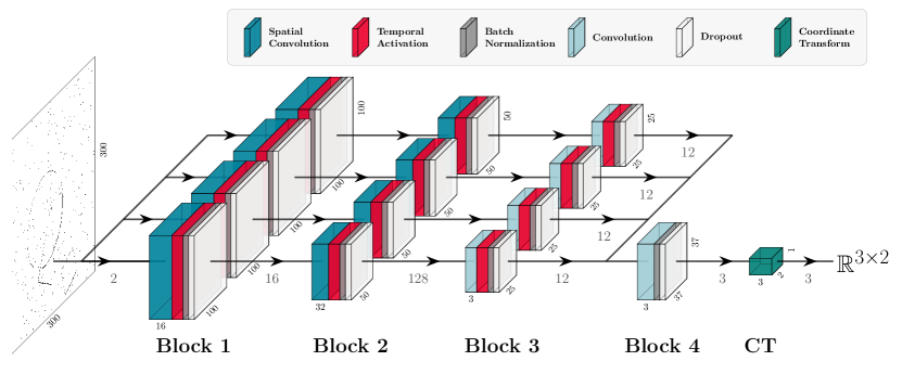
We model our network around four convolutional blocks, shown in Figure 7, with interchangeable activation functions. Each block in the model consists of a spatial convolution, an activation function, a batch normalization layer, and a dropout layer with a probability. Four different models are created. The first two such functions are the leaky integrator, coupled with a rectified linear unit (ReLU) to induce a (spatial) nonlinearity, and the leaky integrate-and-fire models. To provide baseline comparisons to stateless models, we additionally construct a stateless Single Frame (SF) model that uses ReLU activations instead of the temporal kernels and a Multiple Frame (MF) model that operates on six consecutive frames instead of one. We chose six frames in favour of the frame-based model, since an exponentially decaying leaky integrator with only retains of the signal. To convert the latent activation space from the fourth block into 2-dimensional coordinates on which we can regress, we apply a differentiable coordinate transformation layer introduced in [Pedersen et al., 2023b], that finds the spatial average in two dimensions for each of the three shapes, as shown in Figure 7. Note that the coordinate transform uses leaky integrator neurons for both the spiking and non-spiking model architectures.
The convolutions in the first two blocks are initialized according to theory as described in Section 4.1. All other parameters, both spatial and temporal, are initialized according to the uniform distribution where and is the number of input channels.
We train the models using backpropagation through time on datasets consisting of 4000 movies with 50 frames of 1ms duration, with 20% of the dataset held for model validation. The full sets of parameters, along with steps to reproduce the experiments, are available in the Supplementary Material and online at https://github.com/jegp/nrf.
5 Acknowledgements
The authors gratefully acknowledge support from the EC Horizon 2020 Framework Programme under Grant Agreements 785907 and 945539 (HBP), the Swedish Research Council under contracts 2022-02969 and 2022-06725, and the Danish National Research Foundation grant number P1.
6 Reproducibility and data availability
All material, code, and data required to reproduce the results in this paper can be found at https://github.com/jegp/nrf. All simulations, neuron models, and the spatio-temporal receptive fields rely on the Norse library [Pehle and Pedersen, 2021]. The implementation of affine directional derivatives is based on the affscsp module in the pyscsp package available from https://github.com/tonylindeberg/pyscsp and some parts of the temporal smoothing operations are based on the pytempscsp package available from https://github.com/tonylindeberg/pytempscsp.
References
- [Abbott, 1999] Abbott, L. F. (1999). Lapicque’s introduction of the integrate-and-fire model neuron (1907). Brain Research Bulletin, 50(5):303–304.
- [Aimone and Parekh, 2023] Aimone, J. B. and Parekh, O. (2023). The brain’s unique take on algorithms. Nature Communications, 14(11):4910.
- [Arnold et al., 2023] Arnold, E., Böcherer, G., Strasser, F., Müller, E., Spilger, P., Billaudelle, S., Weis, J., Schemmel, J., Calabrò, S., and Kuschnerov, M. (2023). Spiking neural network nonlinear demapping on neuromorphic hardware for IM/DD optical communication. Journal of Lightwave Technology, 41:3424–3431.
- [Barranco et al., 2015] Barranco, F., Teo, C. L., Fermüller, C., and Aloimonos, Y. (2015). Contour detection and characterization for asynchronous event sensors. In 2015 IEEE International Conference on Computer Vision (ICCV), pages 486–494.
- [Bekkers, 2020] Bekkers, E. J. (2020). B-spline CNNs on Lie groups. International Conference on Learning Representations (ICLR 2020).
- [Blair, 1932] Blair, H. A. (1932). On the intensity-time relations for stimulation by electric currents. i. Journal of General Physiology, 15(6):709–729.
- [Bright et al., 2020] Bright, I. M., Meister, M. L. R., Cruzado, N. A., Tiganj, Z., Buffalo, E. A., and Howard, M. W. (2020). A temporal record of the past with a spectrum of time constants in the monkey entorhinal cortex. Proceedings of the National Academy of Sciences, 117(33):20274–20283.
- [Cohen and M. Welling, 2016] Cohen, T. and M. Welling, M. (2016). Group equivariant convolutional networks. In International Conference on Machine Learning (ICML 2016), pages 2990–2999.
- [Delbruck and Lang, 2013] Delbruck, T. and Lang, M. (2013). Robotic goalie with 3 ms reaction time at 4 CPU load using event-based dynamic vision sensor. Frontiers in Neuroscience, 7.
- [Eliasmith and Anderson, 2004] Eliasmith, E. and Anderson, C. H. (2004). Neural engineering: Computation, representation, and dynamics in neurobiological systems. IEEE Transactions on Neural Networks, 15(2):528–529.
- [Evans et al., 2022] Evans, B. D., Malhotra, G., and Bowers, J. S. (2022). Biological convolutions improve DNN robustness to noise and generalisation. Neural Networks, 148:96–110.
- [Folowosele et al., 2011] Folowosele, F., Vogelstein, R. J., and Etienne-Cummings, R. (2011). Towards a cortical prosthesis: Implementing a spike-based hmax model of visual object recognition in silico. IEEE Journal on Emerging and Selected Topics in Circuits and Systems, 1(4):516–525.
- [Fukushima et al., 1970] Fukushima, K., Yamaguchi, Y., Yasuda, M., and Nagata, S. (1970). An electronic model of the retina. Proceedings of the IEEE, 58(12):1950–1951.
- [Gallego et al., 2022] Gallego, G., Delbrück, T., Orchard, G., Bartolozzi, C., Taba, B., Censi, A., Leutenegger, S., Davison, A. J., Conradt, J., Daniilidis, K., and Scaramuzza, D. (2022). Event-based vision: A survey. IEEE Transactions on Pattern Analysis and Machine Intelligence, 44(1):154–180.
- [Gerstner et al., 2014] Gerstner, W., Kistler, W. M., Naud, R., and Paninski, L. (2014). Neuronal Dynamics: From Single Neurons to Networks and Models of Cognition. Cambridge University Press, Cambridge.
- [Ghosh et al., 2014] Ghosh, R., Mishra, A., Orchard, G., and Thakor, N. V. (2014). Real-time object recognition and orientation estimation using an event-based camera and CNN. In 2014 IEEE Biomedical Circuits and Systems Conference (BioCAS) Proceedings, pages 544–547.
- [Goel and Buonomano, 2014] Goel, A. and Buonomano, D. V. (2014). Timing as an intrinsic property of neural networks: evidence from in vivo and in vitro experiments. Philosophical Transactions of the Royal Society B: Biological Sciences, 369(1637):20120460.
- [Gu et al., 2020] Gu, A., Dao, T., Ermon, S., Rudra, A., and Re, C. (2020). HiPPO: Recurrent memory with optimal polynomial projections. (arXiv:2008.07669). arXiv:2008.07669 [cs, stat].
- [Gütig and Sompolinsky, 2009] Gütig, R. and Sompolinsky, H. (2009). Time-warp-invariant neuronal processing. PLOS Biology, 7(7):e1000141.
- [Howard et al., 2023] Howard, M. W., Esfahani, Z. G., Le, B., and Sederberg, P. B. (2023). Foundations of a temporal RL. (arXiv:2302.10163). arXiv:2302.10163 [q-bio].
- [Howard et al., 2015] Howard, M. W., Shankar, K. H., Aue, W. R., and Criss, A. H. (2015). A distributed representation of internal time. Psychological Review, 122(1):24–53.
- [Hubel and Wiesel, 1962] Hubel, D. H. and Wiesel, T. N. (1962). Receptive fields, binocular interaction and functional architecture in the cat’s visual cortex. The Journal of Physiology, 160(1):106–154.2.
- [Jacobsen et al., 2016] Jacobsen, J.-J., van Gemert, J., Lou, Z., and Smeulders, A. W. M. (2016). Structured receptive fields in CNNs. In Proc. Computer Vision and Pattern Recognition (CVPR 2016), pages 2610–2619.
- [Jacques et al., 2022] Jacques, B. G., Tiganj, Z., Sarkar, A., Howard, M., and Sederberg, P. (2022). A deep convolutional neural network that is invariant to time rescaling. In Proceedings of the 39th International Conference on Machine Learning, page 9729–9738. PMLR.
- [Koenderink, 1984] Koenderink, J. (1984). The structure of images. Biological Cybernetics, 50(5):363–370.
- [Koenderink, 1988] Koenderink, J. (1988). Scale-time. Biological Cybernetics, 58(3):159–162.
- [Koenderink and van Doorn, 1976] Koenderink, J. and van Doorn, A. J. (1976). Geometry of binocular vision and a model for stereopsis. Biological Cybernetics, 21(1):29–35.
- [Lagorce et al., 2017] Lagorce, X., Orchard, G., Galluppi, F., Shi, B. E., and Benosman, R. B. (2017). HOTS: A hierarchy of event-based time-surfaces for pattern recognition. IEEE Transactions on Pattern Analysis and Machine Intelligence, 39(7):1346–1359.
- [Lecun et al., 1998] Lecun, Y., Bottou, L., Bengio, Y., and Haffner, P. (1998). Gradient-based learning applied to document recognition. Proceedings of the IEEE, 86(11):2278–2324.
- [Lettvin et al., 1959] Lettvin, J. Y., Maturana, H. R., McCulloch, W. S., and Pitts, W. H. (1959). What the frog’s eye tells the frog’s brain. Proceedings of the IRE, 47(11):194l–1951.
- [Lindeberg, 1994] Lindeberg, T. (1994). Scale-Space Theory in Computer Vision. Springer US, Boston, M.
- [Lindeberg, 2013] Lindeberg, T. (2013). A computational theory of visual receptive fields. Biological Cybernetics, 107(6):589–635.
- [Lindeberg, 2016] Lindeberg, T. (2016). Time-causal and time-recursive spatio-temporal receptive fields. Journal of Mathematical Imaging and Vision, 55(1):50–88.
- [Lindeberg, 2021] Lindeberg, T. (2021). Normative theory of visual receptive fields. Heliyon, 7(1):e05897.
- [Lindeberg, 2022] Lindeberg, T. (2022). Scale-covariant and scale-invariant Gaussian derivative networks. Journal of Mathematical Imaging and Vision, 64(3):223–242.
- [Lindeberg, 2023a] Lindeberg, T. (2023a). Covariance properties under natural image transformations for the generalized Gaussian derivative model for visual receptive fields. Frontiers in Computational Neuroscience, 17:1189949.
- [Lindeberg, 2023b] Lindeberg, T. (2023b). A time-causal and time-recursive scale-covariant scale-space representation of temporal signals and past time. Biological Cybernetics, 117:21–59.
- [Lindeberg, 2024] Lindeberg, T. (2024). Discrete approximations of Gaussian smoothing and Gaussian derivatives. Journal of Mathematical Imaging and Vision. preprint at arXiv:2311.11317.
- [Lindeberg and Fagerström, 1996] Lindeberg, T. and Fagerström, D. (1996). Scale-space with casual time direction, volume 1064 of Lecture Notes in Computer Science, pages 229–240. Springer Berlin Heidelberg, Berlin, H.
- [Lindeberg and Gårding, 1997] Lindeberg, T. and Gårding, J. (1997). Shape-adapted smoothing in estimation of 3-D shape cues from affine distortions of local 2-D structure. Image and Vision Computing, 15:415–434.
- [Litzenberger et al., 2006] Litzenberger, M., Posch, C., Bauer, D., Belbachir, A., Schon, P., Kohn, B., and Garn, H. (2006). Embedded vision system for real-time object tracking using an asynchronous transient vision sensor. In 2006 IEEE 12th Digital Signal Processing Workshop & 4th IEEE Signal Processing Education Workshop, pages 173–178.
- [Maass, 1997] Maass, W. (1997). Networks of spiking neurons: The third generation of neural network models. Neural Networks, 10(9):1659–1671.
- [Mead, 1989] Mead, C. (1989). Analog VLSI and neural systems. Reading, Mass. Addison-Wesley.
- [Mead, 2023] Mead, C. (2023). Neuromorphic engineering: In memory of Misha Mahowald. Neural Computation, 35(3):343–383.
- [Nagaraj et al., 2023] Nagaraj, M., Liyanagedera, C. M., and Roy, K. (2023). DOTIE - detecting objects through temporal isolation of events using a spiking architecture. In 2023 IEEE International Conference on Robotics and Automation (ICRA), pages 4858–4864.
- [Neftci et al., 2019] Neftci, E. O., Mostafa, H., and Zenke, F. (2019). Surrogate gradient learning in spiking neural networks: Bringing the power of gradient-based optimization to spiking neural networks. IEEE Signal Processing Magazine, 36(6):51–63.
- [Ni et al., 2012] Ni, Z., Bolopion, A., Agnus, J., Benosman, R., and Regnier, S. (2012). Asynchronous event-based visual shape tracking for stable haptic feedback in microrobotics. IEEE Transactions on Robotics, 28(5):1081–1089.
- [OEIS Foundation Inc., 2024] OEIS Foundation Inc. (2024). The On-Line Encyclopedia of Integer Sequences. Published electronically at http://oeis.org.
- [Orchard et al., 2015] Orchard, G., Meyer, C., Etienne-Cummings, R., Posch, C., Thakor, N., and Benosman, R. (2015). HFirst: A temporal approach to object recognition. IEEE Transactions on Pattern Analysis and Machine Intelligence, 37(10):2028–2040.
- [Pedersen et al., 2023a] Pedersen, J. E., Abreu, S., Jobst, M., Lenz, G., Fra, V., Bauer, F. C., Muir, D. R., Zhou, P., Vogginger, B., Heckel, K., Urgese, G., Shankar, S., Stewart, T. C., Eshraghian, J. K., and Sheik, S. (2023a). Neuromorphic intermediate representation: A unified instruction set for interoperable brain-inspired computing. Number arXiv:2311.14641. arXiv. arXiv:2311.14641 [cs].
- [Pedersen et al., 2023b] Pedersen, J. E., Singhal, R., and Conradt, J. (2023b). Translation and scale invariance for event-based object tracking. In Proceedings of the 2023 Annual Neuro-Inspired Computational Elements Conference, NICE ’23, pages 79–85, New York, NY, USA. Association for Computing Machinery.
- [Pedersen et al., 2024] Pedersen, J. E., Singhal, R., and Conradt, J. (2024). Event dataset generation for galilean and affine transformations.
- [Pehle and Pedersen, 2021] Pehle, C.-G. and Pedersen, J. E. (2021). Norse - a deep learning library for spiking neural networks.
- [Porcu et al., 2021] Porcu, E., Furrer, R., and Nychka, D. (2021). 30 years of space-time covariance functions. WIREs Computational Statistics, 13(2):e1512.
- [Richards et al., 2019] Richards, B. A., Lillicrap, T. P., Beaudoin, P., Bengio, Y., Bogacz, R., Christensen, A., Clopath, C., Costa, R. P., de Berker, A., Ganguli, S., Gillon, C. J., Hafner, D., Kepecs, A., Kriegeskorte, N., Latham, P., Lindsay, G. W., Miller, K. D., Naud, R., Pack, C. C., Poirazi, P., Roelfsema, P., Sacramento, J., Saxe, A., Scellier, B., Schapiro, A. C., Senn, W., Wayne, G., Yamins, D., Zenke, F., Zylberberg, J., Therien, D., and Kording, K. P. (2019). A deep learning framework for neuroscience. Nature Neuroscience, 22(11):1761–1770.
- [Schaefer et al., 2022] Schaefer, S., Gehrig, D., and Scaramuzza, D. (2022). AEGNN: Asynchronous event-based graph neural networks. IEEE Conference on Computer Vision and Pattern Recognition (CVPR).
- [Schoenberg, 1948] Schoenberg, I. J. (1948). On variation-diminishing integral operators of the convolution type. Proceedings of the National Academy of Sciences of the United States of America, 34(4):164–169.
- [Schuman et al., 2022] Schuman, C. D., Kulkarni, S. R., Parsa, M., Mitchell, J. P., Date, P., and Kay, B. (2022). Opportunities for neuromorphic computing algorithms and applications. Nature Computational Science, 2(11):10–19.
- [Sironi et al., 2018] Sironi, A., Brambilla, M., Bourdis, N., Lagorce, X., and Benosman, R. (2018). HATS: Histograms of averaged time surfaces for robust event-based object classification. In 2018 IEEE/CVF Conference on Computer Vision and Pattern Recognition, pages 1731–1740.
- [Soomro et al., 2012] Soomro, K., Zamir, A. R., and Shah, M. (2012). UCF101: A dataset of 101 human actions classes from videos in the wild. ArXiv, abs/1212.0402.
- [Tayarani-Najaran and Schmuker, 2021] Tayarani-Najaran, M. and Schmuker, M. (2021). Event-based sensing and signal processing in the visual, auditory and olfactory domain: A review. Frontiers in Neural Circuits, 15.
- [Theilman and Aimone, 2023] Theilman, B. H. and Aimone, J. B. (2023). Goemans-Williamson MAXCUT approximation algorithm on Loihi. In Proceedings of the 2023 Annual Neuro-Inspired Computational Elements Conference, NICE ’23, pages 1–5, New York, N. USA. Association for Computing Machinery.
- [Uhr, 1972] Uhr, L. (1972). Layered ’recognition cone’ networks that preprocess, classify and describe. IEEE Trans. Comput., C-21:pp. 759–768.
- [Voelker et al., 2019] Voelker, A., Kajic, I., and Eliasmith, C. (2019). Legendre memory units: Continuous-time representation in recurrent neural networks. Neurips.
- [Witkin, 1987] Witkin, A. P. (1987). Scale-Space Filtering, pages 329–332. Morgan Kaufmann, San Francisco (CA).
- [Worrall and Welling, 2019] Worrall, D. E. and Welling, M. (2019). Deep scale-spaces: Equivariance over scale. In Neural Information Processing Systems, volume 32.
- [Zhao et al., 2015] Zhao, B., Ding, R., Chen, S., Linares-Barranco, B., and Tang, H. (2015). Feedforward categorization on aer motion events using cortex-like features in a spiking neural network. IEEE Transactions on Neural Networks and Learning Systems, 26(9):1963–1978.
Appendix A Covariance properties in space and time


Definition A.1 (Covariance and invariance).
Given a set , the map is covariant if it obeys for all actions over . That is, there is a sense in which the map applied before the group action is comparable to its application after the group action. This is also known as equivariance. If acts trivially on , then and we call invariant to .
Definition A.2 (Translation).
A shift operation () translates a signal by a translation offset according to .
Definition A.3 (Scaling).
The scaling operation () scales a signal by a spatial scaling factor defined by .
Definition A.4 (Rotation).
Rotations rotate a signal around its origin by an angle . In two dimensions, when , we describe this in matrix form
| (31) |
Definition A.5 (Shearing).
The shear operation () translates a signal parallel to a given line. In two dimensions, the shear operation can be defined using the shear matrix parallel to either the horizontal
| (32) |
or vertical
| (33) |
axis.
Definition A.6 (Affine transformation).
We define an affine transformation as any map that sends a point in a vector space to another point in that same vector space. Affine transformations are the most general type of linear transformation, and include arbitrary compositions of translations, scalings, rotations, and shearings. For image transformations in two dimensions, an affine transformation in matrix form () is given by
| (34) |
Definition A.7 (Galilean transformation).
Newtonian physics tells us that two reference frames with an -dimensional spatial component () and temporal component () are related according to
| (35) | ||||
where is the relative velocity for each dimension . In the case of two spatial dimensions () and one temporal dimension, we describe the relationship between two points in space-time as follows [Lindeberg, 2023a, Eq. (20)]
| (36) |
Following the above definitions of covariance and transformations, we distinguish between invariance as well as covariance properties for affine spatial transformations, temporal scaling, and spatio-temporal Galilean transformations.
Appendix B Covariance properties in scale-space representations
Scale-space theory provides a means to represent signals at varying spatial or temporal scales. The covariance properties of the scale-space representations arrive from the commutative relationships shown in Figure 9, which we will elaborate and expand below. Given a continuous signal , we define the scale-dependent scale-space representation , parameterized by a scale , as the convolution integral with scale-dependent kernels [Lindeberg, 2023b]
| (37) |
For this property to hold, the kernel must retain or diminish variations, such that the changes in sign values for any signal sequence following the kernel application is less than or equal to the number of changes in sign value before that kernel has been applied. Specifically, if we, following Schoenberg [Schoenberg, 1948], define a “sign change detection function” , that finds the number of times a function changes sign given the sequence , and require that
| (38) |
This condition is met if and only if has a bilateral Laplace transform of the form
| (39) |
for , , , , are real, and assuming converges [Schoenberg, 1948]. Over the spatial domain, the Gaussian kernel for some signal and covariance matrix
| (40) |
along with its derivatives, is known to meet the above conditions [Lindeberg, 1994]. Concerning the temporal domain, it was shown by Lindeberg and Fagerström [Lindeberg and Fagerström, 1996] that if we require the temporal kernels to be time-causal, in the sense that they do not access values from the future in relation to any time moment, then convolutions with truncated exponential kernels [Lindeberg, 2023b, Eq. (8)]
| (41) |
by both necessity and sufficiency constitute the class of time-causal temporal scale-space kernels.
B.1 Temporal scale covariance for the causal limit kernel
The Gaussian kernel does not immediately apply to the temporal domain because it relies on future, unseen, signals, which is impossible in practice [Koenderink, 1988]. Instead, based on the above cited classification of time-causal scale-space kernels [Lindeberg and Fagerström, 1996, Lindeberg, 2016, Lindeberg, 2023b], convolutions with truncated exponential kernels
| (42) |
coupled in cascade, where are a temporal time constants, lead to the formulation of a temporal scale-space representation.
Note that we assume normalization, such that . By composing truncated exponential kernels in cascade, in the limit when trends to , Lindeberg [Lindeberg, 2016, Eq. (38)] introduces a “limit kernel” in the Fourier domain
| (43) | ||||
where the temporal scaling parameter, for scale levels, is distributed according to integer powers of the distribution parameter following for . Scaling with some factor ( denoting time), we see that [Lindeberg, 2016, Eq. (43)]
| (44) | ||||
The scale-space representation of a given signal by a scaling factor such that and is then [Lindeberg, 2016, Eq. (45)]
| (45) |
Covariance between smoothing representations and follows, again under logarithmic distribution of scales
| (46) |
where is the temporal scale and denotes a temporal rescaling factor . Returning to the temporal domain, this implies a direct relationship between neighboring temporal scales [Lindeberg, 2023a, Eq. (41)]
| (47) |
with the following scaling property
| (48) |
can be understood as a scale-covariant time-causal limit kernel, because it “obeys a closedness property over all temporal scaling transformations with temporal rescaling factors () that are integer powers of the distribution parameter ” [Lindeberg, 2023a, p. 10].
B.2 Covariance over joint spatial and temporal transformations
We now want to derive a single kernel that is provably covariant to spatial affine and Galilean transformations as well as temporal scaling transformations. With the addition of time, the spatial and temporal signals are no longer separable. Instead, we look to Newtonian physics, where relative motions between two frames of reference are described by Galilean transformations according to (35). Directly building on the (spatial) Gaussian kernel (40) and the time-causal limit kernel (47), we can, following [Lindeberg, 2016], establish spatio-temporal receptive fields as their composition
| (49) |
The corresponding scale-space representation is
| (50) |
Consider two spatio-temporal signals (video sequences) that are related according to a spatial affine transformation, a Galilean spatio-temporal transformation, and a temporal scaling transformation as follows
| (51) | ||||
| (52) |
According to Equation 21 in the main text
| (53) |
we have
| (54) | ||||
If we further set the relationships of two signals subject to Galilean and affine transformations as follows
| (55) | ||||
we can rewrite the Gaussian kernel (40) under Galilean and affine transformations as
| (56) |
For we have the corresponding spatio-temporal scale-space representation as in (50)
| (58) | ||||
and, therefore,
| (59) |
which establishes the desired covariance property for the spatio-temporal scale-space representation under affine, Galilean, and temporal scaling transformations, as shown in Figure 1 in the main text. This result also holds for the temporal Gaussian kernel (40) or truncated exponential kernel (42) by relating .
B.3 Temporal scale covariance for parallel first-order integrators
Consider a parallel set of temporal scale channels with a single time constant for each parallel timescale “channel”, modelled as a truncated exponential kernel as in equation (42):
| (60) |
for [Lindeberg, 2013, Eq. (16)] Each “channel” would assign a unique temporal scale-representation of the initial signal with a delay and duration, parameterized by . We denote a temporal scale-space channel representation for some signal
| (61) |
and observe the direct relation under a temporal scaling operation for two functions
| (62) | ||||
where step (1) sets , , and . A single filter is thus scale-covariant for the scaling operation , and a set of filters () will be scale-covariant over multiple scales, provided the logarithmic distribution of scales as in equation (46), and for scaling factors that are integer powers of the ratio between the time constants of adjacent scale levels.
Appendix C Temporal scale covariance for leaky integrators
This section establishes temporal scale covariance for leaky integrators by demonstrating that they are special cases of a first-order integrator, after which the temporal scale covariance guarantees for first-order integrators apply, as in Section B.3.
A linear leaky integrator describes the evolution of a voltage characterized by the following first-order integrator
| (63) |
where is a time constant controlling the speed of the integration, is the “resting state”, or target value of the neuron it will leak towards, is a linear resistor, and describes the driving current [Gerstner et al., 2014]. Assuming and we arrive at [Gerstner et al., 2014, Eliasmith and Anderson, 2004]
| (64) |
This is precisely the first-order integrator in the form of equation (42), and the temporal scale covariance from equation (62) follows.
Appendix D Temporal scale covariance for thresholded leaky integrators
This section establishes temporal scale covariance for thresholded linear leaky integrators. We first establish the usual, discrete formulation of thresholded leaky integrator-and-fire models and later introduce the spike response model that generalizes the neuron model as a set of connected filters. Finally, we build on the proof for the causal first-order leaky integrator above to establish temporal scale covariance for leaky integrate-and-fire models.
The leaky integrate-and-fire model is essentially a leaky integrator with an added threshold [Gerstner et al., 2014], which discretizes the activation using the Heaviside function
| (65) |
parameterized over some threshold value . When , we say that the neuron “fires”, whereupon the integrated voltage (its membrane potential) resets to :
| (66) |
The total dynamics of the leaky integrate-and-fire neuron model can be summarized as three equations capturing the subthreshold dynamic from equation (64), the thresholding from equation (65), and the reset from equation (66) [Gerstner et al., 2014].
It is worth noting that the threshold in the continuous case is a simplification of the dirac delta function defined as
| (67) |
where is a normalized Gaussian kernel. Integrating over time, we therefore have
| (68) |
Hence the “spike” () in equation (65): any layer following a thresholded activation function will be subject to a series of these unit impulses over time. As such, the neuron activation output function can be written as a sum of unit impulses over time [Gerstner et al., 2014]
| (69) |
D.1 Spike response model
This formulation generalizes to numerous neuron models, but we will restrict ourselves to the LIF equations, which can be viewed as a composition of three filters: a membrane filter (), a threshold filter (), and a membrane reset filter () shown in Figure 10. The spike response model defines neuron models as a composition of parametric functions (filters) of time [Gerstner et al., 2014]. The membrane filter and membrane reset filter describes the subthreshold dynamics as follows:
| (70) |
The reset filter, , can be understood as the resetting mechanism of the neuron, that is, the function controlling the subthreshold behaviour immediately after a spike. This contrasts the LIF formalism from equation (66) because the resetting mechanism is now a function of time instead of a constant.
Since the resetting mechanism depends entirely on the time of the threshold activations, we can recast it to a function of time (), where denotes the time of the previous spike
| (71) |
Following [Gerstner et al., 2014, Eq. (6.33)] we define more concretely as a linearized reset mechanism for the LIF model
| (72) |
The above equation illustrates how the “after-spike effect” decays at a rate determined by . Initially, the kernel corresponds to the negative value of at the time of the spike, effectively resetting the membrane potential by . In the LIF model, the reset is instantaneous, which we observe when . This is visualized in Figure 10 where the set of filters correspond to the subthreshold mechanism in equation (64) (which we know to be scale covariant from equations (62)), the Heaviside threshold in equation (65), and the reset mechanism in equation (72).
We arrive at the following expression for the subthreshold voltage dynamics of the LIF model:
| (73) |
D.2 Temporal covariance for the LIF model
We are now ready to state the scale-space representation of a LIF model as a special case of the above equation (73) where :
| (74) |
Considering a temporal scaling operations and for the functions , we follow the steps in equation (62):
| (75) | ||||
where step (1) sets , , , and . This concludes the proof that the LIF model, described as a set of linear filters, retains temporal scale covariance.