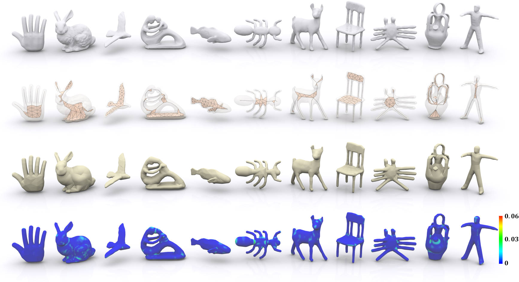
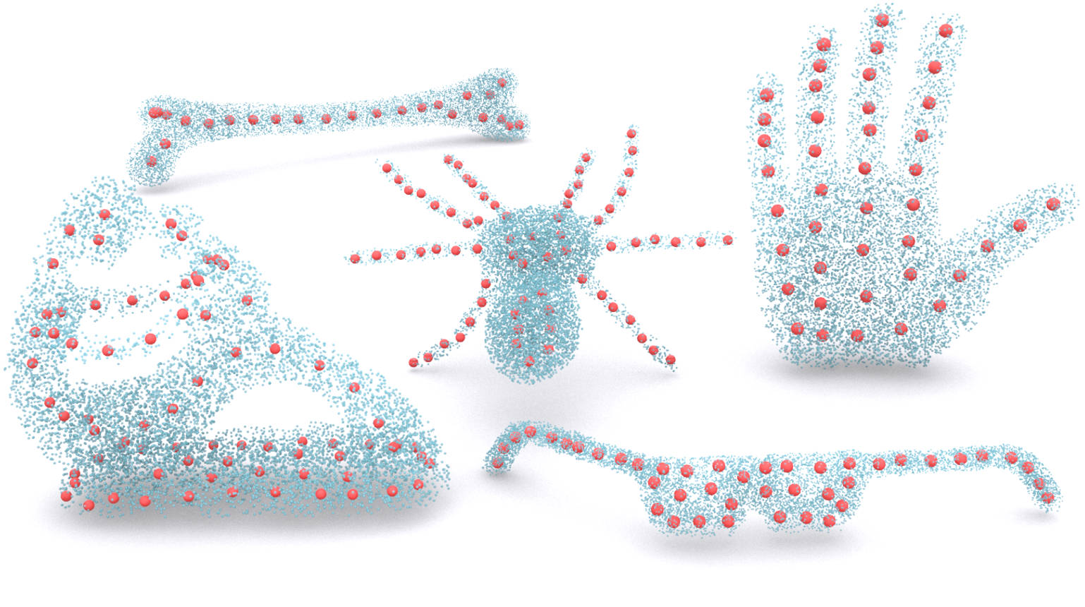
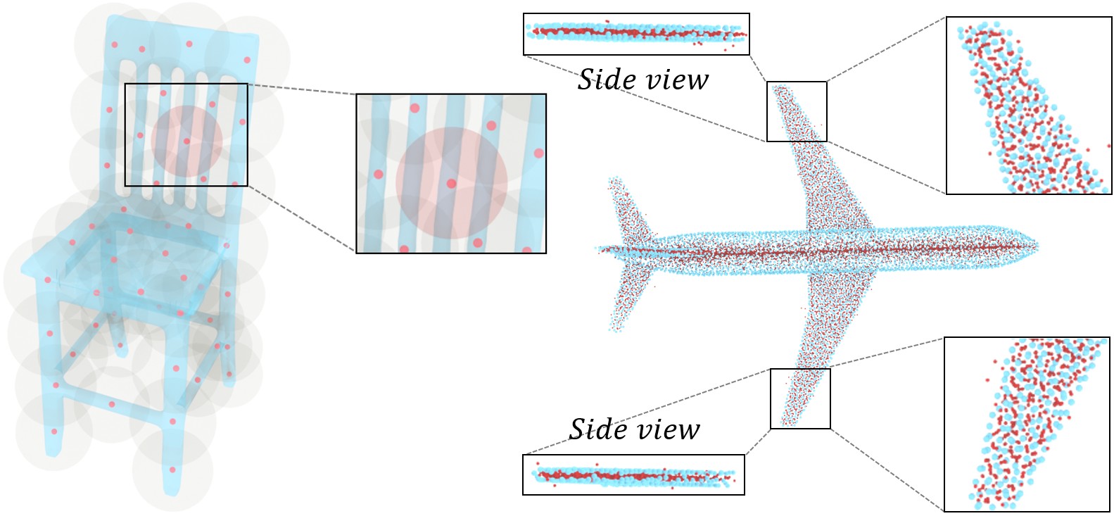
![[Uncaptioned image]](https://cdn.awesomepapers.org/papers/49feae21-a757-4b7a-a5b1-e56762f1f6f4/fig_teaser_zipped.jpg)
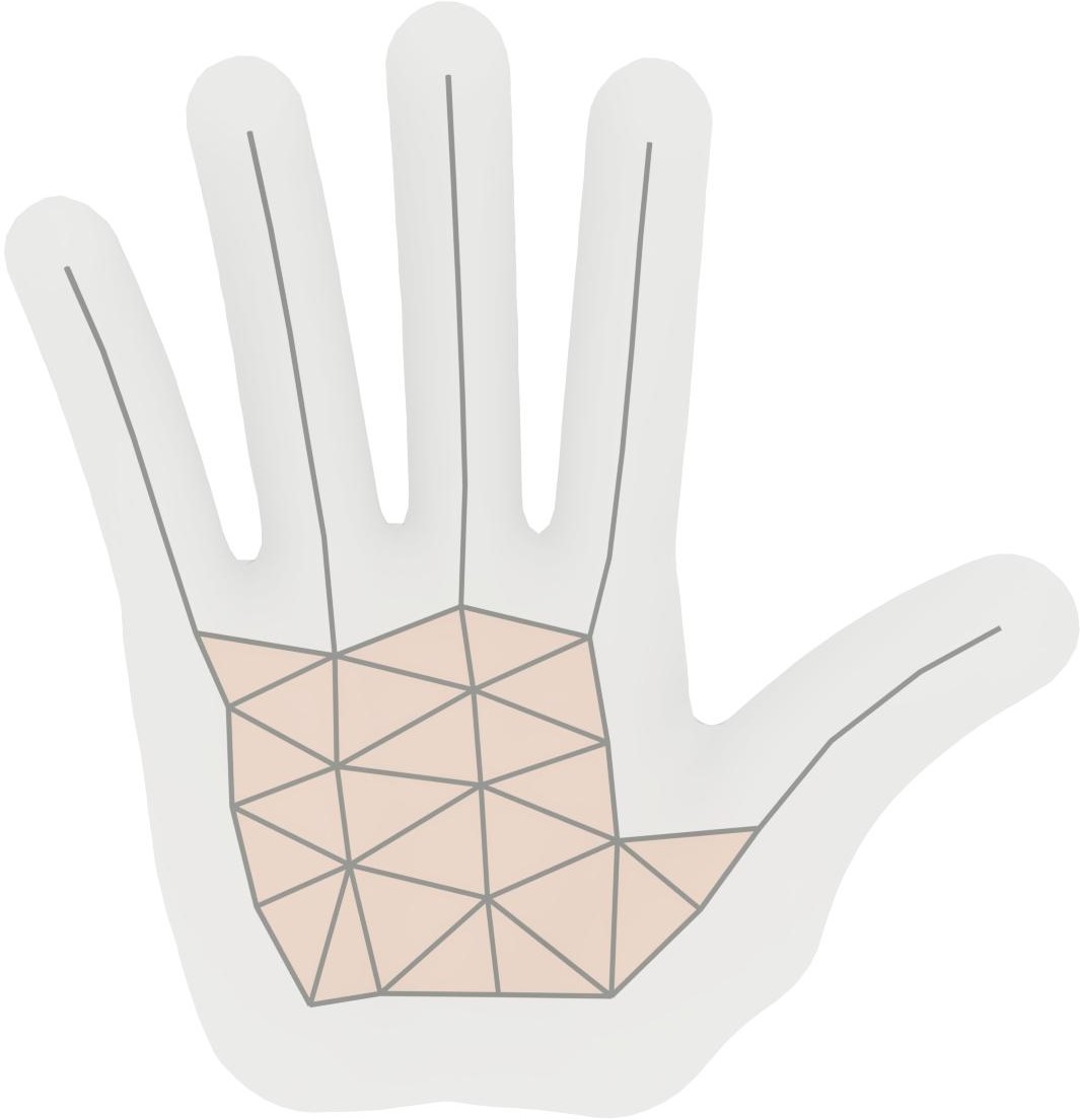
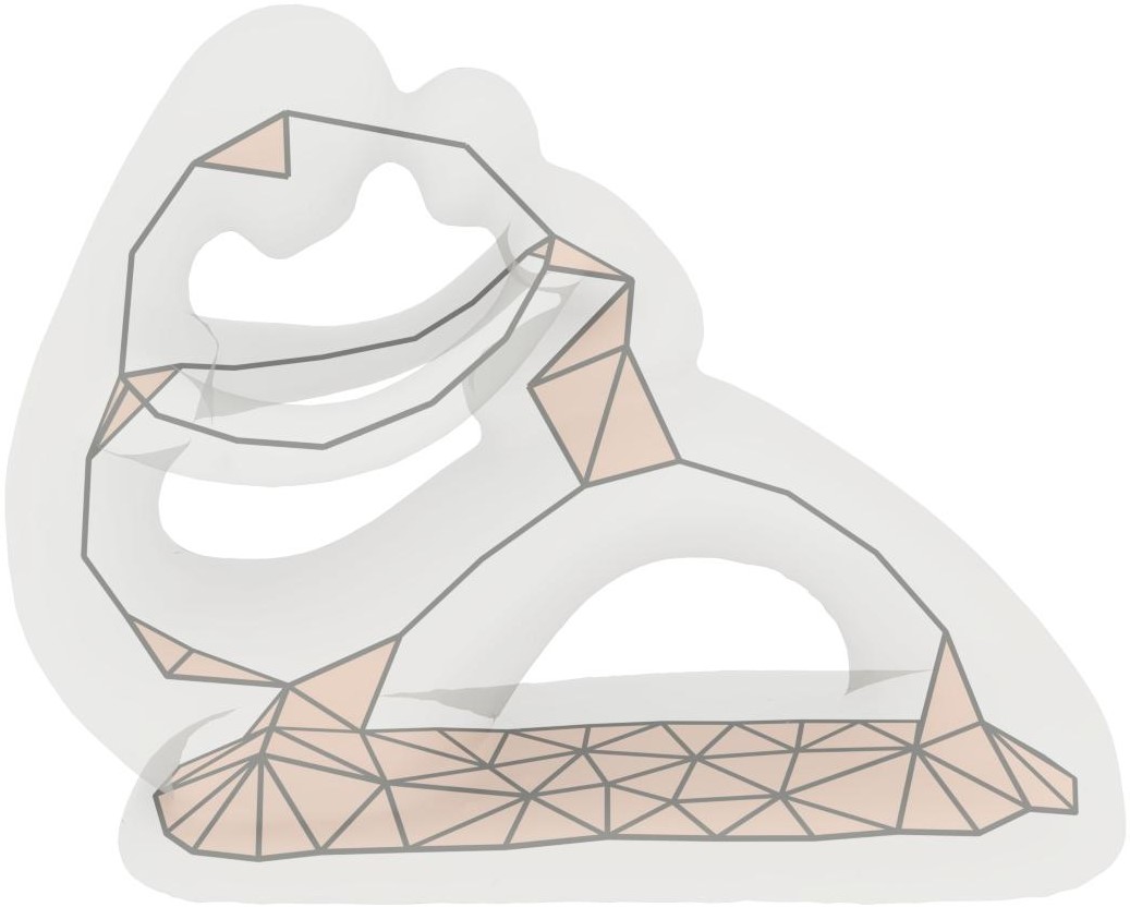
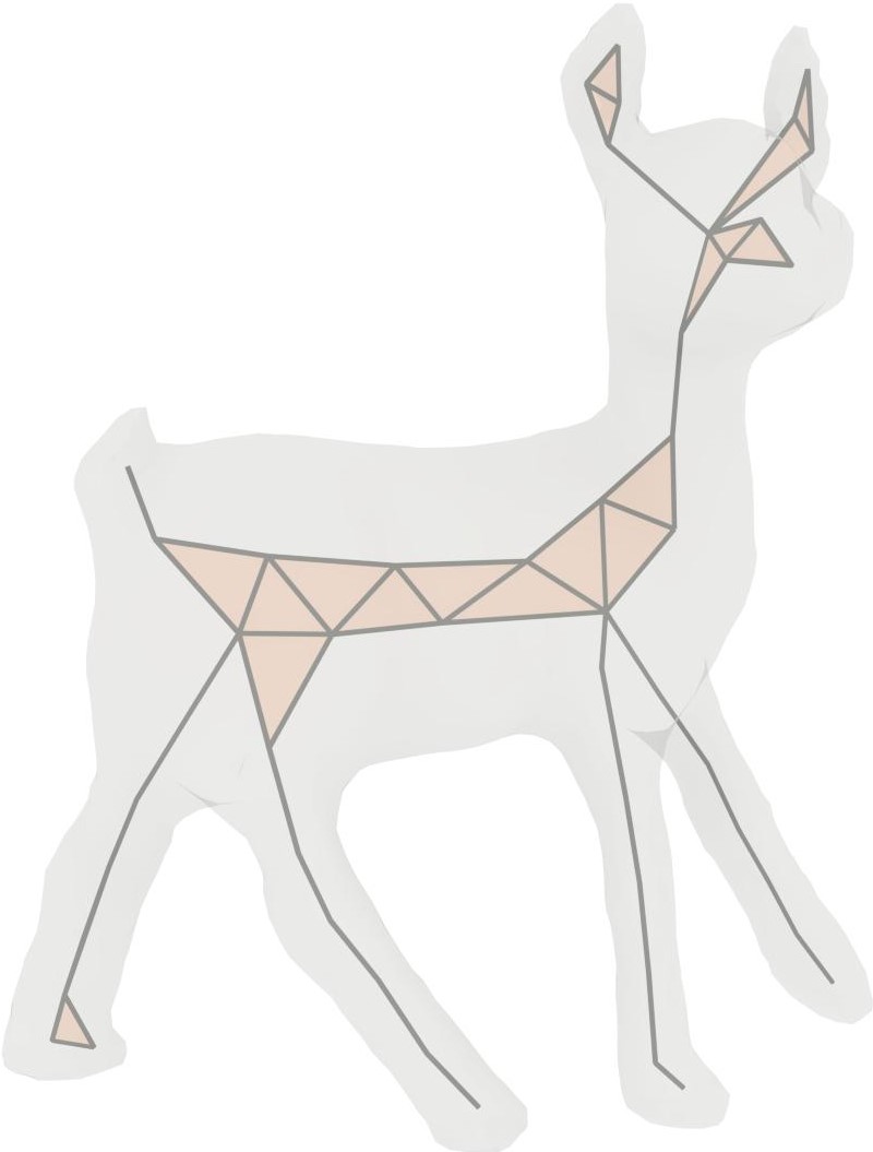
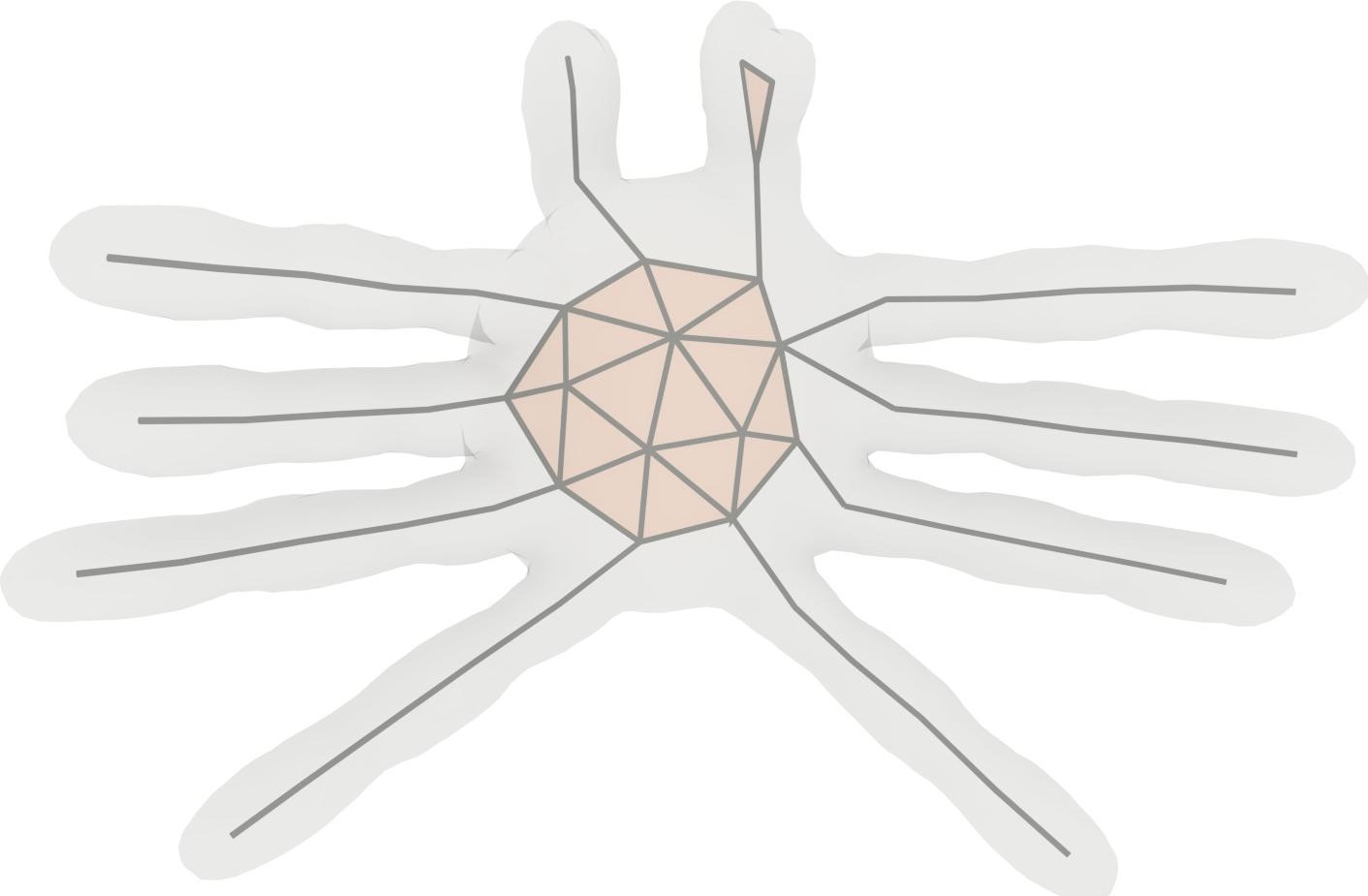
A gallery of 3D shape skeletonization results by Coverage Axis from surface mesh input.
Coverage Axis: Inner Point Selection for 3D Shape Skeletonization
Abstract
In this paper, we present a simple yet effective formulation called Coverage Axis for 3D shape skeletonization. Inspired by the set cover problem, our key idea is to cover all the surface points using as few inside medial balls as possible. This formulation inherently induces a compact and expressive approximation of the Medial Axis Transform (MAT) of a given shape. Different from previous methods that rely on local approximation error, our method allows a global consideration of the overall shape structure, leading to an efficient high-level abstraction and superior robustness to noise. Another appealing aspect of our method is its capability to handle more generalized input such as point clouds and poor-quality meshes. Extensive comparisons and evaluations demonstrate the remarkable effectiveness of our method for generating compact and expressive skeletal representation to approximate the MAT.
{CCSXML}<ccs2012> <concept> <concept_id>10010147.10010371.10010396.10010402</concept_id> <concept_desc>Computing methodologies Shape analysis</concept_desc> <concept_significance>500</concept_significance> </concept> </ccs2012> \ccsdesc[500]Computing methodologies Shape analysis
\printccsdesc1 Introduction
With the capability of effectively capturing the underlying structures of 3D shapes, skeletal representations have been an important tool in various applications of shape analysis and geometric processing, such as 3D reconstruction [WHG*15, THP*19, ACK01], volume approximation [SKS11, SCYW13], shape segmentation [LLL*20], shape abstraction [DXX*20], pose estimation [SFC*11, YRL*21] and animation [BP07, YYG18], etc.
Curve skeletons, consisting of only 1D curves, have been extensively researched [ATC*08, MWO03, TAOZ12, XZKS19] due to their simplicity and intuitiveness. Curve skeletons are usually empirically understood, while Dey and Sun [DS06] give a mathematical definition based on Medial Geodesic Function. Generally, the curve representation only applies to tubular components instead of arbitrary shapes, which thus cannot be considered as a generalized tool for shape analysis.
Another prominent example of skeletal representations is called the Medial Axis Transform (MAT) [Blu*67]. The MAT is defined by a union of the maximally inscribed balls inside the shape with the associated radius functions. Different from the curve skeleton, the MAT has a consistent definition for arbitrary shapes. In addition to curves, the MAT consists of both curve-like and surface-like structures thus leading to significantly better representational ability. That being said, the MAT is difficult to use which mainly manifests in two aspects. First, the MAT is notoriously sensitive to boundary noise, i.e., small perturbations on the boundary surface will result in dramatic changes on the medial axis. Second, the computation of the MAT usually relies on stringent requirements of the input geometry, such as the watertightness and manifoldness of the surface.
In this paper, we propose Coverage Axis, a novel and simple formulation to generate skeletal representations for 3D shapes. Our goal is to give a compact approximation of the MAT, while this approximation should inherit good geometric and topological properties of the MAT but overcome its aforementioned drawbacks.
We observe a medial sphere can be considered as an abstraction of local geometry, while the union of all the local geometries forms the entire shape. With this insight, our key idea is to formulate a Set Cover Problem, of which goal is to identify the smallest sub-collection of whose union equals the universe. Specifically, we aim to find the minimum number of dilated inner balls that cover sub-regions on the surface (i.e., sub-collection) to approximate the whole shape (i.e., universe).
This formulation inherently induces a compact and expressive representation that approximates the MAT. First, the coverage constraint enforces consistency with the shape structure. Second, selecting the fewest possible candidates for shape approximation not only gives a simplified representation, but also favors the interior points that dominate larger area, which corresponds to the definition of MAT, i.e., maximally inscribed spheres.
Compared to the existing methods that mainly focus on MAT simplification [ACK01, LWS*15, GMPW09, FLM03, DZ02, SFM07, MGP10], our method has several appealing aspects. First, its formulation is simple yet effective, which does not require any complex geometric processing nor a computationally-costly pipeline to derive skeletal points. Compared to metrics like QEM [GH97] and Spherical QEM [TGB13] which are used to construct the medial axes by only considering the local geometry, our set coverage formulation jointly leverages all the surface points and inner points for computing MAT approximation, which results in considering the global shape structure, and thus leads to a better abstraction of the overall shape as well as a shape-aware point distribution. More importantly, we can handle the input of poor-quality meshes or point clouds since our method is based on the coverage of point sets, while other algorithms usually rely on watertight surfaces with decent quality. Finally, our method takes as input a set of overfilled inner point candidates and selects the most expressive ones as the skeletal points; thus it does not necessarily need to compute a rigorously defined MAT, but can work with randomly generated points inside the input.
We demonstrate the effectiveness and robustness of our method on a variety of 3D shapes. The extensive evaluation results reveal that our novel and simple formulation for inner point selection effectively captures the global structure and the fundamental geometry of input shapes, thus providing informative skeletal representations to approximate the structure of the MAT.
2 Related Work
Curve skeletonization
Curve skeletonization has been extensively researched in computer vision and computer graphics. Traditional methods rely on hand-crafted rules to utilize geometric information for curved skeleton computation [AM96, MWO03, SLSK07, ATC*08, NBPF11, TAOZ12, XZKS19, CZC*20]. Specifically, Ma et al. [MWO03] applies using radial basis functions (RBFs) for skeleton extraction. Sharf et al. [SLSK07] adopt a deformable model evolution that captures the object’s volumetric shape and then generates the approximation for the curve skeleton. Au et al. [ATC*08] compute the skeleton via mesh extraction. Livesu et al. [LGS12] reconstruct the curve skeletons of 3D shapes using the visual hull.Mean Curvature Skeleton [TAOZ12] formulates the skeletonization problem via mean curvature flow, which drives the curvature flow towards the extreme so as to collapse the input mesh. The mesh collapse also induces an intermediate result called meso-skeleton that consists of both surface-like and curve-like structures. Recently, Cheng et al. [CZC*20] propose a method for skeletonization using the dual of shape segmentation.
At the same time, learning-based methods [XZKS19] have been proposed for predicting curve skeletons. Although curve skeletons are able to represent tubular shapes, it has issues representing arbitrary shapes, e.g., shapes with flat components.
Medial axis transform
As a more general skeletal representation, medial axis transform (MAT) [Blu*67] is able to encode arbitrary shapes with curve-like and mesh-like structures. The maximal balls defined in the volume together with their locii complete the representation of the shape.
The most commonly used technique for extracting MAT is to initialize the medial surface using the Voronoi diagrams. Then a simplified medial surface is achieved by applying optimization on spikes pruning or mesh tessellations based on various rules. Following this way, there are many existing approaches. Angle-based filtering methods [ACK01, FLM03, DZ02, SFM07] reach a simplification based on the angle formed by the point of MA and its two closest points on the boundary. These methods usually produce a simplified result with local features well preserved; however, they suffer from preserving the original topology of the objects. -medial axis methods [CL05, CCT11] are another series of methods to simplify the computation of MAT, which adopt cumradius of the closest points of a medial point as a pruning criterion. The main drawback of these methods is poor feature preserving ability at different scales [ABE09].
Compared with the aforementioned methods, Scale Axis Transform (SAT) [MGP10] prunes spikes more effectively. Unstable medial axis points are identified if the corresponding medial balls are covered by the neighboring medial balls during the multiplicative growing. However, SAT typically has a significant computational cost and tends to destroy the topology by introducing new topological structures at large scales. To overcome these issues, progressive medial axis filtration (PMAF) [FTB13] proposes to perform successive edge collapse based on sphere absorption to preserve the topology as well as improve time efficiency. Our idea also uses a dilated medial balls; we pay special attention to the relationship between inner balls and surface samples. Different from SAT that favors a dense representation with a large number of vertices on the medial axis, our method is able to yield a compact skeletal representation without destroying the shape structure.
Meanwhile, other strategies have been proposed to achieve simplified MAT, e.g., Delta Medial Axis (DMA) [MLM16], Bending Potential Ratio (BPR) pruning [SBH*11], Erosion Thickness (ET) measure [YSC*16], voxelization based -pruning [YLJ18]. The simplified MAT, without doubt, cannot reconstruct the original shape exactly, and thus Sun et al. [SCYW13] propose to control the approximation error by computing the Hausdorff distance. Rebain et al. [RLS*21] introduce medial fields derived from the MAT to represent the original shape using learning techniques.
To achieve high accurate approximation of the original shape, Li et al. [LWS*15] propose Q-MAT that adopts quadratic error metric (QEM) [GH97] for MAT simplification. As an edge collapse method, Q-MAT is fast and produces a piecewise linear approximation of the MAT. Q-MAT collapses edges based solely on local information, which sometimes leads to unreasonable spatial distribution of vertices. Also, Q-MAT is limited to 2-manifold surface scope. Additionally, Q-MAT heavily relies on a good MAT initialization; when the initial MA is low quality, Q-MAT can not produce correct results by edge collapse. Instead, we tackle this problem from a global view, which can preserve representative inner points with relatively even spatial distribution. As our method is based on the coverage of point sets, we can handle inputs of poor-quality meshes or point clouds. Furthermore, our method, as we will demonstrate, has good adaptability to low-quality candidate points. We refer readers to [TDS*16] for a detailed survey covering various forms of skeletons.
Point cloud skeletonization
Nowadays, skeletonization of point cloud is drawing people’s attention due to the easy availability of point cloud data [And09, CTO*10, LGS12, HWC*13, RAV*19, WHG*15, YYW*20]. In particular, L1-medial skeleton [HWC*13] contracts point clouds based on locally optimal projections (LOP) [LCLT07]. LSMAT [RAV*19] takes a densely sampled oriented point set as input and computes an MAT approximation on the basis of Signed Distance Function (SDF). Wu et al. [WHG*15] associates the surface points to the inner point residing on the meso-skeleton [TAOZ12]. However, represented by unstructured points, their skeletonization lacks topological constraints. Additionally, the reconstruction results of [WHG*15] are still with large error.
With the success of deep neural networks, learning-based methods have been proposed for predicting skeletons of point clouds [YYW*20, LLL*21]. P2MAT-NET [YYW*20] transforms sparse point cloud to an output set of spheres to approximate the medial balls. Point2Skeleton (P2S) [LLL*21] learns skeletal representations from generalized point clouds in an unsupervised manner. Learning-based methods do not guarantee accurate computation of geometric features. Furthermore, they often suffer from generalization ability due to the dependency on the training data.
3 Preliminaries
3.1 Medial Surface
![[Uncaptioned image]](https://cdn.awesomepapers.org/papers/49feae21-a757-4b7a-a5b1-e56762f1f6f4/fig_MAT_warpfig.jpg)
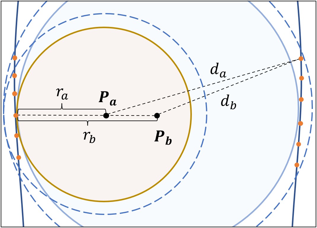
Given a closed, oriented and bounded two-manifold surface in , medial axis is defined as the locus of the center of maximally inscribed spheres that are tangent to at two or more points. The medial axis of , together with its radius function , forms the medial axis transform (MAT), denoted by a pair .
3.2 Voronoi Diagram & Power Diagram
Voronoi diagram is a partition of the domain into regions, close to a set of points called generators . Each region, also called cell, is defined as
A well-known MAT initialization technique is to use the Voronoi diagram inside a model generated by sampled points on the surface.
Power diagrams [Aur87] can be viewed as an extension of Voronoi diagrams, where each generator is equipped with a weight to control its influence. By defining the power distance between and the weighted generator to be , the cell associated with is defined by
A generator with a larger weight is more dominant, and when all the weights are equal, the Power diagram is reduced to a Voronoi diagram. In [ACK01], the approximate MAT structure is built based on regular triangulation, the dual of Power diagram, with the weights as squared radius of inside and outside poles (a subset of Voronoi vertices). Examples of a Voronoi diagram and a Power diagram are shown in Figure 1 respectively.
4 Method
Our goal is to generate a compact skeletal representation of a given 3D shape that approximates its MAT, for capturing the fundamental structure of the shape.
Our method consists of three main steps. We first generate a set of inner points as the candidate skeletal points. Then, we introduce a novel formulation called coverage axis, which is based on the set cover problem, to find a minimal sub-collection of candidates to recover the input shape. Finally, we analyze the connectivity of the selected points to form a connected structure with edges and triangles.
4.1 Inner Points Generation
Our method starts with the generation of candidate points located inside a given 3D shape. The input to our system can be either surface meshes or point clouds with normals.
For a mesh input, following a common initialization technique, we compute the Voronoi diagram of a set of points sampled on the mesh and extract the inner points, which become the candidate points of the skeleton. The inside Voronoi diagram becomes the initial coverage axis structure.
For a point cloud input (with normals), similar to a mesh input, we first compute the Voronoi diagram w.r.t. surface samples. Then, we extract the inner points as follows. We first compute its Delaunay triangulation which is the dual of the Voronoi diagram w.r.t. the input point cloud. Consider a Voronoi vertex and the vertices of its dual tetrahedron and . The candidate is considered as an inner point only if we have , . Here is the input normal of and is dot product. See more details in Appendix A. Note other inside-outside query methods such as [BDS*18] are also applicable.
The Voronoi-based point generation is based on principled geometric transform which can generate candidates with good quality. Nevertheless, note our method does not rely on strictly defined MAT for initialization. We can also randomly sample a set of points inside the shape and use them as skeleton candidates (see Sec. 6.1 for a detailed discussion). This property significantly enhances the flexibility of our method for handling various inputs in different applications.
4.2 Point Selection Based on Set Coverage
Given a set of elements (called universe) and its subsets whose union equals the universe, the set cover problem (SCP) is to identify the minimum sub-collection of these subsets whose union equals the universe. Inspired by this formulation, we now introduce our Coverage Axis. In the last step, we obtain a set of inner point candidates . We estimate the radii of these points as their closest distances to the boundary surface, resulting in candidate balls. Now we slightly dilate all the balls by adding a small value to their radii, i.e., , leading to a set of dilated balls . The dilation makes our algorithm robust to insignificant details and noise, for which we give detailed discussions later in Sec. 6.2.
Our goal is to find the minimum number of dilated balls that cover all the sampled points on the surface. For this purpose, we introduce a coverage matrix , where and are total numbers of sampled surface points and candidate skeletal points, respectively. Each element of indicates if a surface point is covered by the dilated ball :
| (1) |
Let be a decision vector, where the -th element indicates if a candidate skeletal point is selected. Now we can derive the formulation of our 0-1 integral optimization problem:
| (2) |
where is a vector of ones and is applied element-wise to the vector entries. Here we minimize the norm of the decision vector under a certain constraint. The constraint enforces each sampled point to be covered by the selected skeletal balls, which ensures consistency between the selected skeleton and the input shape. With this simple formulation, our method allows a global consideration of the overall shape structure and effectively selects the most predominant inner candidates, giving an expressive and compact skeletal representation to faithfully capture the fundamental geometry and topology. We solve Eq. 2 using Mixed-integer linear programming (MILP) solver in Matlab (MathWorks 2021). The pipeline of inner point selection is demonstrated in Figure 2. We further discuss a series of properties of our method, e.g., centrality, robustness to noise, etc., in Sec. 6.
It is notable that the constraint in Eq. 2 does not always lead to a solution. For example, if there are points not covered by any dilated balls (assume the dilation is tiny), no solution can be found. Nevertheless, this barely happens and the fixed parameters always lead to a solution for the extensive experiments as we will show later. This is owing to the proper initialization for generating inside candidates: Voronoi Diagram or densely sampled points. Voronoi Diagram produces balls maximally inscribed to the surface, thus already giving tight-fitting candidates. The randomly generated inner points are considerably dense, of which a subset approximates the vertices of the Voronoi Diagram, and the excessive balls provide abundant candidates for solving SCP.
4.3 Connection Establishment
Once the skeletal points are determined, in this step, we analyze their connectivity to form a structured mesh. Generally, if the input is a surface mesh, the topological connections of the skeletal points are easier to be derived from the surface. However, this is difficult when the input is a point cloud that only consists of unorganized points.
Considering our method flexibly allows different input types (i.e., surface mesh and point cloud) with different candidate generation strategies (i.e., Voronoi-based and random sampling), we propose to use different ways to build the connections of skeletal points. More details can be found in Appendix B.
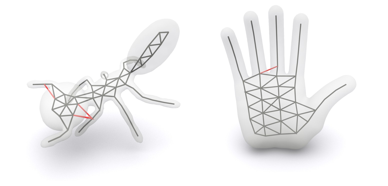
![[Uncaptioned image]](https://cdn.awesomepapers.org/papers/49feae21-a757-4b7a-a5b1-e56762f1f6f4/fig_connection.jpg)
Mesh with candidates from Voronoi diagram
This configuration usually gives the best skeletonization quality since not only the boundary surface is structured, but the inner points are derived from principled geometric transform, thus also having a good structure. Accordingly, we can obtain selected points embedded on the Voronoi diagram (the part locating inside the model). Note that such a Voronoi diagram provides a correct topological connection w.r.t. the input 3D model. We then can simplify this structure using off-the-shelf method with selected points. In this paper, we follow the edge collapse strategy of Q-MAT [LWS*15]. But the key difference is that the result selected by set coverage serves as a series of anchors; these points, like nails, are guiding the direction of further simplification so as to ensure a more reasonable distribution w.r.t. original geometry. In particular, for an edge to be collapsed, if one endpoint is not the selected point but another is, we merge the point to the selected point; if two endpoints are both selected points, we preserve this edge and skip to the next edge; if both two endpoints are not selected, we merge them to the optimal contraction target same as [LWS*15]. Meanwhile, topology preservation [DEGN98] and mesh inversion avoidance algorithm [GH97] are applied during the collapse.
More generalized configurations
This case takes the input of either mesh or point cloud, while the candidate skeletal points can be generated by Voronoi diagrams or random sampling. Different from the first case, where both inner and outside structures are well defined, it is challenging to derive precise topological connections of the skeletal points. We seek for an approximation of the MAT connection similar to [ACK01] as follows.
Suppose is the set of all selected points by set coverage. Let denotes the set of the surface. We then compute the Power diagram PD on the set of and establish the connection by extracting edges among the selected inner points on the dual of PD, regular triangulation RT. In order to suppress over-connection, we up-sample on the input point cloud following [HWG*13], leading to surface samples. These points are treated as surface points in RT during connection establishment. Note that can be adjusted accordingly during the computation of RT to achieve flexible control over the connection.
5 Experimental Results
In this section, we conduct qualitative and quantitative evaluations of the proposed method to comprehensively demonstrate its effectiveness. We implement and experiment on a computer with a 4.00 GHz Intel(R) Core(TM) i7-6700K CPU and 16 GB memory. The size of all the models are normalized to the range.
All the experimental results are generated using a consistent parameter setting, i.e., for all kinds of input, we always set . For a mesh input, we sample points from the surfaces. The resulting set is denoted by and is used to compute the Voronoi diagram, whose vertices inside the input mesh serve as candidate inner points set, denoted by . Then we sample surface points as the set to be covered in the SCP. Here is set to be less than to reduce the computational cost (see Sec. 6.5 for a detailed evaluation). The input point clouds all have points, and thus we have . Detailed analyses on these parameters and are given in Sec. 6.4.
As for evaluation metrics, besides one-sided Hausdorff distance (HD) from the input surface to the surface reconstructed by the skeleton that is employed by Q-MAT [LWS*15], we adopt two-sided Hausdorff distance since the former is not informative to fully reveal the consistency between two surfaces. We use to denote the HD from surface to reconstruction, to denote the HD from reconstruction to surface, and to represent two-sided HD.
We show a set of qualitative results on various 3D shapes in Figure Coverage Axis: Inner Point Selection for 3D Shape Skeletonization. The shape approximation results are shown in Figure 3. The reconstruction results are obtained by interpolating the medial balls based on the skeleton connectivity similar to [LWS*15]. Please refer to the Appendix for more implementation details.
5.1 Coverage Axis from Mesh Input
We conduct comparisons with representative MAT simplification methods including Q-MAT [LWS*15] and SAT [MGP10]. The errors are scaled by the length of the diagonal of the input model bounding box.
Comparison with Q-MAT [LWS*15]
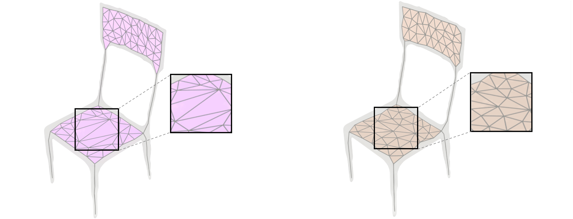
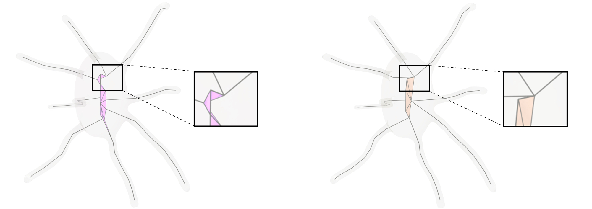
For a fair comparison, the number of vertices in the medial axis are set the same for both methods. The quantitative results are reported in Table 1. It can be seen that our method is comparable with or better than Q-MAT in terms of reconstruction error. Additionally, we conduct comparisons with Q-MAT on the robustness against the input noise, whose results are given in Sec. 6.2.
From the experiments, it is revealed that the problem with Q-MAT is that it may yield an uneven distribution of inner points in parts where the geometry is similar (Figure 4 (a) first and second row). This is because the edge collapse strategy of Q-MAT is solely based on local approximation errors, which lacks the global constraints of the whole geometry. This problem is even worse once a highly simplified representation is needed.
| Model | Q-MAT | Coverage Axis | |||||
| Ant-1 | 2.236% | ||||||
| Armodillo | 2.947% | ||||||
| Bird | 1.539% | ||||||
| Bunny | 2.526% | ||||||
| Chair-1 | 1.534% | ||||||
| Crab | 1.759% | ||||||
| Cup | 2.481% | ||||||
| Desk | 1.930% | ||||||
| Dog | 2.077% | ||||||
| Fertility | 2.703% | ||||||
| Fish | 2.325% | ||||||
| Hand-1 | 1.750% | ||||||
| Hand-2 | 1.716% | ||||||
| Human-1 | 2.729% | ||||||
| Human-2 | 1.526% | ||||||
| Human-3 | 1.788% | ||||||
| Kitten | 2.490% | ||||||
| Octopus-1 | 1.836% | ||||||
| Octopus-2 | 2.316% | ||||||
| Pig | 2.183% | ||||||
| Plane | 1.184% | ||||||
| Snake | 1.623% | ||||||
| Spectacle | 2.133% | ||||||
| Bear | 2.619% | ||||||
| Vase | 2.906% | ||||||
| Average | - | 2.264% | |||||
-
1
The number of skeletal points.
-
2
One-sided HD from surface to reconstruction.
-
3
One-sided HD from reconstruction to surface.
-
4
Two-sided HD between original surface and reconstruction.
(a) Q-MAT
(b) Coverage Axis
In contrast, our method effectively leverages the global geometric and topological features of the input shape for skeleton generation. The point selection step jointly considers the overall input points and candidates, while the selected expressive points are used as fixed anchors to preserve the global topology. Hence, the skeletal representations generated by our method are equipped with shape-aware point distributions as well as connectivity.
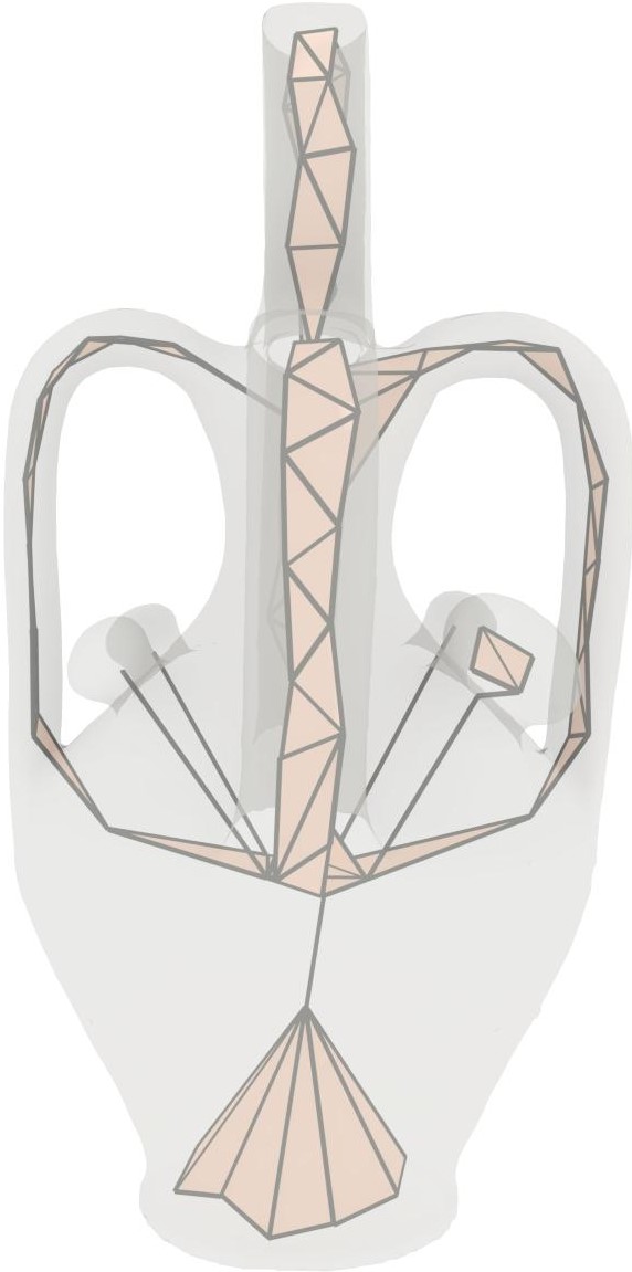
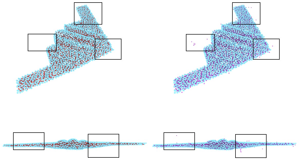
It is worth noting that Q-MAT heavily relies on the quality of the input mesh and the initial Voronoi diagram to compute the medial axis skeleton. In contrast, our method does not have this restriction. Figure 5 shows a group of examples where Q-MAT yields incorrect structures due to the failure of initialization caused by the poor mesh quality, where our algorithm successfully gives the proper skeletal representation.
Comparison with SAT [MGP10]
One of the main setbacks of this method is that SAT favors a dense representation with a large number of vertices, thus incapable of generating a simple and compact skeleton for shape abstraction. In this comparison with SAT, we test different values of its scaling factor, i.e., , and . The qualitative and quantitative comparison results are shown in Figure 7. On the one hand, despite high accuracy yielded by SAT using smaller , its representation has a large number of vertices (Figure 7 (a-c)). This redundant representation is not amenable for various applications that require skeleton to be simple and expressive, e.g., shape matching and retrieval [SSGD03], skeletal animation [MLT88], animated mesh approximation [YYG18, TGBE16], etc. On the other hand, using a larger for a higher abstraction level destroys the shape structure and causes large approximation errors. Our method, on the contrary, provides trade-offs across fidelity, efficiency and compression abilities.
Both Q-MAT and SAT can only excel at handling watertight surface meshes. As aforementioned, the surface mesh input allows robust computation of the Voronoi diagram, which offers good structural information from both inside and outside. Instead, generating skeletal representations for point clouds is more challenging and beyond the capacity of these methods. Our method is able to take unstructured point sets as input and generate skeletal representations of which connected structures are recovered. We will evaluate this property of our method in the following section.
5.2 Coverage Axis from Point Cloud Input
For point cloud input, we compare with two closely relevant methods: Deep Point Consolidation (DPC) [WHG*15] and Point2Skeleton [LLL*21], given that these two methods can also predict MAT-based skeletons directly from point clouds. Note Point2Skeleton is a deep learning-based method that requires training from a large amount of data.
![[Uncaptioned image]](https://cdn.awesomepapers.org/papers/49feae21-a757-4b7a-a5b1-e56762f1f6f4/vase1.1.jpg)
![[Uncaptioned image]](https://cdn.awesomepapers.org/papers/49feae21-a757-4b7a-a5b1-e56762f1f6f4/hand1.1.jpg)
![[Uncaptioned image]](https://cdn.awesomepapers.org/papers/49feae21-a757-4b7a-a5b1-e56762f1f6f4/fertility1.1.jpg)
![[Uncaptioned image]](https://cdn.awesomepapers.org/papers/49feae21-a757-4b7a-a5b1-e56762f1f6f4/dog1.1.jpg)
![[Uncaptioned image]](https://cdn.awesomepapers.org/papers/49feae21-a757-4b7a-a5b1-e56762f1f6f4/Crabs1.1.jpg)
![[Uncaptioned image]](https://cdn.awesomepapers.org/papers/49feae21-a757-4b7a-a5b1-e56762f1f6f4/vase1.5.jpg)
![[Uncaptioned image]](https://cdn.awesomepapers.org/papers/49feae21-a757-4b7a-a5b1-e56762f1f6f4/hand1.5.jpg)
![[Uncaptioned image]](https://cdn.awesomepapers.org/papers/49feae21-a757-4b7a-a5b1-e56762f1f6f4/fertility1.5.jpg)
![[Uncaptioned image]](https://cdn.awesomepapers.org/papers/49feae21-a757-4b7a-a5b1-e56762f1f6f4/dog1.5.jpg)
![[Uncaptioned image]](https://cdn.awesomepapers.org/papers/49feae21-a757-4b7a-a5b1-e56762f1f6f4/Crabs1.5.jpg)
![[Uncaptioned image]](https://cdn.awesomepapers.org/papers/49feae21-a757-4b7a-a5b1-e56762f1f6f4/vase2.jpg)
![[Uncaptioned image]](https://cdn.awesomepapers.org/papers/49feae21-a757-4b7a-a5b1-e56762f1f6f4/hand2.jpg)
![[Uncaptioned image]](https://cdn.awesomepapers.org/papers/49feae21-a757-4b7a-a5b1-e56762f1f6f4/fertility2.jpg)
![[Uncaptioned image]](https://cdn.awesomepapers.org/papers/49feae21-a757-4b7a-a5b1-e56762f1f6f4/dog2.jpg)
![[Uncaptioned image]](https://cdn.awesomepapers.org/papers/49feae21-a757-4b7a-a5b1-e56762f1f6f4/Crabs2.jpg)
offset=
(a)
(b)
(c)
(d)
Comparison with Deep Point Consolidation [WHG*15]
As shown in Figure 6 and Table 2, this method can only produce unstructured inner points without connections. Although the skeletons generated by DPC have denser points, the reconstruction results still exhibit large errors. Even worse, the reconstructed topologies by deep point consolidation are usually inconsistent with the original input. In contrast, our reconstruction results reach better approximation accuracy with respect to the original geometry using fewer skeletal points.
Comparison with Point2Skeleton [LLL*21]
More recently, using deep neural networks to predict skeletal representations from point clouds is beginning to be studied. Point2Skeleton [LLL*21] is a representative approach that directly learns skeletal representations from point clouds based on the MAT in an unsupervised manner. We use their pre-trained network on a large quantity of data for comparison.
| Model | P2S | DPC | Coverage Axis | |||
| Ant-2 | 2.350% | |||||
| Bottle | 2.752% | |||||
| Chair-2 | 2.890% | |||||
| Dog | 2.174% | |||||
| Dolphin | 1.971% | |||||
| Fertility | 3.428% | |||||
| Guitar | 2.032% | |||||
| Hand-1 | 3.441% | |||||
| Human-2 | 1.667% | |||||
| Kitten | 3.450% | |||||
| Snake | 1.309% | |||||
| Average | - | - | - | 2.515% | ||
-
1
The number of skeleton points.
-
2
Two-sided HD between original surface and reconstruction.
Figure 6 as well as Table 2 show the comparison results. Note that Guitar and Chair-2 are from ShapeNet [CFG*15] dataset which is used for training Point2Skeleton. First, an obvious problem with Point2Skeleton is their limited generalization abilities; despite being trained on numerous data, it still generates unsatisfactory results for unseen shapes. Furthermore, it performs poorly on models with higher topology complexity, e.g., input with more than genus one. Also, the neural network shows incapability for capturing the properties of geometric transforms, such as the centrality of skeletal points. Conversely, our approach is robust to various shapes and can produce high-quality skeletal representations that have accurate geometries and faithful structures.
6 Discussions
In this section, in order to provide more insights and have better understandings of the proposed algorithm, we further give an in-depth analysis of some interesting properties of the Coverage Axis.
6.1 Centrality and Random Initialization
A good skeleton requires each skeletal point to be located at the center of its corresponding local geometry. Our method is able to effectively select the local centers for generating the skeletal representation. This property also enables our algorithm to handle randomly generated inner points instead of relying on computing the strictly defined Voronoi diagram as an input. In this section, we elaborate on this centrality property of our point selection strategy.
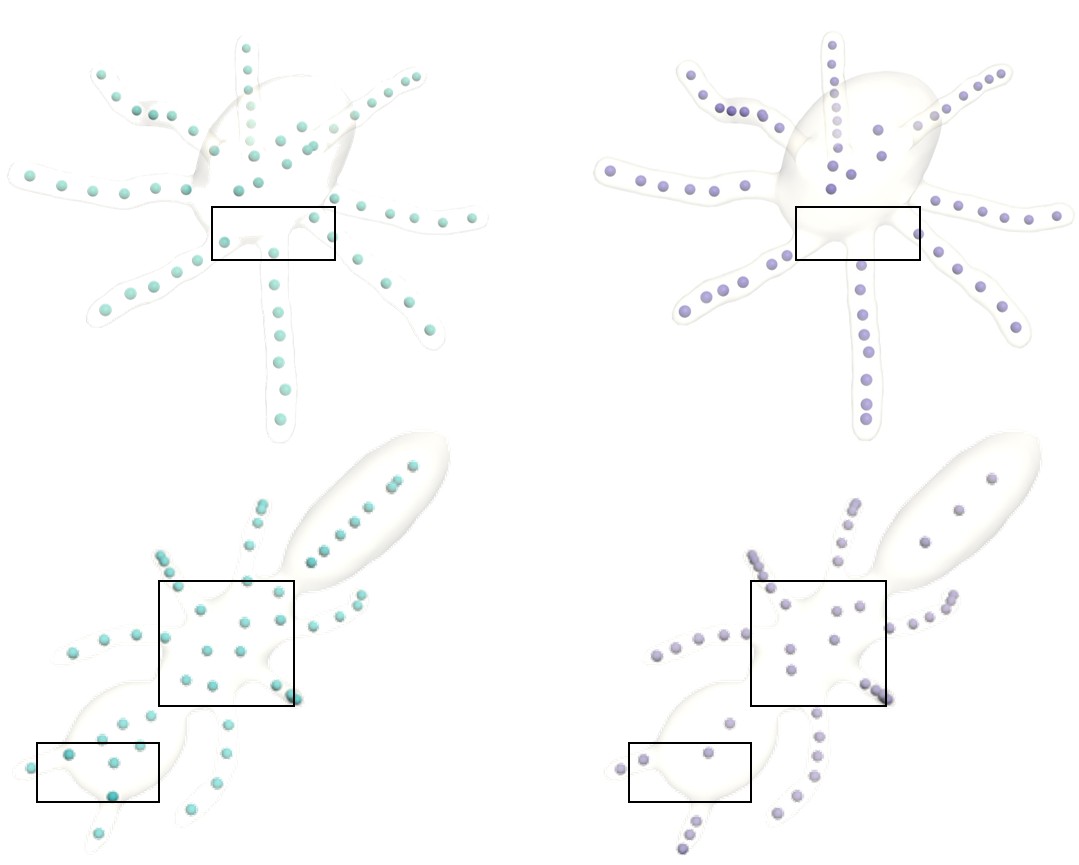
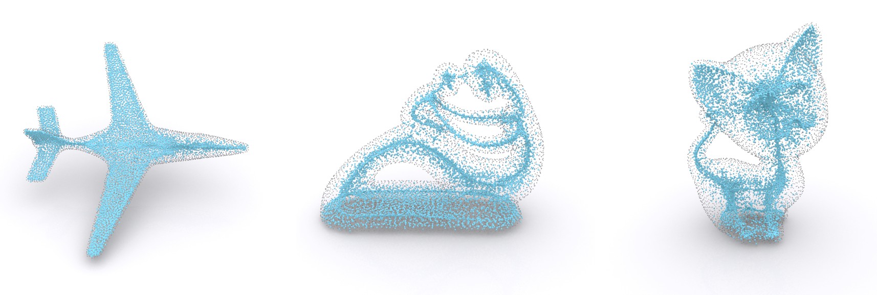
We first generate the point candidates by randomly sampling inside the shape and then applying our point selection algorithm introduced in Sec 4.2. The number of randomly generated inner points is , and the offset is set to . A selection of results from these randomly generated points are shown in Figure 8. Thanks to the idea of optimal set coverage, it can be observed that the selected points are located at the centers of local geometry, even if the initial points are derived by random sampling. An evaluation of the influence of different randomly generated candidate inner point numbers for centrality is given in Figure 9. We find different numbers of candidate inner points do not show a large influence on the centrality.
In the following, we give an analysis of the rationale of the centrality property of our algorithm. Recall in Eq. 2, the constraint of the optimization is that the union of dilated balls needs to cover the sampled surface points. As explained in Sec. 6.4, the dilated radius should not deviate too much from the original radius, which means . Consider a local shape shown in Figure 10. The coverage goal of one candidate point is defined by its farthest distance to the local geometry, e.g., , given that all the surface samples are covered only if the farthest sample is covered. According to the definition of inner balls, the coverage ability is determined by its radius (note that we have ), which is actually the distance to the nearest surface samples of the local geometry.
The goal of finding the minimum number of dilated balls to cover all surface samples can be viewed as selecting those points with the most powerful coverage ability (cover all the target samples). That to say, its radius should be as equal as possible to the distance to farthest point so that we have which satisfies the coverage constraint. Those balls whose radii are close to the distance to the farthest point that needs to be covered will be preferred during optimization. Note that is consistent with the definition of the medial axis, which is intrinsically a set of centers of maximally inscribed spheres. In this case, the inner point is preferred for the local geometry coverage since . Note that we always have . Finally, as shown in Figure 10, is a better approximation than of skeleton point and will be selected by our strategy.
6.2 Robustness to Noise
We evaluate the robustness of our method to surface noise. We compare with Q-MAT [LWS*15], which has the state-of-the-art performance in terms of approximation accuracy and goodness of structure (i.e., compactness and shape awareness). The number of vertices of the skeletal points are set the same for both methods. As shown in Figure 11, given noisy input, our method can still preserve the main features and achieve relatively high-precision shape approximation with a compact representation. The robustness mainly owes to the ball dilation strategy as well as the formulation based on global coverage. The dilated balls cover the insignificant details cause by local perturbations, while the overall coverage formulation gives a high-level optimization rather than focusing on local details. In contrast, Q-MAT [LWS*15], which uses step-by-step edge collapse based on local errors, cannot capture the fine details when the input surface has great noise.
6.3 Dilation Strategy
(a)
(b)
As aforementioned, the relationship between inner points and surface is built by the coverage, which is achieved by dilating the medial radius. There are two typical ways for inner ball dilation. One is by adding a specified value to the radius of each ball. The other is to scale the ball by multiplying the radius by a factor . We now discuss the effect of these two dilation strategies. To facilitate the discussion, we refer to the first way as offset and the second as scaling.
We take the model Octopus and Ant-3 as examples. Let and denote the original medial radius and dilated medial radius respectively. For the offset manner, we set where , while for the scaling manner, we set with .
As shown in Figure 12, the offset manner tends to generate selected points that are distributed more evenly, while the scaling manner can distinguish parts that have different radii, which leads to relatively large gap around the joints of different parts (as shown in the box region). The reason behind this is, adding a constant value is independent of the original radius, but the scaling makes the larger ball dilate more and control more area, which results in part differentiation.
6.4 Parameter Analysis
Dilation Factor
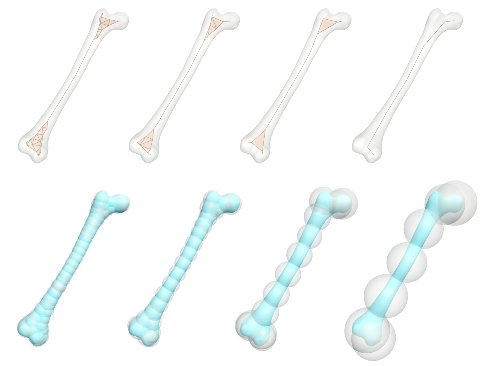
The dilation factor is an important parameter that controls the simplicity of the output skeleton. In the following, we discuss the effect of different values of the parameter . We use the Femur model as an example for demonstration, whose results are shown in Figure 13.
Obviously, a larger radius enables a ball to cover more surface points, which allows the algorithm to use fewer inner balls to cover the whole geometry. Therefore, a larger will lead to a higher simplified skeletal representation that captures less geometric details. Actually, the premise that we use surface information for simplification is that the envelope formed by dilated balls should not deviate significantly from the geometry of the input shape. On the one hand, we recommend not setting an excessively large , as this leads to the over-dilated balls of which union are inconsistent with the original shape structure. On the other hand, being too small is also discouraged because it runs counter to the simplicity and compactness, which are related requirements for a skeletal representation. In this paper, we always set for our experiments.
(a)
(b)
(c)
(d)
Surface points and inner points.
To investigate the influence of the number of surface points and candidate inner points (note it is determined by , i.e., the number of samples to compute Voronoi diagram) on the algorithm performance, we conduct comprehensive experiments. We find that these two parameters do not show a significant influence on the selected point number and the quality of the resulting medial mesh. See more details in Appendix C. However, it has more effect on the time efficiency, for which a detailed analysis is given in Sec. 6.5.
6.5 Time Efficiency
We further discuss the time efficiency of our point selection strategy. The statistics is summarized in Table 3. We use Mixed-integer linear programming (MILP) solver in MATLAB (MathWorks 2021) on the platform explained in Sec 5.
As aforementioned, the experiments are conducted with mesh input using surface point samples, candidate inner points generated by surface samples. The dilation offset is set to . It can be viewed from Table 3 that the point selection only takes a few seconds for most shapes. For some cases, the complexity of the searching space of the Set Coverage problem may increase, which leads to one to two minutes of running time. The average running time for all the samples is s.
| Model | Time (s) | Model | Time (s) | ||||
| Ant-1 | Hand-1 | ||||||
| Armadillo | Hand-2 | ||||||
| Kitten | Human-1 | ||||||
| Bunny | Horse | ||||||
| Crab | Octopus-1 | ||||||
| Camel | Octopus-2 | ||||||
| Dog | Pig | ||||||
| Dolphin | Pliers | ||||||
| Duck | Snake | ||||||
| Elephant | Spider | ||||||
| Eight | Spectacle | ||||||
| Fish | Bear | ||||||
| Fertility | Vase | ||||||
| Femur | Venus | ||||||
| Average |
| Model | Mesh Input | Point Cloud Input | ||||
| Q-MAT | SAT | Ours | DPC | P2S | Ours | |
| Ant-1 | ||||||
| Bunny | ||||||
| Horse | ||||||
| Pig | ||||||
| Venus | ||||||
Table 3 also reveals the difference in running time for various shapes, where the difference is because the complexity of the solution space in SCP varies for different geometries. Generally, solving for the coverage of plate-like geometries is more complex than tube-like ones, since the plate-like models have more eligible candidates that satisfy the coverage constraints, which leads to a larger search space during optimization. Since many shapes consist of both tube-like and plate-like structures, there is a variation in running times. We further report running time comparison in Table 4.
SCP is a known NP-Hard problem [Har82] and its running time complexity is where and are the number of candidate inner points and surface points, respectively. To investigate the influence of and on running time efficiency and the resulting number of selected skeletal points , we conduct additional experiments of which results are summarized in Table 1 and Table 2 respectively. We adopt the Octopus-1 model for evaluation. We fix in Table 1 and in Table 2. From the results, both and do not show a significant influence on the selected vertex number. However, has a larger impact on the running time, while shows less effect, which is consistent with the aforementioned analysis of time complexity.
| Time (s) | ||
| Time (s) | |||
| Model | Ant-2 | FEMUR | Hand-2 | Fertility | ||||||||||||
| Offset | ||||||||||||||||
| Selected points | ||||||||||||||||
| Time (s) | ||||||||||||||||
| Scaling | ||||||||||||||||
| Selected points | ||||||||||||||||
| Time (s) | ||||||||||||||||
To evaluate the time efficiency for different algorithm settings, we conduct an additional experiment where the initial candidate points are generated by random sampling. Here, we randomly sample points inside a shape and test the time efficiency using two different dilation strategies and different dilation factors. The results are given in Table 7. It can be observed the running time is stable in different configurations.
7 Additional Features of Coverage Axis
In this section, we analyze some of the other interesting features of our method, including the ability to handle large models and the flexibility of user-specified point control.
7.1 Divide and Conquer Strategy for Large Models
Since the set coverage problem is NP-hard, the action space grows exponentially with respect to the number of surface points. Fortunately, an interesting feature of the proposed method is the flexibility in handling large complex models. The overall insights lie in the combination of divide and conquer strategy and our set coverage formulation. In this case, we take a mesh model with Voronoi initialization for explanation.
The first step is decomposing a mesh into smaller and meaningful sub-meshes with some existing methods, e.g., [YL21, HHF*19]. Then we have surface samples divided into several subsets where is the number of surface components. According to the correspondence between the vertices on the inside Voronoi diagram and the surface samples, we partition the inside Voronoi diagram into accordingly. For each component , with surface samples and inner point candidates , we solve the SCP and obtain the selection result embedded on the sub-Voronoi diagram. This process reduces the size of the problem and speeds up our algorithm by divide and conquer.
Finally, we merge each Voronoi diagram as well as the selected points. Then, we have all the selected points embedded on the original inside Voronoi diagram so that the model’s simplification can be achieved by removing redundant components as we described in Sec. 4.3. We demonstrate the results in Figure 14 (a-b). Note that the complex model is with surface samples which are further used for generating candidate inner points.
7.2 User-specified Point Control
Our method allows users to specify the ignorable surface parts that can be neglected. To indicate the ignorable surface points, the constraint in Eq 2 are reformulated as , where the corresponding values for the ignorable surface points in are set to and the others to . In this way, the optimization tends to remove the skeletal points in the specified parts to favor parsimony. Users can also directly indicate if a skeletal point should be preserved or removed, for which we just simply set the corresponding values in to 0 or 1 after the point selection.
8 Limitations
(a)
(b)
In this section, we discuss the limitations of our method. First, the number of selected points is related to the dilation parameter which leads to a difficulty in explicit control of the number of vertices of a skeleton. In particular, when inner balls are excessively dilated, the topology of the input surface tends to be destroyed by the coverage. See Figure 15 (a). Another limitation lies in the difficulty in preserving approximation accuracy when computing extremely decimated representations (lower vertices number in the skeleton). As shown in Figure 16, Q-MAT [LWS*15] shows a better control of the reconstruction error than ours, as the number of target skeletal points decreases. This is because Coverage Axis relies on much larger dilation factors for computing highly decimated results, which brings difficulty in preserving the local geometry. Detailed statistics can be found in Appendix D.
Our method usually suffers from a relatively high computational cost when given a large number of surface points to be covered. To alleviate this, we demonstrate a potential approach in designing a divide and conquer strategy based on geometric clues to achieve acceleration. In addition, for the point cloud input, especially the thin flat models, it remains an open problem to clearly distinguish between inner and outside volume. Therefore, for this kind of input, it is extremely challenging to generate legitimate candidate points that are located inside the shape, which can result in failure cases during point selection (Figure 15 (b)).
9 Conclusion
In this paper, we propose a novel, simple, yet effective formulation named Coverage Axis for 3D shape skeletonization of both meshes and point clouds. Inspired by the set cover problem (SCP), our goal is to cover all the surface points using as few inside medial balls as possible. Compared with previous methods, our approach shows a set of appealing properties including its simple formulation, high-level abstraction, robustness to noise, flexibility to handle various cases, and so on. Comprehensive experiments verify the aforementioned claims. In the future, we believe Coverage Axis, as a tool for encoding shapes, has a large potential value in various applications including shape abstraction, shape segmentation, simulation as well as animation, etc. Another point worth noting is the combination of Coverage Axis and learning techniques to improve the work of shape analysis and processing, such as 3D object detection, shape classification, automatic blending and so on.
References
- [ABE09] Dominique Attali, Jean-Daniel Boissonnat and Herbert Edelsbrunner “Stability and computation of medial axes-a state-of-the-art report” In Mathematical foundations of scientific visualization, computer graphics, and massive data exploration Springer, 2009, pp. 109–125
- [ACK01] Nina Amenta, Sunghee Choi and Ravi Krishna Kolluri “The power crust” In Proceedings of the sixth ACM symposium on Solid modeling and applications, 2001, pp. 249–266
- [AM96] Dominique Attali and Annick Montanvert “Modeling noise for a better simplification of skeletons” In Proceedings of 3rd IEEE International Conference on Image Processing 3, 1996, pp. 13–16 IEEE
- [And09] Daniel Cohen-Or Andrea Tagliasacchi “Curve skeleton extraction from incomplete point cloud” In ACM Transactions on Graphics (Proc. SIGGRAPH) 28.3, 2009, pp. 71:1–71:9
- [ATC*08] Oscar Kin-Chung Au et al. “Skeleton extraction by mesh contraction” In ACM transactions on graphics (TOG) 27.3 ACM New York, NY, USA, 2008, pp. 1–10
- [Aur87] Franz Aurenhammer “Power diagrams: properties, algorithms and applications” In SIAM Journal on Computing 16.1 SIAM, 1987, pp. 78–96
- [BDS*18] Gavin Barill et al. “Fast Winding Numbers for Soups and Clouds” In ACM Transactions on Graphics, 2018
- [Blu*67] Harry Blum “A transformation for extracting new descriptors of shape” MIT press Cambridge, MA, 1967
- [BP07] Ilya Baran and Jovan Popović “Automatic rigging and animation of 3d characters” In ACM Transactions on graphics (TOG) 26.3 ACM New York, NY, USA, 2007, pp. 72–es
- [CCT11] John Chaussard, Michel Couprie and Hugues Talbot “Robust skeletonization using the discrete -medial axis” In Pattern Recognition Letters 32.9 Elsevier, 2011, pp. 1384–1394
- [CFG*15] Angel X Chang et al. “Shapenet: An information-rich 3d model repository” In arXiv preprint arXiv:1512.03012, 2015
- [CL05] Frédéric Chazal and André Lieutier “The “-medial axis”” In Graphical Models 67.4 Elsevier, 2005, pp. 304–331
- [CTO*10] Junjie Cao et al. “Point cloud skeletons via laplacian based contraction” In 2010 Shape Modeling International Conference, 2010, pp. 187–197 IEEE
- [CZC*20] Jingliang Cheng et al. “Skeletonization via dual of shape segmentation” In Computer Aided Geometric Design 80 Elsevier, 2020, pp. 101856
- [DEGN98] Tamal K Dey, Herbert Edelsbrunner, Sumanta Guha and Dmitry V Nekhayev “Topology preserving edge contraction” In Publ. Inst. Math.(Beograd)(NS, 1998 Citeseer
- [DRS10] Jesús De Loera, Jörg Rambau and Francisco Santos “Triangulations: Structures for algorithms and applications” Springer Science & Business Media, 2010
- [DS06] Tamal K Dey and Jian Sun “Defining and computing curve-skeletons with medial geodesic function” In Symposium on geometry processing 6, 2006, pp. 143–152
- [DXX*20] Zhiyang Dou et al. “Top-down shape abstraction based on greedy pole selection” In IEEE Transactions on Visualization and Computer Graphics IEEE, 2020
- [DZ02] Tamal K Dey and Wulue Zhao “Approximate medial axis as a Voronoi subcomplex” In Proceedings of the seventh ACM symposium on Solid modeling and applications, 2002, pp. 356–366
- [FLM03] Mark Foskey, Ming C Lin and Dinesh Manocha “Efficient computation of a simplified medial axis” In J. Comput. Inf. Sci. Eng. 3.4, 2003, pp. 274–284
- [FTB13] Noura Faraj, Jean-Marc Thiery and Tamy Boubekeur “Progressive medial axis filtration” In SIGGRAPH Asia 2013 Technical Briefs, 2013, pp. 1–4
- [GH97] Michael Garland and Paul S Heckbert “Surface simplification using quadric error metrics” In Proceedings of the 24th annual conference on Computer graphics and interactive techniques, 1997, pp. 209–216
- [GMPW09] Joachim Giesen, Balint Miklos, Mark Pauly and Camille Wormser “The scale axis transform” In Proceedings of the twenty-fifth annual symposium on Computational geometry, 2009, pp. 106–115
- [Har82] Juris Hartmanis “Computers and intractability: a guide to the theory of np-completeness (michael r. garey and david s. johnson)” In Siam Review 24.1 Society for IndustrialApplied Mathematics, 1982, pp. 90
- [HHF*19] Rana Hanocka et al. “MeshCNN: A network with an edge” In ACM Transactions on Graphics (TOG) 38.4 ACM New York, NY, USA, 2019, pp. 1–12
- [HWC*13] Hui Huang et al. “L1-medial skeleton of point cloud.” In ACM Trans. Graph. 32.4, 2013, pp. 65–1
- [HWG*13] Hui Huang et al. “Edge-aware point set resampling” In ACM transactions on graphics (TOG) 32.1 ACM New York, NY, USA, 2013, pp. 1–12
- [LCLT07] Yaron Lipman, Daniel Cohen-Or, David Levin and Hillel Tal-Ezer “Parameterization-free projection for geometry reconstruction” In ACM Transactions on Graphics (TOG) 26.3 ACM New York, NY, USA, 2007, pp. 22–es
- [LGS12] Marco Livesu, Fabio Guggeri and Riccardo Scateni “Reconstructing the curve-skeletons of 3d shapes using the visual hull” In IEEE transactions on visualization and computer graphics 18.11 IEEE, 2012, pp. 1891–1901
- [LLL*20] Cheng Lin et al. “SEG-MAT: 3D shape segmentation using medial axis transform” In IEEE Transactions on Visualization and Computer Graphics IEEE, 2020
- [LLL*21] Cheng Lin et al. “Point2Skeleton: Learning skeletal representations from point clouds” In Proceedings of the IEEE/CVF Conference on Computer Vision and Pattern Recognition, 2021, pp. 4277–4286
- [LWS*15] Pan Li et al. “Q-MAT: Computing medial axis transform by quadratic error minimization” In ACM Transactions on Graphics (TOG) 35.1 ACM New York, NY, USA, 2015, pp. 1–16
- [MGP10] Balint Miklos, Joachim Giesen and Mark Pauly “Discrete scale axis representations for 3D geometry” In ACM SIGGRAPH 2010 papers, 2010, pp. 1–10
- [MLM16] Romain Marie, Ouiddad Labbani-Igbida and El Mustapha Mouaddib “The delta medial axis: a fast and robust algorithm for filtered skeleton extraction” In Pattern Recognition 56 Elsevier, 2016, pp. 26–39
- [MLT88] Nadia Magnenat-Thalmann, Richard Laperrire and Daniel Thalmann “Joint-dependent local deformations for hand animation and object grasping” In In Proceedings on Graphics interface’88, 1988 Citeseer
- [MWO03] Wan-Chun Ma, Fu-Che Wu and Ming Ouhyoung “Skeleton extraction of 3D objects with radial basis functions” In 2003 Shape Modeling International., 2003, pp. 207–215 IEEE
- [NBPF11] Mattia Natali, Silvia Biasotti, Giuseppe Patanè and Bianca Falcidieno “Graph-based representations of point clouds” In Graphical Models 73.5 Elsevier, 2011, pp. 151–164
- [RAV*19] Daniel Rebain et al. “LSMAT Least squares medial axis transform” In Computer Graphics Forum 38.6, 2019, pp. 5–18 Wiley Online Library
- [RLS*21] Daniel Rebain et al. “Deep medial fields” In arXiv preprint arXiv:2106.03804, 2021
- [SBH*11] Wei Shen et al. “Skeleton growing and pruning with bending potential ratio” In Pattern Recognition 44.2 Elsevier, 2011, pp. 196–209
- [SCYW13] Feng Sun, Yi-King Choi, Yizhou Yu and Wenping Wang “Medial meshes for volume approximation” In arXiv preprint arXiv:1308.3917, 2013
- [SFC*11] Jamie Shotton et al. “Real-time human pose recognition in parts from single depth images” In CVPR 2011, 2011, pp. 1297–1304 Ieee
- [SFM07] Avneesh Sud, Mark Foskey and Dinesh Manocha “Homotopy-preserving medial axis simplification” In International Journal of Computational Geometry & Applications 17.05 World Scientific, 2007, pp. 423–451
- [SKS11] Svetlana Stolpner, Paul Kry and Kaleem Siddiqi “Medial spheres for shape approximation” In IEEE transactions on pattern analysis and machine intelligence 34.6 IEEE, 2011, pp. 1234–1240
- [SLSK07] Andrei Sharf, Thomas Lewiner, Ariel Shamir and Leif Kobbelt “On-the-fly Curve-skeleton Computation for 3D Shapes” In Computer Graphics Forum 26.3, 2007, pp. 323–328 Wiley Online Library
- [SSGD03] Hari Sundar, Deborah Silver, Nikhil Gagvani and Sven Dickinson “Skeleton based shape matching and retrieval” In 2003 Shape Modeling International., 2003, pp. 130–139 IEEE
- [TAOZ12] Andrea Tagliasacchi, Ibraheem Alhashim, Matt Olson and Hao Zhang “Mean curvature skeletons” In Computer Graphics Forum 31.5, 2012, pp. 1735–1744 Wiley Online Library
- [TDS*16] Andrea Tagliasacchi et al. “3d skeletons: A state-of-the-art report” In Computer Graphics Forum 35.2, 2016, pp. 573–597 Wiley Online Library
- [TGB13] Jean-Marc Thiery, Émilie Guy and Tamy Boubekeur “Sphere-meshes: Shape approximation using spherical quadric error metrics” In ACM Transactions on Graphics (TOG) 32.6 ACM New York, NY, USA, 2013, pp. 1–12
- [TGBE16] Jean-Marc Thiery, Émilie Guy, Tamy Boubekeur and Elmar Eisemann “Animated mesh approximation with sphere-meshes” In ACM Transactions on Graphics (TOG) 35.3 ACM New York, NY, USA, 2016, pp. 1–13
- [THP*19] Jiapeng Tang et al. “A skeleton-bridged deep learning approach for generating meshes of complex topologies from single rgb images” In Proceedings of the IEEE/CVF Conference on Computer Vision and Pattern Recognition, 2019, pp. 4541–4550
- [WHG*15] Shihao Wu et al. “Deep points consolidation” In ACM Transactions on Graphics (ToG) 34.6 ACM New York, NY, USA, 2015, pp. 1–13
- [XZKS19] Zhan Xu, Yang Zhou, Evangelos Kalogerakis and Karan Singh “Predicting animation skeletons for 3d articulated models via volumetric nets” In 2019 International Conference on 3D Vision (3DV), 2019, pp. 298–307 IEEE
- [YL21] Ilker O. Yaz and Sébastien Loriot “Triangulated Surface Mesh Segmentation” In CGAL User and Reference Manual CGAL Editorial Board, 2021 URL: https://doc.cgal.org/5.3/Manual/packages.html#PkgSurfaceMeshSegmentation
- [YLJ18] Yajie Yan, David Letscher and Tao Ju “Voxel Cores: Efficient, robust, and provably good approximation of 3d medial axes” In ACM Transactions on Graphics (TOG) 37.4 ACM New York, NY, USA, 2018, pp. 1–13
- [YRL*21] Yiding Yang et al. “Learning dynamics via graph neural networks for human pose estimation and tracking” In Proceedings of the IEEE/CVF Conference on Computer Vision and Pattern Recognition, 2021, pp. 8074–8084
- [YSC*16] Yajie Yan et al. “Erosion thickness on medial axes of 3D shapes” In ACM Transactions on Graphics (TOG) 35.4 ACM New York, NY, USA, 2016, pp. 1–12
- [YYG18] Baorong Yang, Junfeng Yao and Xiaohu Guo “DMAT: Deformable medial axis transform for animated mesh approximation” In Computer Graphics Forum 37.7, 2018, pp. 301–311 Wiley Online Library
- [YYW*20] Baorong Yang et al. “P2MAT-Net: Learning medial axis transform from sparse point clouds” In Computer Aided Geometric Design 80 Elsevier, 2020, pp. 101874
cgal:tf-ssd-21b
Appendix A Inner Points Labeling for Point Cloud with Normals.
Our point selection strategy does not rely on mesh connection; it is able to handle more generalized inputs such as polygon soups, point clouds as long as candidate inner points can be identified inside the volume. Given a point cloud input, in this paper, we generate and label candidate inner points by utilizing normal vectors of the point cloud. Recall that we first compute its Delaunay triangulation which is the dual of the Voronoi diagram w.r.t. the input point cloud. Consider a Voronoi vertex and the vertices of its dual tetrahedron and . The candidate is considered as an inner point only if we have , . Here is the input normal of and is dot product. A detailed 2D example is given in Figure 1.
After the initial labeling, we further apply filtering by clustering to those labeled inner points. For each inner point, we count the number of its neighbors within among the top nearest neighbors by K-neighbor searching [cgal:tf-ssd-21b]. If the result is less than , the point is considered an outlier and is discarded. A result of the UFO model as an example is shown in Figure 2. Some labeling results are given in Figure 3.
(a)
(b)
![[Uncaptioned image]](https://cdn.awesomepapers.org/papers/49feae21-a757-4b7a-a5b1-e56762f1f6f4/fig_poles2.jpg)
Besides, we also conduct an experiment taking inside poles [ACK01] (the inside Voronoi vertex with the furthest distance to the seed of the cell) instead of all Voronoi vertices enclosed by the surface as candidates. We find there is no significant difference in point selection results.
Appendix B Details of Connection Establishment.
B.1 Mesh Input
Recall that for a mesh input, we take the whole subset of Voronoi structure inside the model generated by surface samples () as the original inner point candidates . After selecting inner points based on set coverage, we build up the connection structure. For the Voronoi initialization style, all selected points are embedded on the Voronoi diagram. We further remove all redundant points and edges to achieve the simplification by edge collapse using quadric error metric (QEM) [FTB13] same as [LWS*15].
After that, we adopt LOP [DRS10] algorithm to adjust the mesh tessellations as long as the increase of the local approximation error caused by the flipping operation is less than . The local approximation error is measured by the Hausdorff distance from the covered surface to candidate local reconstructed surfaces (the envelope of two candidate triangulation.), a.k.a., one-sided Hausdorff distance. Note that we first unstitch each face patch based on non-manifold edges before performing LOP.
B.2 Point Cloud Input
In order to suppress over-connection, we up-sample on the point cloud with normals following [HWG*13], leading to surface samples. These points are treated as surface points in RT during connection establishment. The effect of point cloud up-sampling is demonstrated in Figure 4.
Appendix C Parameter Analysis on Surface points and Candidate Inner Points.
We conduct comprehensive experiments on the number of surface points and candidate inner points (note it is determined by , which is the number of samples to compute the Voronoi diagram) for the algorithm performance. Detailed results including approximation error are summarized in Table 1 and Table 2, respectively. In Table 1, we fix and in Table 2, we always set . Same as the main paper, we use to denote the number of skeletal points, to denote the HD from surface to reconstruction, to denote the HD from reconstruction to surface, and to represent two-sided HD. We find both and do not show a large influence on the selected point number as well as the approximation error. However, as we mentioned in the main paper, the two factors, especially the number of surface samples , have more effect on the time efficiency.
| Time (s) | |||||
| Time (s) | ||||||
Appendix D Comparison with Q-MAT for Highly Decimated MAT Computation.
| Offset | Q-MAT | Coverage Axis | |||||
The quantitative comparison of surface reconstruction by highly decimated medial surfaces between Q-MAT and Coverage Axis is shown in Table 3.