This paper was converted on www.awesomepapers.org from LaTeX by an anonymous user.
Want to know more? Visit the Converter page.

Critical behavior of two-choice rules,
a class of Achlioptas processes

Braden Hoagland and Rick Durrett
Dept of Math, P.O. Box 90320, Duke University, Durham NC 27708
A version of this paper was Braden’s senior thesis at Duke. He now works at IMC Trading in Chicago. RD was partially spported by NSF grants DMS 1809967 and 2153429 from the probability program
Abstract

Achlioptas processes are a class of dynamically grown random graphs where on each step several edges are chosen at random but only one is added. The sum rule, product rule, and bounded size rules have been extensively studied. Here we introduce a new collection of rules called two-choice rules. In these systems one first pick mm vertices at random from the graph and chooses a vertex vv according to some rule based on their cluster sizes. The procedure is then repeated with a second independent sample to pick a vertex vv^{\prime} and we add an edge from vv and vv^{\prime}. These systems are tractable because the cluster size distribution satisfies an analog of the Smoluchowski equation. We study the critical exponents associated with the phase transitions in five of these models. In contrast to the situation for dd-dimensional percolation we show that all of the critical exponents can be computed if we know β\beta, the exponent associated with the size of the giant component. When β=1\beta=1 all the critical exponents are the same as for the Erdös-Rényi graph.

1 Summary of results

We study the phase transitions of a class of dynamically grown graphs that we call two-choice rules. We start with a graph with nn vertices and no edges. In general, on each step we first pick mm vertices v1,,vmv_{1},\ldots,v_{m} at random and choose one, vv, according to some rule. We then pick a second set of mm vertices v1,,vmv^{\prime}_{1},\ldots,v^{\prime}_{m}, choose one of them, vv^{\prime}, according to the same rule, and then add (v,v)(v,v^{\prime}) to the graph.

The Erdös-Rényi graph is the degenerate m=1m=1 case of our system: on each step we pick an edge at random and add it to the graph. To be able to take the limit as nn\to\infty we say that graph with mm edges occurs at time t=2m/nt=2m/n, so that in the limit as nn\to\infty the mean degree of vertices at time tt is tt. In the case of Erdös-Rényi this means the threshold for the existence of a giant component is tc=1t_{c}=1. In many papers the graph with mm edges occurs at time t=m/nt=m/n so in the case of Erdös-Rényi this means the threshold for the existence of a giant component is tc=1t_{c}=1.

If we let κi\kappa_{i} be the size of the cluster containing viv_{i} then in three of the rules we consider we choose a vertex (i) with the smallest κi\kappa_{i}, (ii) with the largest κi\kappa_{i}, or (iii)with the median κi\kappa_{i} (assuming mm is odd). In our fourth system called the Bohman-Frieze vertex rule, we choose an isolated vertex (i.e., κi=1\kappa_{i}=1) if there is one in the set, otherwise choose at random from the set. In our fifth example, the alternative edge rule [11], a vertex vv is chosen at random and then a secon vertex vv^{\prime} is chosen accroding to the min rule.

As explained in Section 2 these systems are instances of Achlioptas processes. We now introduce two famous examples. In the sum rule one chooses four vertices v1,v2,v3,v4v_{1},v_{2},v_{3},v_{4} and connect v1,v2v_{1},v_{2} if and only if κ1+κ2κ3+κ4\kappa_{1}+\kappa_{2}\leq\kappa_{3}+\kappa_{4}. In the product rule we connect v1,v2v_{1},v_{2} if and only if κ1κ2κ3κ4\kappa_{1}\cdot\kappa_{2}\leq\kappa_{3}\cdot\kappa_{4}. Achlioptas, D’Souza and Spencer [1] claimed based on simulation that the sum and the product rule had discontinuous phase transitions, but Riordan and Warnkje [22] proved mathematically that the transition was continuous for a very general class of rules. Their proof involved two arguments by contradiction, and hence did not yield much quantitative information about the phase transitions. Here we will study the standard percolation critical exponents for the phase transition of two-choice rules.

1.1 Critical exponents

Let p(s,t)p(s,t) be the probability that a randomly chosen vertex belongs to a cluster of size ss at time tt (in the limit nn\to\infty). Let θ(t)=1sp(s,t)\theta(t)=1-\sum_{s}p(s,t), and χk(t)=sskp(s,t)\chi_{k}(t)=\sum_{s}s^{k}p(s,t) (the value s=s=\infty is excluded from each of the sums). The exponents β\beta, γ\gamma, and Δ\Delta are defined by

θ(t)\displaystyle\theta(t) (ttc)βas ttc\displaystyle\approx(t-t_{c})^{\beta}\qquad\hbox{as $t\downarrow t_{c}$}
χ1(t)\displaystyle\chi_{1}(t) |ttc|γas ttc\displaystyle\approx|t-t_{c}|^{-\gamma}\qquad\hbox{as $t\to t_{c}$}
for k2χk(t)/χk1(t)\displaystyle\hbox{for $k\geq 2$}\quad\chi_{k}(t)/\chi_{k-1}(t) |ttc|Δas ttc\displaystyle\approx|t-t_{c}|^{-\Delta}\qquad\hbox{as $t\to t_{c}$}

In the physics literature the meaning of \approx is not precisely defined. It could be something as weak as

logθ(t)log(ttc)βas ttc\frac{\log\theta(t)}{\log(t-t_{c})}\to\beta\qquad\hbox{as $t\downarrow t_{c}$}

In order to derive relations between exponents we will suppose θ(t)C(ttc)β\theta(t)\sim C(t-t_{c})^{\beta} where a(t)b(t)a(t)\sim b(t) means a(t)/b(t)1a(t)/b(t)\to 1. Our final two exponents concern the behavior near the critical value

p(s,t)s1τf(s|ttc|1/σ)p(s,t)\approx s^{1-\tau}f(s|t-t_{c}|^{1/\sigma}) (1)

where ff is a scaling function.

In Section 5 we will compute the critical exponents for the Erdös-Rényi model,

β=1,γ=1,Δ=2,τ=5/2,σ=1/2\beta=1,\quad\gamma=1,\quad\Delta=2,\quad\tau=5/2,\quad\sigma=1/2 (2)

and show that the scaling relationship (1) holds. These results are well-known. We include them for completeness.

The most significant difference between our critical exponents and those for dd-dimensional percolation is that we do not have a correlation length ξ(p)\xi(p) that gives the spatial size of a typical finite cluster. Thi squantity is often defined in terms of the exponential decay of probability 0 and xx are in the same finite cluster

τf(0,x)=Pp(0x,|𝒞0|<).\tau^{f}(0,x)=P_{p}(0\leftrightarrow x,|{\cal C}_{0}|<\infty).

For example, if e1e_{1} is the first unit vector

ξ(p)=limn1nlogτf(0,ne1)\xi(p)=\lim_{n\to\infty}-\frac{1}{n}\log\tau^{f}(0,ne_{1})

A simpler approach taken by Kesten [18] is to define the correlation length by

ξ(p)=(1χ1(p)y|y|2P(0y;|𝒞0|<))1/2\xi(p)=\left(\frac{1}{\chi_{1}(p)}\sum_{y}|y|^{2}P(0\to y;|{\cal C}_{0}|<\infty)\right)^{1/2}

and the critical exponent ν\nu by ξ(p)|ppc|ν\xi(p)\approx|p-p_{c}|^{-\nu}. Finally on a dd-dimensional graph we have another exponent η\eta called the anomalous dimension

Pcr(0x)|x|2dηP_{cr}(0\to x)\approx|x|^{2-d-\eta}

The percolation critical exponents satisfy the following scaling relationships

β=2νδ+1γ=2νδ1δ+1Δ=2νδδ+1η=4δ\beta=\frac{2\nu}{\delta+1}\qquad\gamma=2\nu\frac{\delta-1}{\delta+1}\qquad\Delta=2\nu\frac{\delta}{\delta+1}\qquad\eta=\frac{4}{\delta} (3)

Kesten [18] established provided that the exponents δ\delta and ν\nu exist.

1.2 Models and ODEs

In the Erdös-Rényi model p(s,t)p(s,t) satisfies

p(s,t)t=su+v=sp(u,t)p(v,t)2sp(s,t)\frac{\partial p(s,t)}{\partial t}=s\sum_{u+v=s}p(u,t)p(v,t)-2sp(s,t) (4)

In words if the new edge joins a cluster of size uu and vv with u+v=su+v=s we now have ss new vertices that are part of clusters of size ss, while if a cluster of size ss is one of the two that merge then the ss vertices in that cluster are no longer part of a cluster of size ss. If we let n(s,t)=p(s,t)/sn(s,t)=p(s,t)/s be the number of clusters of size s and K(u,v)=uvK(u,v)=uv then (4) becomes the Smoluchowski equation

n(s,t)t=u+v=sK(u,v)n(u,t)n(v,t)2n(s,t)\frac{\partial n(s,t)}{\partial t}=\sum_{u+v=s}K(u,v)n(u,t)n(v,t)-2n(s,t) (5)

For probabilists the best known reference is Aldous [3], but the survey by Leyvraz [19] is more extensive. In addition to results about existence, uniqueness, and asymptotic behavior, there are exact results for K(u,v)=1K(u,v)=1 (Kingman’s coalescent) and K(u,v)=u+vK(u,v)=u+v (the additive case).

Example 1. Min(m) rule. da Costa et al, [8, 9, 10], considered a system in which each choice is made as follows: pick mm vertices v1vmv_{1}\ldots v_{m} with cluster sizes κ1,κm\kappa_{1},\ldots\kappa_{m}. Let κ=min{κ1,κm}\kappa_{*}=\min\{\kappa_{1},\ldots\kappa_{m}\} and pick a vertex at random from those with cluster size κ\kappa_{*}. To write the differential equation for this and other two-choice rules, let ϕ(s,t)\phi(s,t) be the probability of choosing a vertex with cluster size ss at time tt.

p(s,t)t=su+v=sϕ(u,t)ϕ(v,t)2sϕ(s,t)\frac{\partial p(s,t)}{\partial t}=s\sum_{u+v=s}\phi(u,t)\phi(v,t)-2s\phi(s,t) (6)

In the case of the min rule if we let P^(u,t)=P(κ>u)\hat{P}(u,t)=P(\kappa>u) be the tail of the distribution, we have

ϕ(u,t)=P(min{κ1,κm}=u)=P^(u1,t)mP^(u,t)m\phi(u,t)=P(\min\{\kappa_{1},\ldots\kappa_{m}\}=u)=\hat{P}(u-1,t)^{m}-\hat{P}(u,t)^{m} (7)

When uu is large it is unlikely that two vertices achieve the minimum so

ϕ(u,t)mp(u,t)P^(u,t)m1\phi(u,t)\sim mp(u,t)\hat{P}(u,t)^{m-1} (8)

Example 2. Median(2m-1) rule. Pick 2m12m-1 vertices v1v2m1v_{1}\ldots v_{2m-1} with cluster sizes κi\kappa_{i}. Let κmed\kappa_{med} be the median value. Since 2m12m-1 is odd the value of the median is unique but it may be achieved by several κi\kappa_{i}. In this case we pick one of the vertices with the median cluster size at random. Since the median may occur many times in the sample, it is hard to write an exact formula for ϕ(u,t)\phi(u,t). However if we let P(u,t)=P(κu)P(u,t)=P(\kappa\leq u) then for large uu

ϕ(u,t)cmP(u1,t)m1p(u,t)P^(u,t)m1\displaystyle\phi(u,t)\approx c_{m}P(u-1,t)^{m-1}p(u,t)\hat{P}(u,t)^{m-1}
P(u,t)P^(u,t)m1\displaystyle\sim P(u,t)\hat{P}(u,t)^{m-1} (9)

where cm=(2m1)!/(m1)!(m1)!c_{m}=(2m-1)!/(m-1)!(m-1)!. Thus despite picking from the center of the distribution the asymptotic behavior of ϕ\phi will be the same as the Min(m) rule. One can obviously generalize this example to other order statistics, which will then have the same behavior as an apropriate Min rule.

Example 3. Max(m) rule. If picking the vertices of minimum degree slows percolation then it is natural to guess that picking vertices of maximum degree speeds it up, and ask how this affects the phase transtion. As far as we can tell, this version has not been considered. We pick mm vertices v1vmv_{1}\ldots v_{m} with cluster sizes κ1,κm\kappa_{1},\ldots\kappa_{m}. Let κ=max{κ1,κm}\kappa^{*}=\max\{\kappa_{1},\ldots\kappa_{m}\} and pick a vertex at random from those with cluster size κ\kappa^{*}. Using P(u,t)=P(κu)P(u,t)=P(\kappa\leq u), we have

ϕ(u,t)=P(max{κ1,κm}=u)=P(u,t)mP(u1,t)m\phi(u,t)=P(\max\{\kappa_{1},\ldots\kappa_{m}\}=u)=P(u,t)^{m}-P(u-1,t)^{m} (10)

As uu\to\infty we have

ϕ(u,t)mp(u,t)as u.\phi(u,t)\sim mp(u,t)\quad\hbox{as $u\to\infty$.} (11)

Since ϕcp\phi\sim cp it is natural (but somewhat naive) to guess based on the similaritiy of (6) to (4) that the exponents will be the same as for Erdös-Rényi . The next system also has ϕcp\phi\sim cp and we know that it has the same behavior a Erdös-Rényi

Example 4. BF vertex rule Here BF stands for Bohman-Frieze [6]. For a discussion of their work see Section 2. In our version which we call the BF vertex rule, we pick m+1m+1 vertices v1vm+1v_{1}\ldots v_{m+1}. If any of the first mm vertices is isolated (κi=1\kappa_{i}=1) then we pick one at random (or pick the first on the list). If not we pick vm+1v_{m+1}. Though this is not the same as their model, it is a bounded size rule, so it has the same critical exponents as Erdös-Rényi , see Riordan and Warnke [24]. The BF vertex rule has choice distribution

ϕ(1,t)=[1(1p(1,t))m]+(1p(1,t))mp(1,t)=1(1p(1,t))m+1\displaystyle\phi(1,t)=[1-(1-p(1,t))^{m}]+(1-p(1,t))^{m}p(1,t)=1-(1-p(1,t))^{m+1}
ϕ(i,t)=(1p(1,t))mp(i,t)for i>1\displaystyle\phi(i,t)=(1-p(1,t))^{m}p(i,t)\quad\hbox{for $i>1$} (12)

In words, we will choose a vertex in a cluster of size 1, if at least one of the first mm vertices is isolated, or if all of them are not isolated and vm+1v_{m+1} is, we end up with an isolated vertex. If none of the first mm vertices are isolated and vm+1v_{m+1} has a cluster of size i>1i>1 then the size of the chosen cluster is ii.

1.3 Results

It has long been known for percolation (see Stauffer [27]) that (1) implies

β\displaystyle\beta =(τ2)/σ\displaystyle=(\tau-2)/\sigma (13)
γ\displaystyle\gamma =(3τ)/σ\displaystyle=(3-\tau)/\sigma (14)
Δ\displaystyle\Delta =1/σ\displaystyle=1/\sigma (15)

In Section 4.1 we give the proofs, and state the assumptions on τ\tau and the scaling function ff in (1) that are needed for these results to be theorems.

Let βϕ\beta_{\phi}, γϕ\gamma_{\phi}, δϕ\delta_{\phi}, and τϕ\tau_{\phi} be the values of the critical exponents when p(s,t)p(s,t) is replaced by ϕ(s,t)\phi(s,t). Since ϕ\phi is computed from pp, we assume that ϕ\phi has the scaling property

ϕ(s,t)sαg(s|ttc|1/σ\phi(s,t)\approx s^{\alpha}g(s|t-t_{c}|^{1/\sigma} (16)

Here α=1τϕ\alpha=1-\tau_{\phi} and σϕ=σ\sigma_{\phi}=\sigma. As we explain in Section 4.1 (13)–(15) hold for the exponents with subscript ϕ\phi, Using (8), (9), (11), and (12) we see that

Lemma 1.

For the Min(m) and Median(2m-1) rules we have βϕ=mβ\beta_{\phi}=m\beta and

1τϕ=1τ+(m1)(2τ)=2m1mτ1-\tau_{\phi}=1-\tau+(m-1)(2-\tau)=2m-1-m\tau (17)

For the Max(m) and BF vertex rules βϕ=β\beta_{\phi}=\beta and τϕ=τ\tau_{\phi}=\tau.

Using (6) we can show, see Lemma 4 and 6 that if Φ=1vϕ(v,t)\Phi=1-\sum_{v}\phi(v,t) then

θ(t)/t\displaystyle\partial\theta(t)/\partial t =2sϕΦ\displaystyle=2\langle s\rangle_{\phi}\Phi (18)
sP/t\displaystyle\partial\langle s\rangle_{P}/\partial t =2sϕ22s2ϕΦ\displaystyle=2\langle s\rangle^{2}_{\phi}-2\langle s^{2}\rangle_{\phi}\Phi (19)

From this it follows that

β1\displaystyle\beta-1 =βϕγϕ\displaystyle=\beta_{\phi}-\gamma_{\phi}\ (20)
γ1\displaystyle-\gamma-1 =2γϕ\displaystyle=-2\gamma_{\phi} (21)
γ1\displaystyle-\gamma-1 =βϕγϕΔϕ\displaystyle=\beta_{\phi}-\gamma_{\phi}-\Delta_{\phi} (22)

On the second and third lines the two formulas come from ttct\uparrow t_{c} and ttct\downarrow t_{c} in (19).

Finally using a calculation from Appendix E of da Costa et al [10] we have the remarkable result which relates the two variable in the scaling relation

σ=(τ1)+2α+2\sigma=(\tau-1)+2\alpha+2 (23)

The proof begins by letting f(x)=xτ1f~(x)f(x)=x^{\tau-1}\tilde{f}(x), and g(x)=xαg~(x)g(x)=x^{-\alpha}\tilde{g}(x) in order to rewrite the scaling formulas as

p(s,t)\displaystyle p(s,t) =s1τf(sδ1/σ)=δ(τ1)/σf~(sδ1/σ)\displaystyle=s^{1-\tau}f(s\delta^{1/\sigma})=\delta^{(\tau-1)/\sigma}\tilde{f}(s\delta^{1/\sigma})
ϕ(s,t)\displaystyle\phi(s,t) =sαg(sδ1/σ)=δα/σg~(sδ1/σ)\displaystyle=s^{\alpha}g(s\delta^{1/\sigma})=\delta^{-\alpha/\sigma}\tilde{g}(s\delta^{1/\sigma})

in order to more easily differentiate with respect to δ|ttc|\delta-|t-t_{c}|. One then substitutes ϕ(v)=ϕ(v)ϕ(s)+ϕ(s)\phi(v)=\phi(v)-\phi(s)+\phi(s) in (6) of p(s,t)/t\partial p(s,t)/\partial t so that all of the terms have the large time ss in them. When the smoke clears after all of the change of variables, every term on the right0hand side is of order δ(2α2)/σ\delta^{(-2\alpha-2)/\sigma} and equating this to the order of the left-hand side gives the result.

Using our scaling relationships we can analyze our examples

Theorem 1.

For the Min(m) and Median(2m-1) rules we have

γϕ\displaystyle\gamma_{\phi} =1+(m1)β\displaystyle=1+(m-1)\beta
γ\displaystyle\gamma =1+2(m1)β\displaystyle=1+2(m-1)\beta
Δ=1/σ\displaystyle\Delta=1/\sigma =1+(2m1)β\displaystyle=1+(2m-1)\beta
τ2\displaystyle\tau-2 =β1+(2m1)β\displaystyle=\frac{\beta}{1+(2m-1)\beta}

The first two relationships are immediate consequences of (20) and (21). The other two equations require more algebra so the proof is delayed to Section 3.1. Note that using the four equations in Theorem 1, all of the critical exponents can be computed if β\beta is known. In contrast, jn ordinary percolation one needs to know the two exponents that appear in the basic scaling relationship to do this. The reduction from two to one is due to (23).

Example 1. Min(m) rule. In this case our result was first proved by daCosta et al [10]. The results in the first three rows of the table below are based on their simulations. They follow the convention that the mmth graph occurs at time m/nm/n so we have multiplying their estimates of tct_{c} by 2:

mm 1 2 3 4
tct_{c} 1 1.8464 1.9636 1.9898
β\beta 1 0.0555 0.0104 0.0024
τ\tau 5/2 2.0476 2.0099 2.0024
1/σ1/\sigma 2 1.1665 1.0520 1.0168
γP\gamma_{P} 1 1.1110 1.0416 1.0144
γQ\gamma_{Q} 1 1.0555 1.0208 1.0072

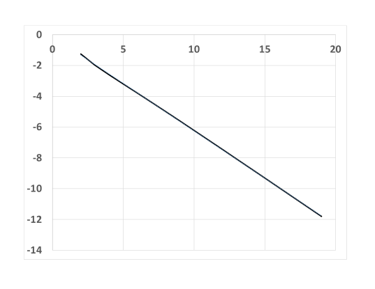
The results in this table suggest that as mm\to\infty

tc2τ2σ,γP,γQ1t_{c}\to 2\qquad\tau\to 2\qquad\sigma,\gamma_{P},\gamma_{Q}\to 1 (24)

It is clear from the table that β0\beta\to 0 but the question is: how fast? Figure 1 suggests that β0\beta\to 0 exponentially fast. If so then mβ0m\beta\to 0 and the conjectures about critical exponents in (24) follow

Refer to caption
Figure 1: Using data from Table I in [9] which gives estimates of β\beta for m=2m=2 to 20 and plotting log10β\log_{10}\beta versus mm we get a straight line log10β=0.615m0.0915\log_{10}\beta=-0.615m-0.0915. For the fit r2=0.9999r^{2}=0.9999.

Example 2. Median(2m-1) rule. It would be interesting to know if this models and Min(m) have the same value of β\beta and hence all the critical exponents are the same. This conjecture is based on the notion of a universality class of models. For example if one considers bond or site percolation on different two-dimensional lattices (rectangular, triangular, hexagonal, etc) then the critical values for the existence of an infinite component are different but the critical exponents are expected to be the same. Likewise the dd-dimensional contact process ie expected to have exponents that are do not depend on the neighborhood used to define the model and will have the same cirtical exponents as oriented percolation in (d+1)(d+1) dimensions.

Theorem 1 implies that the Min(m) models are in different universlaity classes (if the values of Δ\Delta are the same for \ell and mm then (21)β=(2m1)βm(2\ell-1)\beta_{\ell}=(2m-1)\beta_{m} the values of τ2\tau-2 must be different). Sabbir and Hassam [25] claim that the sum and the product rule defined in the next section have the same critical exponents, but otherwise it seems that within this class of models, the universality classes are small.

The next result treats our other two models.

Theorem 2.

In the case of the Max(m) and BF vertex rules we have

γϕ=γ=1\displaystyle\gamma_{\phi}=\gamma=1
Δ=1/σ=1+β\displaystyle\Delta=1/\sigma=1+\beta
τ2=β1+β\displaystyle\tau-2=\frac{\beta}{1+\beta}

Again if we know β\beta we can calculate all of the exponents, but this time we want to do more. As explained in the next section, the BF vertex rule is a bounded size rule, so it follows from work of Riordan and Warnke [24] that all the critical exponents are the same Erdös-Rényi We think it might be possible to use the proof of Theorem 6 to prove τ=5/2\tau=5/2 for the Max(m) rule or any other system in which ϕcp\phi\sim cp.

While in principle we can study two-edge rules in which the choice functions are different, in practice we can only analyze the case in which the first choice is a randomly chosen vertex,

Example 5. Adjacent edge rule. D’Souza and MItzenmacher [11] considered the case where the first vertex is chosen at random and the second according the min rule. They restricted their attention to the case m=2m=2 but here we consider the general situation.

Generalizing the proofs of Lemmas 4 and 6 in Section 4.2

θ(t)/t\displaystyle\partial\theta(t)/\partial t =spΦ+sϕθ\displaystyle=\langle s\rangle_{p}\Phi+\langle s\rangle_{\phi}\theta
sP/t\displaystyle\partial\langle s\rangle_{P}/\partial t =2sϕsps2pΦs2ϕθ\displaystyle=2\langle s\rangle_{\phi}\langle s\rangle_{p}-\langle s^{2}\rangle_{p}\Phi-\langle s^{2}\rangle_{\phi}\theta

From this it follows that

β1\displaystyle\beta-1 =min{βγϕ,βϕγ}\displaystyle=\min\{\beta-\gamma_{\phi},\beta_{\phi}-\gamma\} (25)
γ1\displaystyle-\gamma-1 =γϕγ\displaystyle=\gamma_{\phi}-\gamma (26)

where in the second equation we have only used the limit ttct\uparrow t_{c}. Generalizing the proof of (23) we can conclude that

σ=α+2\sigma=\alpha+2 (27)

Combining our results we have

Theorem 3.

In the case of the alternative edge rules we have

γϕ=1\displaystyle\gamma_{\phi}=1
γ=1+(m1)β\displaystyle\gamma=1+(m-1)\beta
Δ=1/σ=1+mβ\displaystyle\Delta=1/\sigma=1+m\beta
τ2=β1+mβ\displaystyle\tau-2=\frac{\beta}{1+m\beta}

At the moment we are only able to prove the second result under the assumption that βγϕ=βϕγ\beta-\gamma_{\phi}=\beta_{\phi}-\gamma. In support of this belief we refer the reader to the sketch of the proof of (23).

2 Achlioptas processes

In this section we review previous work.

2.1 Bounded size rules

Bohman and Frieze [6] were the first to describe a rule that made percolation come later than in the Erdös-Rényi case. Again G0=0G_{0}=0 and edges e1,e1;e2,e2;e3,e3e_{1},e_{1}^{\prime};e_{2},e_{2}^{\prime};e_{3},e_{3}^{\prime}\ldots are chosen at random from the set of all possible edges. If on the iith step eie_{i} connects two isolated vertices it is added to the graph, otherwise eie_{i}^{\prime} is added. Using our convention that the graph after kk choices is the sate at time to time 2k/n,2k/n, then as nn\to\infty They showed that

Theorem 4.

There is a constant c0>1.07c_{0}>1.07 so that the largest component at time c0c_{0} has size bounded by (logn)O(1)(\log n)^{O(1)}

This is an example of a bounded size rule. In these systems the decisions about which edge to add is based on the sizes of the components of the vertices chosen, with all of the components of size κiK\kappa_{i}\geq K being treated the same. Spencer and Wormald [26] developed a number of important results for the bounded-size case. To state their “main result let

S(G)=1nv|𝒞(v)|=1n|𝒞i2|S(G)=\frac{1}{n}\sum_{v}|{\cal C}(v)|=\frac{1}{n}|{\cal C}_{i}^{2}|

be the susceptibility, which in percolation terminology is just the mean cluster size. They showed, among other things, that

Theorem 5.

The critical value tct_{c} for the emergence of a giant cmponents can be defined by limttcS(t)=\lim_{t\uparrow t_{c}}S(t)=\infty.

As in ordinary percxolation, when t>tct>t_{c} there is a giant component containing a positive fraction of the sites, while for t<tct<t_{c} the cluster size distribution has P(κs)KecsP(\kappa\geq s)\leq Ke^{-cs} where KK and cc depend on tt.

In 2013, Bhamidi, Budhirja and Wang [5] showed that the behavior of the Bohman-Frieze process near the critical values is the same as in the Erdös-Rényi case. To be precise if we consider the behavior at tc+r/n1/3t_{c}+r/n^{1/3} with <r<-\infty<r<\infty then as nn\to\infty the system converges to the multiplicative coalecsent in which a cluster of size xx and a cluster of size yy merge at rate xyxy. See Aldous [2] for the corresponding result for Erdös-Rényi graphs.

Theorem 6.

There are constants α,β>0\alpha,\beta>0 the Bohman-Frieze process at time and let 𝒞in{\cal C}^{n}_{i} be the clusters writtein in order of decreasing size then then the vector of component sizes

β1/3n2/3|𝒞in|(tc+αβ2/3r/n1/3)\frac{\beta^{1/3}}{n^{2/3}}|{\cal C}^{n}_{i}|(t_{c}+\alpha\beta^{2/3}r/n^{1/3})\qquad

viewed as a function of r(,)r\in(-\infty,\infty) converges to multiplicative coalescent.

Riordan and Warnke [24] have show that “bounded-size rules share (in a strong sense) all the features of the Erdös-Rényi phase transiiton.” Let LjL_{j} be the size of the jjth largest component and let

Sr=𝒞|𝒞|/n=k1kr1Nk/nS_{r}=\sum_{{\cal C}}|{\cal C}|/n=\sum_{k\geq 1}k^{r-1}N_{k}/n

where the first sum is over all components and NkN_{k} is the number of vertices that belong to components of size kk. Writing whp (with high probability) for with probaility tending to 1 as nn\to\infty they established (see their Theorem 1.1):

Theorem 7.

Let {\cal R} be a bounded-size rule with critical time tc>0t_{c}>0. There are rule dependent positive constants a,A,c,C,γa,A,c,C,\gamma and BrB_{r}, r2r\geq 2 so that for any ϵ0\epsilon\to 0 with ϵ3n\epsilon^{3}n\to\infty as nn\to\infty

1. (Subcritical phase) For any fixed j1j\geq 1 and r2r\geq 2

Lj(tcnϵn)Cϵ2log(ϵ3n)\displaystyle L_{j}(t_{c}n-\epsilon n)\sim C\epsilon^{-2}\log(\epsilon^{3}n)
Sr(tcnϵn)Brϵ2r+3\displaystyle S_{r}(t_{c}n-\epsilon n)\sim B_{r}\epsilon^{-2r+3}

2. (Subcritical phase) For any fixed j1j\geq 1 and r2r\geq 2

L1(tcn+ϵn)cϵn\displaystyle L_{1}(t_{c}n+\epsilon n)\sim c\epsilon n
L2(tcn+ϵn)=o(ϵn)\displaystyle L_{2}(t_{c}n+\epsilon n)=o(\epsilon n)

3. (Critical regime) Suppose that k=k(n)1k=k(n)\geq 1 and ϵ=ϵ(n)>0\epsilon=\epsilon(n)>0 satisfy knγk\leq n^{\gamma}, ϵ2nγlogn\epsilon^{2}n\leq\gamma\log n, kk\to\infty, and ϵ3k0\epsilon^{3}k\to 0

Nk(tc±ϵn)Ak3/2eaϵ2knN_{k}(t_{c}\pm\epsilon n)\sim Ak^{-3/2}e^{-a\epsilon^{2}k}n

2.2 Explosive percolation

In 2009 Achliptas, D’Souza, and Spencer [1] shouted from the pages of Science that they had found “Explosive percolation in networks.” To quote from their paper:

Here we provide conclusive numerical evidence that unbounded size rules can give rise to discontinuous transitions. For concreteness, we present results for the so-called product rule.

To be precise, and changing notation to avoid conflict with ours, let L1(m)L_{1}(m) be the size of the largest cluster when there are mm edges, let m1m_{1} be the last time L1(m)<n1/2L_{1}(m)<n^{1/2}, and let m2m_{2} be the first time it is L(m)>n/2L(m)>n/2. Then for large nn we have m2m1<n2/3m_{2}-m_{1}<n^{2/3}.

In 2011 Riordan and Warnke wrote their own Science paper declaring that “Explosive percolation is continuous.” Here we will follow the version published the next year in the Annals of Applied Probability. [22]. The continuity of the phase transition is proved for a very general set of models

\ell-vertex rule. Let vm=(vm,1,vm,)v_{m}=(v_{m,1},\ldots v_{m,\ell}) be an i.i.d. sequence of vectors in {1,2,n}\{1,2,\ldots n\}^{\ell}. G0=G_{0}=\emptyset and GmG_{m} is obtained from Gm1G_{m-1} by adding a possibly empty set of edges EmE_{m}. EmE_{m}\neq\emptyset if the vi,mv_{i,m} are in distinct components.

Theorem 1 in [22]. Let {\cal R} be an \ell vertex rule with 2\ell\geq 2. Given any functions hL(n)h_{L}(n) and hm(n)h_{m}(n) that are o(n)o(n) and any constant δ>0\delta>0 the probability there are m1m_{1} and m2m_{2} with L1(m1)hL(n)L_{1}(m_{1})\leq h_{L}(n) and L1(m2)δnL_{1}(m_{2})\geq\delta n and m2m1+hM(n)m_{2}\leq m_{1}+h_{M}(n) tends to 0 as nn\to\infty.

To obtain more detailed results they reduced the collection of models. An \ell-vertex rule is said to be merging if whenever 𝒞1{\cal C}_{1} and 𝒞2{\cal C}_{2} are distinct components with |𝒞1|,|𝒞2|ϵn|{\cal C}_{1}|,|{\cal C}_{2}|\geq\epsilon n then in the next step we have probability ϵ\geq\epsilon^{\ell} of joining 𝒞1{\cal C}_{1} to 𝒞2{\cal C}_{2}.

Theorem 7 in [22]. Let {\cal R} be a merging \ell-vertex rule. Given constant 0a<b0\leq a<b and any function hm(n)=o(n)h_{m}(n)=o(n) the probability that there are m1m_{1} and m2m_{2} with L1(m1)anL_{1}(m_{1})\leq an and L1(m2)bnL_{1}(m_{2})\geq bn and m2m1+hm(n)m_{2}\leq m_{1}+h_{m}(n) tends to 0 as nn\to\infty.

This result gives a proof of Spencer’s “no two giants” conjecture. If at some time there is a component of size >ϵn>\epsilon n in addition to the giant component then when they merge the size will increase by at least ϵn\epsilon n contradicting the last result

The results in [22] are very general and their proofs are ingenious. However, the proof of their Theorem 1 given on page 1457 is based on an argument by contradiction, and it does not seem possible to extract quantitative result. Our goal here is to prove results about the critical behavior of some of these processes, specifically about the values of critical exponents defined in the next section.

3 Proofs of the Theorems

3.1 Proof of Theorem 1

Lemma 1 implies βϕ=mβ\beta_{\phi}=m\beta, ν=m\nu=m, so using (20)

β1=mβγϕorγϕ=1+(m1)β\beta-1=m\beta-\gamma_{\phi}\quad\hbox{or}\quad\gamma_{\phi}=1+(m-1)\beta

Using the first equality in (21) γ1=2γϕ-\gamma-1=-2\gamma_{\phi} so

γ=2γϕ+1=1+2(m1)β\gamma=2\gamma_{\phi}+1=1+2(m-1)\beta

To prove the next result we note that Lemma 1 implies

α=2m1mτ\alpha=2m-1-m\tau

and using (23) σ=(τ1)+2α+2\sigma=(\tau-1)+2\alpha+2

σ\displaystyle\sigma =τ1+2(2m1mτ)+2\displaystyle=\tau-1+2(2m-1-m\tau)+2
=1+2(2m1)(2m1)τ=1(2m1)(τ2)\displaystyle=1+2(2m-1)-(2m-1)\tau=1-(2m-1)(\tau-2) (28)

Dividing each side by σ\sigma and using (13) (τ2)/σ=β(\tau-2)/\sigma=\beta gives

1/σ=1+(2m1)β1/\sigma=1+(2m-1)\beta

Rearranging (28) then using the last result twice

τ2=1σ2m1=(1/σ1)/(2m1)1/σ=β1+(2m1)β\tau-2=\frac{1-\sigma}{2m-1}=\frac{(1/\sigma-1)/(2m-1)}{1/\sigma}=\frac{\beta}{1+(2m-1)\beta}

which completes the proof.

3.2 Proof of Theorem 2

Since ϕ\phi is Min(m), Lemma 1 implies βϕ=mβ\beta_{\phi}=m\beta so (20) implies γϕ=1\gamma_{\phi}=1 and (21) implies γ=1\gamma=1. Using (13), (14) and (15) we have

Δ=1/σ=β+γ=1+β\Delta=1/\sigma=\beta+\gamma=1+\beta

Using (13)

τ2=β1/σ=β1+β\tau-2=\frac{\beta}{1/\sigma}=\frac{\beta}{1+\beta}

which completes the proof.

3.3 Proof of Theorem 3

Lemma 1 implies βϕ=β\beta_{\phi}=\beta. (26) implies γϕ=1\gamma_{\phi}=1. The ϕ\phi versions of (13), (14) and (15) imply

Δ=1/σ=βϕ+γϕ=1+mβ\Delta=1/\sigma=\beta_{\phi}+\gamma_{\phi}=1+m\beta

(27) and (28) imply

σ=α+2=2m+1mτ=1m(τ2)\sigma=\alpha+2=2m+1-m\tau=1-m(\tau-2)

Rearranging gives

τ2=1σm=(1/σ1)/m1/σ=β1+mβ\tau-2=\frac{1-\sigma}{m}=\frac{(1/\sigma-1)/m}{1/\sigma}=\frac{\beta}{1+m\beta}

To get the final result we have to assume that the two quantities on the right hand side of (25) are equal, i.e. βγϕ=βϕγ\beta-\gamma_{\phi}=\beta_{\phi}-\gamma, in order to conclude that

γ=1+(m1)β\gamma=1+(m-1)\beta

4 Proofs of scaling relations

4.1 Results that follow from (1)

To have rigorous result we state explicitly what we assume about τ\tau and about the scaling function. Throughout we only use the scaling relationship

p(s,t)=s1τf(s|ttc|1/σ)p(s,t)=s^{1-\tau}f(s|t-t_{c}|^{1/\sigma})

Since ϕ(s,t)=s1τϕg(s|ttc|1/σ)\phi(s,t)=s^{1-\tau_{\phi}}g(s|t-t_{c}|^{1/\sigma}) the ϕ\phi versions of the scaling relationships follow immediately.

Lemma 2.

If 2<τ<32<\tau<3 and ff is bounded, and is Lipschitz continuous at 0.

β=(τ2)/σ\beta=(\tau-2)/\sigma
Proof.

Using (1) and replacing sum by integration.

θ(t)1s1τ[f(0)f(sδ1/σ)]𝑑s\theta(t)\approx\int_{1}^{\infty}s^{1-\tau}[f(0)-f(s\delta^{1/\sigma})]\,ds

Changing variables s=xδ1/σs=x\delta^{-1/\sigma}, ds=δ1/σdxds=\delta^{-1/\sigma}dx the above

=δ(τ2)/σδ1/σx1τ[f(0)f(x)]𝑑x=\delta^{(\tau-2)/\sigma}\int_{\delta^{1/\sigma}}^{\infty}x^{1-\tau}[f(0)-f(x)]\,dx

Since ff is bounded and τ>2\tau>2 the integral over [1,)[1,\infty) is finite. Since ff is Lipschitz continuous the integrand is Cx2τ\leq Cx^{2-\tau} near 0. Since γ<3\gamma<3, the integral over [0,1][0,1] is finite, and it follows that θ(t)Cδ(τ2)/σ\theta(t)\sim C\delta^{(\tau-2)/\sigma}. ∎

The next result establishes (14) and (15)

Lemma 3.

If 2<γ<32<\gamma<3 and 1xmf(x)𝑑x<\int_{1}^{\infty}x^{m}f(x)\,dx<\infty for all mm then for all ρ1\rho\geq 1

Γ(r)=(r+2τ)/σ\Gamma(r)=(r+2-\tau)/\sigma

It follows that for all integers k2k\geq 2,

Δk=Γ(k)Γ(k1)=1/σ.\Delta_{k}=\Gamma(k)-\Gamma(k-1)=1/\sigma.
Proof.
E|𝒞x|r=1sr+1τf(sδ1/σ)𝑑sE|{\cal C}_{x}|^{r}=\int_{1}^{\infty}s^{r+1-\tau}f(s\delta^{1/\sigma})\,ds (29)

Changing variables s=xδ1/σs=x\delta^{-1/\sigma}, ds=δ1/σdxds=\delta^{-1/\sigma}dx the above

=δ(τ2r)/σδ1/σxρ+1τf(x)𝑑x=\delta^{(\tau-2-r)/\sigma}\int_{\delta^{1/\sigma}}^{\infty}x^{\rho+1-\tau}f(x)\,dx

The assumption 1xmf(x)𝑑x<\int_{1}^{\infty}x^{m}f(x)\,dx<\infty for all mm implies that the integral over [1,)[1,\infty) is finite. Since τ<3\tau<3 and ρ1\rho\geq 1 the integral over [0,1][0,1] is finite ∎

4.2 Proofs of ODE consequences

We will now derive two consequences of the ODE for two-choice rules (LABEL:genODE). Let θ(t)=1i=1p(1,t)\theta(t)=1-\sum_{i=1}^{\infty}p(1,t) be the fraction of vertices in giant components. The first result establishes (20)

Lemma 4.

Let Φ=1vϕ(v,t)\Phi=1-\sum_{v}\phi(v,t) and sϕ=ssϕ(s,t)\langle s\rangle_{\phi}=\sum_{s}s\phi(s,t)

θ(t)t=2sϕΦ\frac{\partial\theta(t)}{\partial t}=2\langle s\rangle_{\phi}\Phi
Proof.

θ(t)=1sP(s,t)\theta(t)=1-\sum_{s}P(s,t) so we have

θt\displaystyle\frac{\partial\theta}{\partial t} =sPt=ssu+v=sϕ(u,t)ϕ(v,t)+s2sϕ(s,t)\displaystyle=-\sum_{s}\frac{\partial P}{\partial t}\ =-\sum_{s}s\sum_{u+v=s}\phi(u,t)\phi(v,t)+\sum_{s}2s\phi(s,t)
=uv(u+v)ϕ(u,t)ϕ(v,t)+s2sϕ(s,t)\displaystyle=-\sum_{u}\sum_{v}(u+v)\phi(u,t)\phi(v,t)+\sum_{s}2s\phi(s,t)
=2uuϕ(u,t)vϕ(v,t)+s2sϕ(s,t)\displaystyle=-2\sum_{u}u\phi(u,t)\sum_{v}\phi(v,t)+\sum_{s}2s\phi(s,t)
=2ssϕ(s,t)[1vϕ(v,t)]=2sϕΦ\displaystyle=2\sum_{s}s\phi(s,t)\left[1-\sum_{v}\phi(v,t)\right]=2\langle s\rangle_{\phi}\Phi

which proves the desired result. ∎

While the proof is fresh on the readers mind we will prove the result for the alternate edge rule.

Lemma 5.
θ(t)t=spϕ+sϕθ\frac{\partial\theta(t)}{\partial t}=\langle s\rangle_{p}\phi+\langle s\rangle_{\phi}\theta
Proof.

Computing as above using the alterantive edge ODE

θt\displaystyle\frac{\partial\theta}{\partial t} =uv(u+v)p(u,t)ϕ(v,t)+ssp(s,t)+ssϕ(s,t)\displaystyle=-\sum_{u}\sum_{v}(u+v)p(u,t)\phi(v,t)+\sum_{s}sp(s,t)+\sum_{s}s\phi(s,t)
=uup(u,t)vϕ(v,t)+uup(u,t)\displaystyle=-\sum_{u}up(u,t)\sum_{v}\phi(v,t)+\sum_{u}up(u,t)
vvϕ(v,t)uϕ(u,t)+vvψ(u,t)\displaystyle-\sum_{v}v\phi(v,t)\sum_{u}\phi(u,t)+\sum_{v}v\psi(u,t)

which proves the desired result. ∎

We now prove the second result

Lemma 6.

sp/t=2sϕ22Φs2ϕ\partial\langle s\rangle_{p}/\partial t=2\langle s\rangle^{2}_{\phi}-2\Phi\langle s^{2}\rangle_{\phi}

Proof.

Multiplying by ss and then summing

spt\displaystyle\frac{\partial\langle s\rangle_{p}}{\partial t} =ss2u+v=sϕ(u,t)ϕ(v,t)s2s2ϕ(s,t)\displaystyle=\sum_{s}s^{2}\sum_{u+v=s}\phi(u,t)\phi(v,t)-\sum_{s}2s^{2}\phi(s,t)
=uv(u+v)2ϕ(u,t)ϕ(v,t)s2s2ϕ(s,t)\displaystyle=\sum_{u}\sum_{v}(u+v)^{2}\phi(u,t)\phi(v,t)-\sum_{s}2s^{2}\phi(s,t)
=2uuϕ(u,t)vvϕ(v,t)+2uu2ϕ(u,t)vϕ(v,t)s2s2ϕ(s,t)\displaystyle=2\sum_{u}u\phi(u,t)\sum_{v}v\phi(v,t)+2\sum_{u}u^{2}\phi(u,t)\sum_{v}\phi(v,t)-\sum_{s}2s^{2}\phi(s,t)
=2sϕ22Φs2ϕ\displaystyle=2\langle s\rangle^{2}_{\phi}-2\Phi\langle s^{2}\rangle_{\phi}

which gives the desired result. ∎

Again our next step is to extend to the alternative edge rule.

Lemma 7.

sp/t=2spsϕΦs2pθs2ϕ\partial\langle s\rangle_{p}/\partial t=2\langle s\rangle_{p}\langle s\rangle_{\phi}-\Phi\langle s^{2}\rangle_{p}-\theta\langle s^{2}\rangle_{\phi}

Proof.

Multiplying by ss and then summing

spt\displaystyle\frac{\partial\langle s\rangle_{p}}{\partial t} =uv(u+v)2p(u,t)ϕ(v,t)ss2p(s,t)ss2ϕ(s,t)\displaystyle=\sum_{u}\sum_{v}(u+v)^{2}p(u,t)\phi(v,t)-\sum_{s}s^{2}p(s,t)-\sum_{s}s^{2}\phi(s,t)
=2uup(u,t)vvϕ(v,t)\displaystyle=2\sum_{u}up(u,t)\sum_{v}v\phi(v,t)
+uu2p(u,t)vϕ(v,t)ss2p(s,t)\displaystyle+\sum_{u}u^{2}p(u,t)\sum_{v}\phi(v,t)-\sum_{s}s^{2}p(s,t)
+vv2ϕ(v,t)up(v,t)ss2ϕ(s,t)\displaystyle+\sum_{v}v^{2}\phi(v,t)\sum_{u}p(v,t)-\sum_{s}s^{2}\phi(s,t)

which gives the desired result. ∎

4.3 A computation from Appendix E of [10]

Their argument is for the 2 choice min rule. To generalize we suppose

ϕ(s,t)=sαg(sδ1/σ)\phi(s,t)=s^{\alpha}g(s\delta^{1/\sigma})

It is convenient to let f(x)=xτ1f~(x)f(x)=x^{\tau-1}\tilde{f}(x), and g(x)=xαg~(x)g(x)=x^{-\alpha}\tilde{g}(x) in order to rewrite the scaling formulas as

p(s,t)\displaystyle p(s,t) =s1τf(sδ1/σ)=δ(τ1)/σf~(sδ1/σ)\displaystyle=s^{1-\tau}f(s\delta^{1/\sigma})=\delta^{(\tau-1)/\sigma}\tilde{f}(s\delta^{1/\sigma}) (30)
ϕ(s,t)\displaystyle\phi(s,t) =sαg(sδ1/σ)=δα/σg~(sδ1/σ)\displaystyle=s^{\alpha}g(s\delta^{1/\sigma})=\delta^{-\alpha/\sigma}\tilde{g}(s\delta^{1/\sigma}) (31)

To eliminate the contribution from small values of uu and vv we substitute ϕ(u)=ϕ(u)ϕ(s)+ϕ(s)\phi(u)=\phi(u)-\phi(s)+\phi(s) and ϕ(su)=ϕ(su)ϕ(s)+ϕ(s)\phi(s-u)=\phi(s-u)-\phi(s)+\phi(s) in (LABEL:genODE) to get

p(s)t=su=1s1ϕ(u)ϕ(su)2sϕ(s)\displaystyle\frac{\partial p(s)}{\partial t}=s\sum_{u=1}^{s-1}\phi(u)\phi(s-u)-2s\phi(s)
=su=1s1[ϕ(u)ϕ(s)][ϕ(su)ϕ(s)]\displaystyle=s\sum_{u=1}^{s-1}[\phi(u)-\phi(s)][\phi(s-u)-\phi(s)]
+su=1s1ϕ(s)ϕ(su)+su=1s1ϕ(u)ϕ(s)su=1s1ϕ(s)22sϕ(s)\displaystyle+s\sum_{u=1}^{s-1}\phi(s)\phi(s-u)+s\sum_{u=1}^{s-1}\phi(u)\phi(s)-s\sum_{u=1}^{s-1}\phi(s)^{2}-2s\phi(s)

where we have dropped the dependence on tt to simplify the formulas.

Rearranging gives

p(s)t\displaystyle\frac{\partial p(s)}{\partial t} =su=1s1[ϕ(u)ϕ(s)][ϕ(su)ϕ(s)]\displaystyle=s\sum_{u=1}^{s-1}[\phi(u)-\phi(s)][\phi(s-u)-\phi(s)]
+2sϕ(s)[1u=sϕ(u)]s(s1)ϕ(s)22sϕ(s)\displaystyle+2s\phi(s)\left[1-\sum_{u=s}^{\infty}\phi(u)\right]-s(s-1)\phi(s)^{2}-2s\phi(s)

Canceling the two 2sϕ(s)2s\phi(s) and writing in integral form

p(s)t\displaystyle\frac{\partial p(s)}{\partial t} =s2ϕ2(s)2sϕ(s)sϕ(u)𝑑u\displaystyle=-s^{2}\phi^{2}(s)-2s\phi(s)\int_{s}^{\infty}\phi(u)\,du
+s0s[ϕ(u)ϕ(s)][ϕ(su)ϕ(s)]𝑑u\displaystyle+s\int_{0}^{s}[\phi(u)-\phi(s)][\phi(s-u)-\phi(s)]\,du (32)

Taking δ=tct\delta=t_{c}-t and using sδ1/σ=xs\delta^{-1/\sigma}=x with p(s,t)=δ(τ1)/σf~(sδ1/σ)p(s,t)=\delta^{(\tau-1)/\sigma}\tilde{f}(s\delta^{1/\sigma})

pt\displaystyle\frac{\partial p}{\partial t} =τ1σδ1+(τ1)/σf~(sδ1/σ)δ(τ1)/σf~(sδ1/σ)sσδ1+1/σ\displaystyle=-\frac{\tau-1}{\sigma}\delta^{-1+(\tau-1)/\sigma}\tilde{f}(s\delta^{1/\sigma})-\delta^{(\tau-1)/\sigma}\tilde{f}^{\prime}(s\delta^{1/\sigma})\frac{s}{\sigma}\delta^{-1+1/\sigma}
=[τ1σf~(x)xσf~(x)]δ1+(τ1)/σ\displaystyle=\left[-\frac{\tau-1}{\sigma}\tilde{f}(x)-\frac{x}{\sigma}\tilde{f}^{\prime}(x)\right]\cdot\delta^{-1+(\tau-1)/\sigma} (33)

Using ϕ(r)=δα/σg~(rδ1/σ)\phi(r)=\delta^{-\alpha/\sigma}\tilde{g}(r\delta^{1/\sigma}) the right-hand side of (32) becomes

=s2δ2α/σg~(sδ1/σ)22sδ2α/σg~(sδ1/σ)s𝑑ug~(uδ1/σ)\displaystyle=-s^{2}\delta^{-2\alpha/\sigma}\tilde{g}(s\delta^{1/\sigma})^{2}-2s\delta^{-2\alpha/\sigma}\tilde{g}(s\delta^{1/\sigma})\int_{s}^{\infty}du\,\tilde{g}(u\delta^{1/\sigma})
+sδ2α/σ0s𝑑u[g~(uδ1/σ)g~(sδ1/σ)][g~((su)δ1/σ)g~(sδ1/σ)]\displaystyle+s\delta^{-2\alpha/\sigma}\int_{0}^{s}du\,[\tilde{g}(u\delta^{1/\sigma})-\tilde{g}(s\delta^{1/\sigma})]\cdot[\tilde{g}((s-u)\delta^{1/\sigma})-\tilde{g}(s\delta^{1/\sigma})]

using s=xδ1/σs=x\delta^{-1/\sigma}, u=yδ1/σu=y\delta^{-1/\sigma}, and du=dyδ1/σdu=dy\,\delta^{-1/\sigma}

=x2δ(2α2)/σg~(x)22xδ(2α2)/σx𝑑yg~(y)\displaystyle=-x^{2}\delta^{(-2\alpha-2)/\sigma}\tilde{g}(x)^{2}-2x\delta^{(-2\alpha-2)/\sigma}\int_{x}^{\infty}dy\,\tilde{g}(y)
+xδ(2α2)/σ0x𝑑y[g~(y)g~(x)],[g~(xy)g~(x)]\displaystyle+x\delta^{(-2\alpha-2)/\sigma}\int_{0}^{x}dy\,[\tilde{g}(y)-\tilde{g}(x)],[\tilde{g}(x-y)-\tilde{g}(x)] (34)

In order for (32) to hold the powers of δ\delta must be the same, i.e.

1+τ1σ=2α2σ-1+\frac{\tau-1}{\sigma}=\frac{-2\alpha-2}{\sigma}

Rearranging gives

σ=(τ1)+2α+2\sigma=(\tau-1)+2\alpha+2 (35)

4.4 Proof for adjacent edge rule

To eliminate the contribution from small values of uu and vv in (LABEL:genODE) we again substitute p(u)=p(u)p(s)+p(s)p(u)=p(u)-p(s)+p(s) and ϕ(su)=ϕ(su)ϕ(s)+ϕ(s)\phi(s-u)=\phi(s-u)-\phi(s)+\phi(s) to get

p(s)t=su=1s1p(u)ϕ(su)sp(s)sϕ(s)\displaystyle\frac{\partial p(s)}{\partial t}=s\sum_{u=1}^{s-1}p(u)\phi(s-u)-sp(s)-s\phi(s)
=su=1s1[p(u)p(s)][ϕ(su)ϕ(s)]\displaystyle=s\sum_{u=1}^{s-1}[p(u)-p(s)][\phi(s-u)-\phi(s)]
+su=1s1p(s)ϕ(su)+su=1s1p(u)ϕ(s)su=1s1p(s)ϕ(s)sp(s)sϕ(s)\displaystyle+s\sum_{u=1}^{s-1}p(s)\phi(s-u)+s\sum_{u=1}^{s-1}p(u)\phi(s)-s\sum_{u=1}^{s-1}p(s)\phi(s)-sp(s)-s\phi(s)

Rearranging gives

p(s)t\displaystyle\frac{\partial p(s)}{\partial t} =su=1s1[p(u)p(s)][ϕ(su)ϕ(s)]\displaystyle=s\sum_{u=1}^{s-1}[p(u)-p(s)][\phi(s-u)-\phi(s)]
+sp(s)v=1s1ϕ(v)+sϕ(s)u=1s1p(u)s(s1)p(s)ϕ(s)sp(s)sϕ(s)\displaystyle+sp(s)\sum_{v=1}^{s-1}\phi(v)+s\phi(s)\sum_{u=1}^{s-1}p(u)-s(s-1)p(s)\phi(s)-sp(s)-s\phi(s)

Canceling and writing in integral form

p(s)t=\displaystyle\frac{\partial p(s)}{\partial t}= s2p(s)ϕ(s)sp(s)sϕ(u)𝑑usϕ(s)sp(u)𝑑u\displaystyle-s^{2}p(s)\phi(s)-sp(s)\int_{s}^{\infty}\phi(u)\,du-s\phi(s)\int_{s}^{\infty}p(u)\,du
+s0s[p(u)p(s)][ϕ(su)ϕ(s)]𝑑u\displaystyle+s\int_{0}^{s}[p(u)-p(s)][\phi(s-u)-\phi(s)]\,du (36)

The formula for the left hand side given in (33) remains the same. Using p(r)=δ(τ1)/σf~(rδ1/σ)p(r)=\delta^{(\tau-1)/\sigma}\tilde{f}(r\delta^{1/\sigma}) ϕ(r)=δα/σg~(rδ1/σ)\phi(r)=\delta^{-\alpha/\sigma}\tilde{g}(r\delta^{1/\sigma}) the right-hand side is

=s2δ(τ1α)/σf~(sδ1/σ)g~(sδ1/σ)\displaystyle=-s^{2}\delta^{(\tau-1-\alpha)/\sigma}\tilde{f}(s\delta^{1/\sigma})\tilde{g}(s\delta^{1/\sigma})
sδ(τ1α)/σf~(sδ1/σ)s𝑑ug~(uδ1/σ)sδ(τ1α)/σg~(sδ1/σ)s𝑑uf~(uδ1/σ)\displaystyle-s\delta^{(\tau-1-\alpha)/\sigma}\tilde{f}(s\delta^{1/\sigma})\int_{s}^{\infty}du\,\tilde{g}(u\delta^{1/\sigma})-s\delta^{(\tau-1-\alpha)/\sigma}\tilde{g}(s\delta^{1/\sigma})\int_{s}^{\infty}du\,\tilde{f}(u\delta^{1/\sigma})
+sδ(τ1α)/σ0s𝑑u[f~(uδ1/σ)f~(sδ1/σ)][g~((su)δ1/σ)g~(sδ1/σ)]\displaystyle+s\delta^{(\tau-1-\alpha)/\sigma}\int_{0}^{s}du\,[\tilde{f}(u\delta^{1/\sigma})-\tilde{f}(s\delta^{1/\sigma})]\cdot[\tilde{g}((s-u)\delta^{1/\sigma})-\tilde{g}(s\delta^{1/\sigma})]

Using s=xδ1/σs=x\delta^{-1/\sigma}, u=yδ1/σu=y\delta^{-1/\sigma} du=dyδ1/σdu=dy\,\delta^{-1/\sigma}

=x2δ(τ1α2)/σf~(x)g~(x)\displaystyle=-x^{2}\delta^{(\tau-1-\alpha-2)/\sigma}\tilde{f}(x)\tilde{g}(x)
xδ(τ1α2)/σf~(x)x𝑑yg~(y)xδ(τ1α2)/σg~(x)s𝑑yf~(y)\displaystyle-x\delta^{(\tau-1-\alpha-2)/\sigma}\tilde{f}(x)\int_{x}^{\infty}dy\,\tilde{g}(y)-x\delta^{(\tau-1-\alpha-2)/\sigma}\tilde{g}(x)\int_{s}^{\infty}dy\,\tilde{f}(y)
+xδ(τ1α2)/σ0x𝑑y[f~(y)f~(x)][g~(xy)g~(x)]\displaystyle+x\delta^{(\tau-1-\alpha-2)/\sigma}\int_{0}^{x}dy\,[\tilde{f}(y)-\tilde{f}(x)]\cdot[\tilde{g}(x-y)-\tilde{g}(x)]

In order for (36) to hold the powers of δ\delta must be the same, i.e.

1+τ1σ=τ1α2σ-1+\frac{\tau-1}{\sigma}=\frac{\tau-1-\alpha-2}{\sigma}

Rearranging gives

σ=α+2\sigma=\alpha+2 (37)

5 Erdös-Rényi model

5.1 Survival probability

Let xx be a randomly chosen vertex and let ZmZ_{m} be the number of vertices at distance mm from xx. When m=o(logn)m=o(\log n) the cluster containing xx is whp a tree and ZmZ_{m} is a branching process in which each individual in generation mm has a Poisson(μ\mu) number of offespring.

Consider a branching process with offspring distribution rkr_{k} with mean μ>1\mu>1 and finite second moment. Let ϕ(z)=k=0rkzz\phi(z)=\sum_{k=0}^{\infty}r_{k}z^{z} be the generating function. If rKr_{K} is Poisson(μ\mu) then

ϕ(z)=k=0eμμk|k!zkexp(μ(1z))\phi(z)=\sum_{k=0}^{\infty}e^{-\mu}\frac{\mu^{k}|}{k!}z^{k}\exp(-\mu(1-z)) (38)

Let ρ\rho be probability the system dies out. Breaking things down according to the number of children in the first generation

ρ=k=0rkρk=ϕ(ρ)\rho=\sum_{k=0}^{\infty}r_{k}\rho^{k}=\phi(\rho)

ρ(1)=1\rho(1)=1 is a trivial solution. ρ\rho is the unique solution of ϕ(ρ)=ρ\phi(\rho)=\rho in [0,1)[0,1).

ϕ(1)=1ϕ(1)=k=0krk=μϕ′′(1)=k=0k(k1)rk=μ2\phi(1)=1\qquad\phi^{\prime}(1)=\sum_{k=0}^{\infty}kr_{k}=\mu\qquad\phi^{\prime\prime}(1)=\sum_{k=0}^{\infty}k(k-1)r_{k}=\mu_{2}

If μ\mu is close to 1 then ρ\rho will be close to 1. Ignoring a few details, if xx is close to 1 expanding ϕ\phi in power series around 1 gives

ϕ(1x)=1μx+μ2x2/2\phi(1-x)=1-\mu x+\mu_{2}x^{2}/2

so for a fixed point we want

(μ1)x=μ2x2/2(\mu-1)x=\mu_{2}x^{2}/2

or x=2(μ1)/μ2x=2(\mu-1)/\mu_{2}. If we let θ(μ)=P(|𝒞x|=)\theta(\mu)=P(|{\cal C}_{x}|=\infty) which is the same as the fraction of vertices in the giant component

θ(μ)2μ2(μ1)\theta(\mu)\sim\frac{2}{\mu_{2}}(\mu-1) (39)

so the critical exponent β=1\beta=1.

5.2 Mean cluster size.

Let 𝒞x{\cal C}_{x} be the cluster containing xx. If μ<1\mu<1

E|𝒞x|=1+μ+μ2+=11μ.E|{\cal C}_{x}|=1+\mu+\mu^{2}+\cdots=\frac{1}{1-\mu}. (40)

so γ=1\gamma=1. In the supercritical regime we consider

E(|𝒞x|;|𝒞x|<)E(|{\cal C}_{x}|;|{\cal C}_{x}|<\infty)

The cluster size is the same as the total progeny in a supercritical branching process conditioned to die out.

Theorem 8.

A supercritical branching process conditioned to become extinct is a subcritical branching process. If the original offspring distribution is Poisson(μ\mu) with μ>1\mu>1 then the conditioned one is Poisson(μρ\mu\rho) where ρ\rho is the extinction probability.

Proof.

Let T0=inf{t:Zt=0}T_{0}=\inf\{t:Z_{t}=0\} and consider Z¯t=(Zt|T0<)\bar{Z}_{t}=(Z_{t}|T_{0}<\infty). To check the Markov property for Z¯t\bar{Z}_{t} note that the Markov property for ZtZ_{t} implies:

P(Zt+1=zt+1,T0<|Zt=zt,Z0=z0)=P(Zt+1=zt+1,T0<|Zt=zt)P(Z_{t+1}=z_{t+1},T_{0}<\infty|Z_{t}=z_{t},\ldots Z_{0}=z_{0})=P(Z_{t+1}=z_{t+1},T_{0}<\infty|Z_{t}=z_{t})

To compute the transition probability for Z¯t\bar{Z}_{t}, observe that if ρ\rho is the extinction probability then Px(T0<)=ρxP_{x}(T_{0}<\infty)=\rho^{x}. Let p(x,y)p(x,y) be the transition probability for ZtZ_{t}. Note that the Markov property implies

p¯(x,y)=Px(Z1=y,T0<)Px(T0<)=Px(Z1=y)Py(T0<)Px(T0<)=p(x,y)ρyρx\bar{p}(x,y)=\frac{P_{x}(Z_{1}=y,T_{0}<\infty)}{P_{x}(T_{0}<\infty)}=\frac{P_{x}(Z_{1}=y)P_{y}(T_{0}<\infty)}{P_{x}(T_{0}<\infty)}=\frac{p(x,y)\rho^{y}}{\rho^{x}}

Taking x=1x=1 and computing the generating function

y=0p¯(1,y)zy=ρ1y=0p(1,y)(zρ)y=ρ1ϕ(zρ)\sum_{y=0}^{\infty}\bar{p}(1,y)z^{y}=\rho^{-1}\sum_{y=0}^{\infty}p(1,y)(z\rho)^{y}=\rho^{-1}\phi(z\rho) (41)

where py=p(1,y)p_{y}=p(1,y) is the offspring distribution.

p¯y=p¯(1,y)\bar{p}_{y}=\bar{p}(1,y) is the distribution of the size of the family of an individual, conditioned on the branching process dying out. If we start with xx individuals then in ZnZ_{n} each gives rise to an independent family. In Z¯n\bar{Z}_{n} each family must die out, so Z¯n\bar{Z}_{n} is a branching process with offspring distribution p¯(1,y)\bar{p}(1,y). To prove this formally observe that

p(x,y)=j1,jx0,j1++jx=ypj1pjxp(x,y)=\sum_{j_{1},\ldots j_{x}\geq 0,j_{1}+\cdots+j_{x}=y}p_{j_{1}}\cdots p_{j_{x}}

Writing \sum_{*} as shorthand for the sum in the last display

p(x,y)ρyρx=pj1ρj1ρpjxρjxρ=p¯j1p¯jx\frac{p(x,y)\rho^{y}}{\rho^{x}}=\sum_{*}\frac{p_{j_{1}}\rho^{j_{1}}}{\rho}\cdots\frac{p_{j_{x}}\rho^{j_{x}}}{\rho}=\sum_{*}\bar{p}_{j_{1}}\cdots\bar{p}_{j_{x}}

In the case of the Poisson(μ\mu) distribution ϕ(z)=exp(μ(z1))\phi(z)=\exp(\mu(z-1)) so if λ>1\lambda>1, so using (41)

ϕ(zρ)ρ=exp(μ(zρ1))exp(μ(ρ1))=exp(μρ(z1))\frac{\phi(z\rho)}{\rho}=\frac{\exp(\mu(z\rho-1))}{\exp(\mu(\rho-1))}=\exp(\mu\rho(z-1))

which completes the proof that the conditioned process is a Poisson(μρ\mu\rho) branching process ∎

Using the result for the subcritical case in (40)

E(|𝒞x|||𝒞x|<)=11μρE(|{\cal C}_{x}|\,|\,|{\cal C}_{x}|<\infty)=\frac{1}{1-\mu\rho}

Since μ2=μ2\mu_{2}=\mu^{2} for Poisson, (39) shows that if μ\mu is close to 1

ρ12(μ1)μ2\rho\approx 1-\frac{2(\mu-1)}{\mu^{2}}

so we have

1μρ=1μ+2(μ1)μ=2(μ1)μ(μ1)μ1-\mu\rho=1-\mu+\frac{2(\mu-1)}{\mu}=\frac{2(\mu-1)-\mu(\mu-1)}{\mu}

From this we see that

E(|𝒞x|||𝒞x|<)=11μρ1(1μ)E(|{\cal C}_{x}|\,|\,|{\cal C}_{x}|<\infty)=\frac{1}{1-\mu\rho}\sim\frac{1}{(1-\mu)}

thus the asymptotic behavior of the mean cluster size as μ1\mu\downarrow 1 is exactly the same as as μ1\mu\uparrow 1

5.3 Higher moments

Although the connection with clusters in Erdös-Rényi random graps and branching processes is intuitive, it is more convenient technically to expose the cluster one site at a time to obtain something that can be approximated by a random walk. Let ηx,y=ηy,x=1\eta_{x,y}=\eta_{y,x}=1 if there is an edge between xx and yy. Let RtR_{t} be the set of removed sites, UtU_{t} be the unexplored sites and AtA_{t} is the set of active sites. Initially R0=R_{0}=\emptyset, U0={2,3,,n}U_{0}=\{2,3,\ldots,n\}, and A0={1}A_{0}=\{1\}. If AtA_{t}\neq\emptyset, pick iti_{t} at random from AtA_{t} let

Rt+1\displaystyle R_{t+1} =Rt{it}\displaystyle=R_{t}\cup\{i_{t}\} (42)
At+1\displaystyle A_{t+1} =At{it}{yUt:ηit,y=1}\displaystyle=A_{t}-\{i_{t}\}\cup\{y\in U_{t}:\eta_{i_{t},y}=1\} (43)
Ut+1\displaystyle U_{t+1} =Ut{yUt:ηit,y=1}\displaystyle=U_{t}-\{y\in U_{t}:\eta_{i_{t},y}=1\} (44)

At time τ=inf{t:At=}\tau=\inf\{t:A_{t}=\emptyset\} we have found all the sites in the cluster and the process stops. |Rt|=t|R_{t}|=t for all tτt\leq\tau, so the cluster size is τ\tau. If |An|>0|A_{n}|>0 and the number of rermoved sites is small

Sn+1Sn1+Poisson(μ)S_{n+1}\approx S_{n}-1+\hbox{Poisson}(\mu)

To have the process defined for all time let ξ1,ξ2,\xi_{1},\xi_{2},\ldots be i.i.d. 1+Poisson(μ)-1+\hbox{Poisson}(\mu) and Sn+1=Sn+ξn+1S_{n+1}=S_{n}+\xi_{n+1}.

We begin by computing the moment generating function of ξi\xi_{i}

ψ(θ)=eθm=0eμμmm!=exp(θ+μ(eθ1))\psi(\theta)=e^{-\theta}\sum_{m=0}^{\infty}e^{-\mu}\frac{\mu^{m}}{m!}=\exp(-\theta+\mu(e^{\theta}-1)) (45)

exp(θSt)/ϕ(θ)t\exp(\theta S_{t})/\phi(\theta)^{t} is a nonnegative martingale, so using the optional stopping theorem for the nonnegative supermartingale Mt=exp(θSt)/ψ(θ)tM_{t}=\exp(\theta S_{t})/\psi(\theta)^{t}, see e.g., (7.6) in Chapter 4 of Durrett (2004)

M0=eθE(ψ(θ)τ)M_{0}=e^{\theta}\geq E(\psi(\theta)^{-\tau}) (46)

ψ(0)=Eξi=1μ\psi^{\prime}(0)=E\xi_{i}=1-\mu so if μ<1\mu<1 then ψ(θ)<1\psi(\theta)<1 when θ>0\theta>0 is small. To optimize we note that the derivative

ddθ(θ+μ(eθ1))=1+μeθ=0\frac{d}{d\theta}(-\theta+\mu(e^{\theta}-1))=-1+\mu e^{\theta}=0

when θ1=logμ\theta_{1}=-\log\mu. At this point eθ1=1/μe^{\theta_{1}}=1/\mu and

ψ(θ1)=exp(log(λ)+1λ)eα<1\psi(\theta_{1})=\exp(\log(\lambda)+1-\lambda)\equiv e^{-\alpha}<1

Since ψ(θ11=eα>1\psi(\theta_{1}^{-1}=e^{\alpha}>1, using Chebyshev’s inequality with (46)

eαmP(τm)=ψ(θ1)mP(τm)E(ψ(θ1)τ)eθ1e^{\alpha m}P(\tau\geq m)=\psi(\theta_{1})^{-m}P(\tau\geq m)\leq E(\psi(\theta_{1})^{-\tau})\leq e^{\theta_{1}}

One particle dies on each time step so 1+ξ1++ξτ=τ1+\xi_{1}+\cdots+\xi_{\tau}=\tau and we have

P(max0nτSnm)emα/μP\left(\max_{0\leq n\leq\tau}S_{n}\geq m\right)\leq e^{-m\alpha}/\mu (47)

There are several other martingale associated with a random walk. Perhaps the simplest is Snn(μ1)S_{n}-n(\mu-1). Using the domination in (47) we can conclude that

1=S0=E(Sτ(μ1)τ)=(1μ)Eτ1=S_{0}=E(S_{\tau}-(\mu-1)\tau)=(1-\mu)E\tau

so the expected cluster size is Eτ=1/(1μ)E\tau=1/(1-\mu).

If TnT_{n} is a random walk in which steps have mean 0 and variance σ2\sigma^{2} then Tnnσ2T_{n}-n\sigma^{2} is a martingale. Applying this result to Tn=Snn(μ1)T_{n}=S_{n}-n(\mu-1) and recalling that 1+Poissonμ-1+\hbox{Poisson}\mu) has variance μ\mu we see that

(Snn(μ1))2μn(S_{n}-n(\mu-1))^{2}-\mu n

is a martingale. Using the domination we can stop at time τ\tau and conclude

1\displaystyle 1 =E(Sττ(μ1))2μEτ\displaystyle=E(S_{\tau}-\tau(\mu-1))^{2}-\mu E\tau
=(μ1)2Eτ2μ1μ\displaystyle=(\mu-1)^{2}E\tau^{2}-\frac{\mu}{1-\mu}

Rearranging we have

Eτ2=1(1μ)3E\tau^{2}=\frac{1}{(1-\mu)^{3}} (48)

Since Eτ=1/(1μ)E\tau=1/(1-\mu) the critical exponent Δ2=2\Delta_{2}=2.

5.4 Cluster size at criticality.

Lemma 2.7.1 in [13] states the following

Theorem 9.

Let α(λ)=λ1log(λ)\alpha(\lambda)=\lambda-1-\log(\lambda). If kk\to\infty and k=o(n3/4)k=o(n^{3/4}) then the expected number of tree components of size kk

γn,k(λ)\displaystyle\gamma_{n,k}(\lambda) (nk)kk2(λn)k1(1λn)k(nk)+(k2)(k1)\displaystyle\equiv\binom{n}{k}k^{k-2}\left(\frac{\lambda}{n}\right)^{k-1}\left(1-\frac{\lambda}{n}\right)^{k(n-k)+\binom{k}{2}-(k-1)} (49)
nk5/2λ2πexp(α(λ)k+(λ1)k22nk36n2)\displaystyle\sim n\cdot\frac{k^{-5/2}}{\lambda\sqrt{2\pi}}\exp\left(-\alpha(\lambda)k+(\lambda-1)\frac{k^{2}}{2n}-\frac{k^{3}}{6n^{2}}\right) (50)
Proof.

Cayley showed in 1889 that there are kk2k^{k-2} trees with kk labeled vertices. (nk)\binom{n}{k} is the number of ways of choosing the kk vertices from the nn in the graph. For the tree to be there in the ER graph the k1k-1 edges must be present in the graph, there can be no connection between the kk vertices and the other nkn-k vertices, and the other (k2)(k1)\binom{k}{2}-(k-1) connections between the kk vertices must be missing. This proves (49).

To simplify to get the version in (50) we start by noting that

(nk)kk2(λn)k1\displaystyle\binom{n}{k}k^{k-2}\cdot\left(\frac{\lambda}{n}\right)^{k-1} n(n1)(nk+1)nk1kk2kkek2πkλk1\displaystyle\sim n\cdot\frac{(n-1)\ldots(n-k+1)}{n^{k-1}}\cdot\frac{k^{k-2}}{k^{k}e^{-k}\sqrt{2\pi k}}\lambda^{k-1}
n[j=1k1(1jn)]k5/2λek2πλk\displaystyle\sim\sim n\left[\prod_{j=1}^{k-1}\left(1-\frac{j}{n}\right)\right]\cdot\frac{k^{-5/2}}{\lambda e^{-k}\sqrt{2\pi}}\lambda^{k}

Using the expansion log(1x)=xx2/2x3/3\log(1-x)=-x-x^{2}/2-x^{3}/3-\ldots we see that if k=o(n)k=o(n) then

(1λn)knk2/2exp(λk+λk2/2n)\left(1-\frac{\lambda}{n}\right)^{kn-k^{2}/2}\sim\exp(-\lambda k+\lambda k^{2}/2n)

while if k=o(n3/4)k=o(n^{3/4}) we have

j=1k1(1jn)=exp(1nj=1k1j12n2j=1k1j2+O(k4n3))exp(k22nk36n2)\prod_{j=1}^{k-1}\left(1-\frac{j}{n}\right)=\exp\left(-\frac{1}{n}\sum_{j=1}^{k-1}j-\frac{1}{2n^{2}}\sum_{j=1}^{k-1}j^{2}+O\left(\frac{k^{4}}{n^{3}}\right)\right)\\ \sim\exp\left(-\frac{k^{2}}{2n}-\frac{k^{3}}{6n^{2}}\right)

Combining the last three calculations gives the desired formula. ∎

Taking λ=1\lambda=1, Lemma 2.7.1 implies that the expected number of components of size kk in Erdös-Rényi(n,1/nn,1/n) is

γn,λ(λc)nk5/22πek3/6n2\gamma_{n,\lambda}(\lambda_{c})\sim\frac{nk^{-5/2}}{\sqrt{2\pi}}e^{-k^{3}/6n^{2}}

This says that the largest components are of size n2/3n^{2/3}. The critical exponent τ\tau defined in (LABEL:tau)

P(s,tc)f(0)s1τP(s,t_{c})\sim f(0)s^{1-\tau}

has the value τ=5/2\tau=5/2

To get a result for λ\lambda close to 1, use the expansion of log\log

α(λ)=λ1logλ(λ1)22\alpha(\lambda)=\lambda-1-\log\lambda\sim\frac{(\lambda-1)^{2}}{2}

to get

P(s,t)s15/22πexp(s(λ1)2/2)P(s,t)\approx\frac{s^{1-5/2}}{\sqrt{2\pi}}\cdot\exp(-s(\lambda-1)^{2}/2)

Thus (1) holds with τ=5/2\tau=5/2, σ=1/2\sigma=1/2 and

f(x)=ex/2f(x)=e^{-x/2} (51)

References

  • [1] Achlipotas, D., D’Souza, R.M., and Spencer, J. (2009) Explosive percolation in networks. Science. 323, 1453–1455
  • [2] Aldous, D. (1999) Brownian excursions, critical random graphs, and multiplicative coalescent. Ann. Probab. 25, 812–854
  • [3] Aldous, D. (1999) Determinisitc and stochastic models for coalescence (aggregation and coagulation): a review of the mean-file theory for probabilists. Bernoulli 5, 3–45
  • [4] Bastas, N., Giazitzidis, P., Maragakis, M., and Komidis, K. (2014) Explosive percolation: unusual transition in a simple model. Physica A. 407, 54–65
  • [5] Bhamidi, S., Budhiraja, A., and Wang, X. (2013) Aggregation models with limited choice and the multiplicative coalescent. Prob. Theory Rel. Fields. 160, 733–796
  • [6] Bohman, T., and Frieze, A. (2001) Avoiding a giant component. Rand. Struct. Alg. 19, 75–85
  • [7] Bohman, T., and Kravitz, D. (2006) Creating a giant component. Comb. Prob., Comp. 15, 489–511
  • [8] da Costa, R.A., Dorogovtsev, S.N., Goltsev, A.V., and Mendes, J.F.F. (2010) Explosive percolation transition is actually continuous. Physical Review Letters. 105, paper 255701
  • [9] da Costa, R.A., Dorogovtsev, S.N., Goltsev, A.V., and Mendes, J.F.F. (2014) Critical exponents of the explosive percolation transition. arXiv:1402.4450
  • [10] da Costa, R.A., Dorogovtsev, S.N., Goltsev, A.V., and Mendes, J.F.F. (2014) Solution of the explosive percolation quest: Scaling functions and critical exponents. arXiv:1405.1037
  • [11] D’Souza, R.M., and Mitzenmacher, M. (2010) Local cluster aggregation models of explosive percolation. Physical Review Letters. 104, paper 195702
  • [12] D’Souza, R.M., and Nagler, J. (2016) Anomalous critical and supercritical phenomena in supercritical percolation. nature Physics. 11, 531–538
  • [13] Durrett, R. (2007) Random Graph Dynamics. Cambridge U. Press
  • [14] Erdös, P., and Rényi A. (1960) Publ. Math. Inst. Hungar. Acad. Sci. 5, 17
  • [15] Grimmett, G. (1999) Percolation. Second edition Springer-Verlag
  • [16] Janson, S., and Spencer, J. (2012) Phase transitions for modified Erdös-Rényi  processes. Ark. Mat. 50, 305–329
  • [17] Kang, M., Perkins, W., and Spencer, J. (2013) The Bohman-Frieze process near criticality. Comb. Prob. Comp. 43, 221-250
  • [18] Kesten, H. (1987) Scaling relations for 2D-percolation Commun. Math. Phys. 109, 109-156
  • [19] Leyvraz, F. (2003) Scaling theory and exactly solved models in the kinets of irreversible aggregation. Physics Report. 383, 95–212
  • [20] Raddicchi, F., and Fortunato, S. (2010) Explosive percolation: a numerical analysis. Physical Review E. 81, paper 036110
  • [21] Riordan, R., and Warnke, L. (2011) Explosive percolation is continuous. Science. 333, 322–324
  • [22] Riordan, R., and Warnke, L. (2012) Achlioptas process phase transitions are continuous. Ann. Appl. Probab. 22, 1450–1464
  • [23] Riordan, R., and Warnke, L. (2016) Convergence of Achlioptas processes via differential equations with unique solutions. Combinatorics, probability, and Computing. 25, 154–171
  • [24] Riordan, R., and Warnke, L. (2017) The phase transition in bounded-size Achlioptas processes. arXiv:1704.08714
  • [25] Sabbir, M.M.H., and Hassan, M.K. (2018) Product-sum universiality and Rushbrooke inequlaity for explosive percolation. Physical Review E. 97, paper 050102(R)
  • [26] Spencer, J., and Wormald, N. (2007) Birth control for giants. Combinatorica. 37, 587–638
  • [27] Stauffer, D. (1979) Scaling theory for percolation clusters. Physics Reports. 54, 1–79