This paper was converted on www.awesomepapers.org from LaTeX by an anonymous user.
Want to know more? Visit the Converter page.

Critical branching as a pure death process coming down from infinity

Serik Sagitov
Chalmers University of Technology and University of Gothenburg
Abstract

We consider the critical Galton-Watson process with overlapping generations stemming from a single founder. Assuming that both the variance of the offspring number and the average generation length are finite, we establish the convergence of the finite-dimensional distributions, conditioned on non-extinction at a remote time of observation. The limiting process is identified as a pure death process coming down from infinity.

This result brings a new perspective on Vatutin’s dichotomy claiming that in the critical regime of age-dependent reproduction, an extant population either contains a large number of short-living individuals or consists of few long-living individuals.

1 Introduction

Consider a self-replicating system evolving in the discrete time setting according to the next rules:

   -

the system is founded by a single individual, the founder born at time 0,

   -

the founder dies at a random age LL and gives a random number NN of births at random ages τj\tau_{j} satisfying

1τ1τNL,1\leq\tau_{1}\leq\ldots\leq\tau_{N}\leq L,
   -

each new individual lives independently from others according to the same life law as the founder.

An individual which was born at time t1t_{1} and dies at time t2t_{2} is considered to be alive during the time interval [t1,t21][t_{1},t_{2}-1]. Letting Z(t)Z(t) stand for the number of individuals alive at time tt, we study the random dynamics of the sequence

Z(0)=1,Z(1),Z(2),,Z(0)=1,Z(1),Z(2),\ldots,

which is a natural extension of the well-known Galton-Watson process, or GW-process for short, see [13]. The process Z()Z(\cdot) is the discrete time version of what is usually called the Crump-Mode-Jagers process or the general branching process, see [5]. To emphasise the discrete time setting, we call it a GW-process with overlapping generations, or GWO-process for short.

Put b:=12Var(N)b:=\frac{1}{2}\mathrm{Var\hskip 0.56905pt}(N). This paper deals with the GWO-processes satisfying

E(N)=1,0<b<.\mathrm{E}(N)=1,\quad 0<b<\infty. (1.1)

Condition E(N)=1\mathrm{E}(N)=1 says that the reproduction regime is critical, implying E(Z(t))1\mathrm{E}(Z(t))\equiv 1 and making extinction inevitable, provided b>0b>0. According to [1, Ch I.9], given (1.1), the survival probability

Q(t):=P(Z(t)>0)Q(t):=\mathrm{P}(Z(t)>0)

of a GW-process satisfies the asymptotic formula tQ(t)b1tQ(t)\to b^{-1} as tt\to\infty (this was first proven in [6] under a third moment assumption). A direct extension of this classical result for the GWO-processes,

tQ(ta)b1,t,a:=E(τ1++τN),tQ(ta)\to b^{-1},\quad t\to\infty,\quad a:=\mathrm{E}(\tau_{1}+\ldots+\tau_{N}),

was obtained in [3, 4] under conditions (1.1), a<a<\infty,

t2P(L>t)0,t,t^{2}\mathrm{P}(L>t)\to 0,\quad t\to\infty, (1.2)

plus an additional extra condition. (Notice that by our definition, a1a\geq 1, and a=1a=1 if and only if L1L\equiv 1, that is when the GWO-process in question is a GW-process). Treating aa as the mean generation length, see [5, 8], we may conclude that the asymptotic behaviour of the critical GWO-process with short-living individuals, see condition (1.2), is similar to that of the critical GW-process, provided time is counted generation-wise.

New asymptotical patterns for the critical GWO processes are found under the assumption

t2P(L>t)d,0d<,t,t^{2}\mathrm{P}(L>t)\to d,\quad 0\leq d<\infty,\quad t\to\infty, (1.3)

which compared to (1.2), allows the existence of long-living individuals given d>0d>0. Condition (1.3) was first introduced in the pioneering paper [12] dealing with the Bellman-Harris processes. In the current discrete time setting, the Bellman-Harris process is a GWO-process subject to two restrictions:

   -

P(τ1==τN=L)=1\mathrm{P}(\tau_{1}=\ldots=\tau_{N}=L)=1, so that all births occur at the moment of individual’s death,

   -

the random variables LL and NN are independent.

For the Bellman-Harris process, conditions (1.1) and (1.3) imply a=E(L)a=\mathrm{E}(L), a<a<\infty, and according to [12, Theorem 3], we get

tQ(t)h,t,h:=a+a2+4bd2b.tQ(t)\to h,\quad t\to\infty,\qquad h:=\frac{a+\sqrt{a^{2}+4bd}}{2b}. (1.4)

As was shown in [11, Corollary B], see also [7, Lemma 3.2] for an adaptation to the discrete time setting, relation (1.4) holds even for the GWO-processes satisfying conditions (1.1), (1.3), and a<a<\infty.

The main result of this paper, Theorem 1 of Section 2, considers a critical GWO-process under the above mentioned neat set of assumptions (1.1), (1.3), a<a<\infty, and establishes the convergence of the finite-dimensional distributions conditioned on survival at a remote time of observation. A remarkable feature of this result is that its limit process is fully described by a single parameter c:=4bda2c:=4bda^{-2}, regardless of complicated mutual dependencies between the random variables τj,N,L\tau_{j},N,L.

Our proof of Theorem 1, requiring an intricate asymptotic analysis of multi-dimensional probability generating functions, for the sake of readability, is split into two sections. Section 3 presents a new proof of (1.4) inspired by the proof of [12]. The crucial aspect of this approach, compared to the proof of [7, Lemma 3.2], is that certain essential steps do not rely on the monotonicity of the function Q(t)Q(t). In Section 4, the technique of Section 3 is further developed to finish the proof of Theorem 1.

We conclude this section by mentioning the illuminating family of GWO-processes called the Sevastyanov processes [9]. The Sevastyanov process is a generalised version of the Bellman-Harris process, with possibly dependent LL and NN. In the critical case, the mean generation length of the Sevastyanov process, a=E(LN)a=\mathrm{E}(LN), can be represented as

a=Cov(L,N)+E(L).a=\mathrm{Cov\hskip 0.56905pt}(L,N)+\mathrm{E}(L).

Thus, if LL and NN are positively correlated, the average generation length aa exceeds the average life length E(L)\mathrm{E}(L).

Turning to a specific example of the Sevastyanov process, take

P(L=t)=p1t3(lnlnt)1,P(N=0|L=t)=1p2,P(N=nt|L=t)=p2,t2,\mathrm{P}(L=t)=p_{1}t^{-3}(\ln\ln t)^{-1},\quad\mathrm{P}(N=0|L=t)=1-p_{2},\quad\mathrm{P}(N=n_{t}|L=t)=p_{2},\ t\geq 2,

where nt:=t(lnt)1n_{t}:=\lfloor t(\ln t)^{-1}\rfloor and (p1,p2)(p_{1},p_{2}) are such that

t=2P(L=t)=p1t=2t3(lnlnt)1=1,E(N)=p1p2t=2ntt3(lnlnt)1=1.\sum_{t=2}^{\infty}\mathrm{P}(L=t)=p_{1}\sum_{t=2}^{\infty}t^{-3}(\ln\ln t)^{-1}=1,\quad\mathrm{E}(N)=p_{1}p_{2}\sum_{t=2}^{\infty}n_{t}t^{-3}(\ln\ln t)^{-1}=1.

In this case, for some positive constant c1c_{1},

E(N2)=p1p2t=1nt2t3(lnlnt)1<c12d(lnt)(lnt)2lnlnt<,\mathrm{E}(N^{2})=p_{1}p_{2}\sum_{t=1}^{\infty}n_{t}^{2}t^{-3}(\ln\ln t)^{-1}<c_{1}\int_{2}^{\infty}\frac{d(\ln t)}{(\ln t)^{2}\ln\ln t}<\infty,

implying that condition (1.1) is satisfied. Clearly, condition (1.3) holds with d=0d=0. At the same time,

a=E(NL)=p1p2t=1ntt2(lnlnt)1>c22d(lnt)(lnt)(lnlnt)=,a=\mathrm{E}(NL)=p_{1}p_{2}\sum_{t=1}^{\infty}n_{t}t^{-2}(\ln\ln t)^{-1}>c_{2}\int_{2}^{\infty}\frac{d(\ln t)}{(\ln t)(\ln\ln t)}=\infty,

where c2c_{2} is a positive constant. This example demonstrates that for the GWO-process, unlike the Bellman-Harris process, conditions (1.1) and (1.3) do not automatically imply the condition a<a<\infty.

2 The main result

Theorem 1.

For a GWO-process satisfying (1.1), (1.3) and a<a<\infty, there holds a weak convergence of the finite dimensional distributions

(Z(ty),0<y<|Z(t)>0)fdd(η(y),0<y<),t.\displaystyle(Z(ty),0<y<\infty|Z(t)>0)\stackrel{{\scriptstyle\rm fdd\,}}{{\longrightarrow}}(\eta(y),0<y<\infty),\quad t\to\infty.

The limiting process is a continuous time pure death process (η(y),0y<)(\eta(y),0\leq y<\infty), whose evolution law is determined by a single compound parameter c=4bda2c=4bda^{-2}, as specified next.

The finite dimensional distributions of the limiting process η()\eta(\cdot) are given below in terms of the kk-dimensional probability generating functions E(z1η(y1)zkη(yk))\mathrm{E}(z_{1}^{\eta(y_{1})}\cdots z_{k}^{\eta(y_{k})}), k1k\geq 1, assuming

0=y0<y1<<yj<1yj+1<<yk<yk+1=,0jk,0z1,,zk<1.0=y_{0}<y_{1}<\ldots<y_{j}<1\leq y_{j+1}<\ldots<y_{k}<y_{k+1}=\infty,\quad 0\leq j\leq k,\quad 0\leq z_{1},\ldots,z_{k}<1. (2.1)

Here the index jj highlights the pivotal value 1 corresponding to the time of observation tt of the underlying GWO-process.

As will be shown in Section 4.2, if j=0j=0, then

E(z1η(y1)zkη(yk))=11+1+i=1kz1zi1(1zi)Γi(1+1+c)y1,Γi:=c(y1/yi)2,\displaystyle\mathrm{E}(z_{1}^{\eta(y_{1})}\cdots z_{k}^{\eta(y_{k})})=1-\frac{1+\sqrt{1+\sum\nolimits_{i=1}^{k}z_{1}\cdots z_{i-1}(1-z_{i})\Gamma_{i}}}{(1+\sqrt{1+c})y_{1}},\quad\Gamma_{i}:=c({y_{1}}/{y_{i}})^{2},

and if j1j\geq 1,

E(z1η(y1)zkη(yk))=1+i=1jz1zi1(1zi)Γi+cz1zjy121+i=1kz1zi1(1zi)Γi(1+1+c)y1.\displaystyle\mathrm{E}(z_{1}^{\eta(y_{1})}\cdots z_{k}^{\eta(y_{k})})=\frac{\sqrt{1+\sum_{i=1}^{j}z_{1}\cdots z_{i-1}(1-z_{i})\Gamma_{i}+cz_{1}\cdots z_{j}y_{1}^{2}}-\sqrt{1+\sum\nolimits_{i=1}^{k}z_{1}\cdots z_{i-1}(1-z_{i})\Gamma_{i}}}{(1+\sqrt{1+c})y_{1}}.

In particular, for k=1k=1, we have

E(zη(y))\displaystyle\mathrm{E}(z^{\eta(y)}) =1+c(1z)+czy21+c(1z)(1+1+c)y,0<y<1,\displaystyle=\frac{\sqrt{1+c(1-z)+czy^{2}}-\sqrt{1+c(1-z)}}{(1+\sqrt{1+c})y},\quad 0<y<1,
E(zη(y))\displaystyle\mathrm{E}(z^{\eta(y)}) =11+1+c(1z)(1+1+c)y,y1.\displaystyle=1-\frac{1+\sqrt{1+c(1-z)}}{(1+\sqrt{1+c})y},\quad y\geq 1.

It follows that P(η(y)0)=1\mathrm{P}(\eta(y)\geq 0)=1 for y>0y>0, and moreover, putting here first z=1z=1 and then z=0z=0, brings

P(η(y)<)\displaystyle\mathrm{P}(\eta(y)<\infty) =1+cy21(1+1+c)y1{0<y<1}+(12(1+1+c)y)1{y1},\displaystyle=\frac{\sqrt{1+cy^{2}}-1}{(1+\sqrt{1+c})y}\cdot 1_{\{0<y<1\}}+\Big{(}1-\frac{2}{(1+\sqrt{1+c})y}\Big{)}\cdot 1_{\{y\geq 1\}},
P(η(y)=0)\displaystyle\mathrm{P}(\eta(y)=0) =y1y1{y1},\displaystyle=\frac{y-1}{y}\cdot 1_{\{y\geq 1\}},

implying that P(η(y)=)>0\mathrm{P}(\eta(y)=\infty)>0 for all y>0y>0, and in fact, letting y0y\to 0, we may set P(η(0)=)=1.\mathrm{P}(\eta(0)=\infty)=1.

To demonstrate that the process η()\eta(\cdot) is indeed a pure death process, consider the function

E(z1η(y1)η(y2)zk1η(yk1)η(yk)zkη(yk))\mathrm{E}(z_{1}^{\eta(y_{1})-\eta(y_{2})}\cdots z_{k-1}^{\eta(y_{k-1})-\eta(y_{k})}z_{k}^{\eta(y_{k})})

determined by

E(z1η(y1)η(y2)zk1η(yk1)η(yk)zkη(yk))\displaystyle\mathrm{E}(z_{1}^{\eta(y_{1})-\eta(y_{2})}\cdots z_{k-1}^{\eta(y_{k-1})-\eta(y_{k})}z_{k}^{\eta(y_{k})}) =E(z1η(y1)(z2/z1)η(y2)(zk/zk1)η(yk)).\displaystyle=\mathrm{E}(z_{1}^{\eta(y_{1})}(z_{2}/z_{1})^{\eta(y_{2})}\cdots(z_{k}/z_{k-1})^{\eta(y_{k})}).

This function is given by two expressions

(1+1+c)y111+i=1k(1zi)γi(1+1+c)y1,\displaystyle\frac{(1+\sqrt{1+c})y_{1}-1-\sqrt{1+\sum\nolimits_{i=1}^{k}(1-z_{i})\gamma_{i}}}{(1+\sqrt{1+c})y_{1}},\quad for j=0,\displaystyle\text{for }j=0,
1+i=1j1(1zi)γi+(1zj)Γj+czjy121+i=1k(1zi)γi(1+1+c)y1,\displaystyle\frac{\sqrt{1+\sum\nolimits_{i=1}^{j-1}(1-z_{i})\gamma_{i}+(1-z_{j})\Gamma_{j}+cz_{j}y_{1}^{2}}-\sqrt{1+\sum\nolimits_{i=1}^{k}(1-z_{i})\gamma_{i}}}{(1+\sqrt{1+c})y_{1}},\quad for j1,\displaystyle\text{for }j\geq 1,

where γi:=ΓiΓi+1\gamma_{i}:=\Gamma_{i}-\Gamma_{i+1} and Γk+1=0\Gamma_{k+1}=0. Setting k=2k=2, z1=zz_{1}=z, and z2=1z_{2}=1, we deduce that the function

E(zη(y1)η(y2);η(y1)<),0<y1<y2,0z1,\mathrm{E}(z^{\eta(y_{1})-\eta(y_{2})};\eta(y_{1})<\infty),\quad 0<y_{1}<y_{2},\quad 0\leq z\leq 1, (2.2)

is given by one of the following three expressions depending on whether j=2j=2, j=1j=1, or j=0j=0,

1+cy12+c(1z)(1(y1/y2)2)1+c(1z)(1(y1/y2)2)(1+1+c)y1,\displaystyle\frac{\sqrt{1+cy_{1}^{2}+c(1-z)(1-(y_{1}/y_{2})^{2})}-\sqrt{1+c(1-z)(1-(y_{1}/y_{2})^{2})}}{(1+\sqrt{1+c})y_{1}},\quad y2<1,\displaystyle y_{2}<1,
1+cy12+c(1z)(1y12)1+c(1z)(1(y1/y2)2)(1+1+c)y1,\displaystyle\frac{\sqrt{1+cy_{1}^{2}+c(1-z)(1-y_{1}^{2})}-\sqrt{1+c(1-z)(1-(y_{1}/y_{2})^{2})}}{(1+\sqrt{1+c})y_{1}},\quad y1<1y2,\displaystyle y_{1}<1\leq y_{2},
11+1+c(1z)(1(y1/y2)2)(1+1+c)y1,\displaystyle 1-\frac{1+\sqrt{1+c(1-z)(1-(y_{1}/y_{2})^{2})}}{(1+\sqrt{1+c})y_{1}},\quad 1y1.\displaystyle 1\leq y_{1}.

Since generating function (2.2) is finite at z=0z=0, we conclude that

P(η(y1)<η(y2);η(y1)<)=0,0<y1<y2.\mathrm{P}(\eta(y_{1})<\eta(y_{2});\eta(y_{1})<\infty)=0,\quad 0<y_{1}<y_{2}.

This implies

P(η(y2)η(y1))=1,0<y1<y2,\mathrm{P}(\eta(y_{2})\leq\eta(y_{1}))=1,\quad 0<y_{1}<y_{2},

meaning that unless the process η()\eta(\cdot) is sitting at the infinity state, it evolves by negative integer-valued jumps until it gets absorbed at zero.

Consider now the conditional probability generating function

E(zη(y1)η(y2)|η(y1)<),0<y1<y2,0z1.\mathrm{E}(z^{\eta(y_{1})-\eta(y_{2})}|\eta(y_{1})<\infty),\quad 0<y_{1}<y_{2},\quad 0\leq z\leq 1. (2.3)

In accordance with the above given three expressions for (2.2), generating function (2.3) is specified by the following three expressions

1+cy12+c(1z)(1(y1/y2)2)1+c(1z)(1(y1/y2)2)1+cy121,\displaystyle\frac{\sqrt{1+cy_{1}^{2}+c(1-z)(1-(y_{1}/y_{2})^{2})}-\sqrt{1+c(1-z)(1-(y_{1}/y_{2})^{2})}}{\sqrt{1+cy_{1}^{2}}-1},\quad y2<1,\displaystyle y_{2}<1,
1+cy12+c(1z)(1y12)1+c(1z)(1(y1/y2)2)1+cy121,\displaystyle\frac{\sqrt{1+cy_{1}^{2}+c(1-z)(1-y_{1}^{2})}-\sqrt{1+c(1-z)(1-(y_{1}/y_{2})^{2})}}{\sqrt{1+cy_{1}^{2}}-1},\quad y1<1y2,\displaystyle y_{1}<1\leq y_{2},
11+c(1z)(1(y1/y2)2)1(1+1+c)y12,\displaystyle 1-\frac{\sqrt{1+c(1-z)(1-(y_{1}/y_{2})^{2})}-1}{(1+\sqrt{1+c})y_{1}-2},\quad 1y1.\displaystyle 1\leq y_{1}.

In particular, setting here z=0z=0, we obtain

P(η(y1)η(y2)=0|η(y1)<)={1+c(1+y12(y1/y2)2)1+c(1(y1/y2)2)1+cy121for0<y1<y2<1,1+c1+c(1(y1/y2)2)1+cy121for0<y1<1y2,11+c(1(y1/y2)2)1(1+1+c)y12for1y1<y2.\mathrm{P}(\eta(y_{1})-\eta(y_{2})=0|\eta(y_{1})<\infty)=\left\{\begin{array}[]{llr}\frac{\sqrt{1+c(1+y_{1}^{2}-(y_{1}/y_{2})^{2})}-\sqrt{1+c(1-(y_{1}/y_{2})^{2})}}{\sqrt{1+cy_{1}^{2}}-1}&\text{for}&0<y_{1}<y_{2}<1,\\ \frac{\sqrt{1+c}-\sqrt{1+c(1-(y_{1}/y_{2})^{2})}}{\sqrt{1+cy_{1}^{2}}-1}&\text{for}&0<y_{1}<1\leq y_{2},\\ 1-\frac{\sqrt{1+c(1-(y_{1}/y_{2})^{2})}-1}{(1+\sqrt{1+c})y_{1}-2}&\text{for}&1\leq y_{1}<y_{2}.\end{array}\right.

Notice that given 0<y110<y_{1}\leq 1,

P(η(y1)η(y2)=0|η(y1)<)0,y2,\mathrm{P}(\eta(y_{1})-\eta(y_{2})=0|\eta(y_{1})<\infty)\to 0,\quad y_{2}\to\infty,

which is expected because of η(y1)η(1)1\eta(y_{1})\geq\eta(1)\geq 1 and η(y2)0\eta(y_{2})\to 0 as y2y_{2}\to\infty.

Refer to caption
Refer to caption
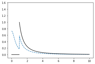
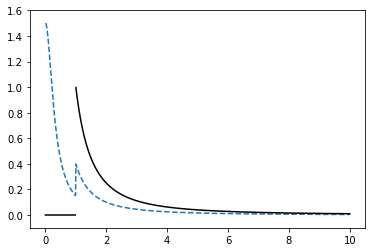
Figure 1: The dashed line is the probability density function of TT, the solid line is the probability density function of T0T_{0}. The left panel illustrates the case c=5c=5, and the right panel illustrates the case c=15c=15.

The random times

T=sup{u:η(u)=},T0=inf{u:η(u)=0},T=\sup\{u:\eta(u)=\infty\},\quad T_{0}=\operatorname*{\vphantom{p}inf}\{u:\eta(u)=0\},

are major characteristics of a trajectory of the limit pure death process. Since

P(Ty)=E(zη(y))|z=1,P(T0y)=E(zη(y))|z=0,\displaystyle\mathrm{P}(T\leq y)=\mathrm{E}(z^{\eta(y)})\Big{|}_{z=1},\qquad\mathrm{P}(T_{0}\leq y)=\mathrm{E}(z^{\eta(y)})\Big{|}_{z=0},

in accordance with the above mentioned formulas for E(zη(y))\mathrm{E}(z^{\eta(y)}), we get the following marginal distributions

P(Ty)\displaystyle\mathrm{P}(T\leq y) =1+cy21(1+1+c)y1{0y<1}+(12(1+1+c)y)1{y1},\displaystyle=\frac{\sqrt{1+cy^{2}}-1}{(1+\sqrt{1+c})y}\cdot 1_{\{0\leq y<1\}}+\Big{(}1-\frac{2}{(1+\sqrt{1+c})y}\Big{)}\cdot 1_{\{y\geq 1\}},
P(T0y)\displaystyle\mathrm{P}(T_{0}\leq y) =y1y1{y1}.\displaystyle=\frac{y-1}{y}\cdot 1_{\{y\geq 1\}}.

The distribution of T0T_{0} is free from the parameter cc and has the Pareto probability density function

f0(y)=y21{y>1}.f_{0}(y)=y^{-2}1_{\{y>1\}}.

In the special case (1.2), that is when (1.3) holds with d=0d=0, we have c=0c=0 and P(T=T0)=1\mathrm{P}(T=T_{0})=1. If d>0d>0, then TT0T\leq T_{0}, and the distribution of TT has the following probability density function

f(y)={1(1+1+c)y2(111+cy2)for0y<1,2(1+1+c)y2fory1,f(y)=\left\{\begin{array}[]{llr}\frac{1}{(1+\sqrt{1+c})y^{2}}(1-\frac{1}{\sqrt{1+cy^{2}}})&\text{for}&0\leq y<1,\\ \frac{2}{(1+\sqrt{1+c})y^{2}}&\text{for}&y\geq 1,\end{array}\right.

having a positive jump at y=1y=1 of size f(1)f(1)=(1+c)1/2f(1)-f(1-)=(1+c)^{-1/2}. Observe that f(1)f(1)12\frac{f(1-)}{f(1)}\to\frac{1}{2} as cc\to\infty.

Intuitively, the limiting pure death process counts the long-living individuals in the GWO-process, that is those individuals whose life length is of order tt. These long-living individuals may have descendants, however none of them would live long enough to be detected by the finite dimensional distributions at the relevant time scale, see Lemma 2 below. Theorem 1 suggests a new perspective on Vatutin’s dichotomy, see [12], claiming that the long term survival of a critical age-dependent branching process is due to either a large number of short-living individuals or a small number of long-living individuals. In terms of the random times TT0T\leq T_{0}, Vatutin’s dichotomy discriminates between two possibilities: if T>1T>1, then η(1)=\eta(1)=\infty, meaning that the GWO-process has survived due to a large number of individuals, while if T1<T0T\leq 1<T_{0}, then 1η(1)<1\leq\eta(1)<\infty meaning that the GWO-process has survived due to a small number of individuals.

3 Proof of  𝒕𝑸(𝒕)𝒉\boldsymbol{tQ(t)\to h}

This section deals with the survival probability of the critical GWO-process

Q(t)=1P(t),P(t):=P(Z(t)=0).Q(t)=1-P(t),\quad P(t):=\mathrm{P}(Z(t)=0).

By its definition, the GWO-process can be represented as the sum

Z(t)=1{L>t}+j=1NZj(tτj),t=0,1,,Z(t)=1_{\{L>t\}}+\sum\nolimits_{j=1}^{N}Z_{j}(t-\tau_{j}),\quad t=0,1,\ldots, (3.1)

involving NN independent daughter processes Zj()Z_{j}(\cdot) generated by the founder individual at the birth times τj\tau_{j}, j=1,,Nj=1,\ldots,N (here it is assumed that Zj(t)=0Z_{j}(t)=0 for all negative tt). The branching property (3.1) implies the relation

1{Z(t)=0}=1{Lt}j=1N1{Zj(tτj)=0},1_{\{Z(t)=0\}}=1_{\{L\leq t\}}\prod\nolimits_{j=1}^{N}1_{\{Z_{j}(t-\tau_{j})=0\}},

saying that the GWO-process goes extinct by the time tt if, on one hand, the founder is dead at time tt and, on the other hand, all daughter processes are extinct by the time tt. After taking expectations of both sides, we can write

P(t)=E(j=1NP(tτj);Lt).P(t)=\mathrm{E}\Big{(}\prod\nolimits_{j=1}^{N}P(t-\tau_{j});L\leq t\Big{)}. (3.2)

As shown next, this non-linear equation for P()P(\cdot) entails the asymptotic formula (1.4) under conditions (1.1), (1.3), and a<a<\infty.

3.1 Outline of the proof of (1.4)

We start by stating four lemmas and two propositions. Let

Φ(z)\displaystyle\Phi(z) :=E((1z)N1+Nz),\displaystyle:=\mathrm{E}((1-z)^{N}-1+Nz), (3.3)
W(t)\displaystyle W(t) :=(1ht1)N+Nht1j=1NQ(tτj)j=1NP(tτj),\displaystyle:=(1-ht^{-1})^{N}+Nht^{-1}-\sum\nolimits_{j=1}^{N}Q(t-\tau_{j})-\prod\nolimits_{j=1}^{N}P(t-\tau_{j}), (3.4)
D(u,t)\displaystyle D(u,t) :=E(1j=1NP(tτj);u<Lt)+E((1ht1)N1+Nht1;L>u),\displaystyle:=\mathrm{E}\Big{(}1-\prod\nolimits_{j=1}^{N}P(t-\tau_{j});\,u<L\leq t\Big{)}+\mathrm{E}\Big{(}(1-ht^{-1})^{N}-1+Nht^{-1};L>u\Big{)}, (3.5)
Eu(X)\displaystyle\mathrm{E}_{u}(X) :=E(X;Lu),\displaystyle:=\mathrm{E}(X;L\leq u), (3.6)

where 0z10\leq z\leq 1, u>0u>0, tht\geq h, and XX is an arbitrary random variable.

Lemma 1.

Given (3.3), (3.4), (3.5), and (3.6), assume that 0<ut0<u\leq t and tht\geq h. Then

Φ(ht1)=P(L>t)+Eu(j=1NQ(tτj))Q(t)+Eu(W(t))+D(u,t).\displaystyle\Phi(ht^{-1})=\mathrm{P}(L>t)+\mathrm{E}_{u}\Big{(}\sum\nolimits_{j=1}^{N}Q(t-\tau_{j})\Big{)}-Q(t)+\mathrm{E}_{u}(W(t))+D(u,t).

Lemma 2.

If (1.1) and (1.3) hold, then E(N;L>ty)=o(t1)\mathrm{E}(N;L>ty)=o(t^{-1}) as tt\to\infty for any fixed y>0y>0.

Lemma 3.

If (1.1), (1.3), and a<a<\infty hold, then for any fixed 0<y<10<y<1,

Ety(j=1N(1tτj1t))at2,t.\displaystyle\mathrm{E}_{ty}\Big{(}\sum\nolimits_{j=1}^{N}\Big{(}\frac{1}{t-\tau_{j}}-\frac{1}{t}\Big{)}\Big{)}\sim at^{-2},\quad t\to\infty.

Lemma 4.

Let k1k\geq 1. If 0fj,gj10\leq f_{j},g_{j}\leq 1 for j=1,,kj=1,\ldots,k, then

j=1k(1gj)j=1k(1fj)=j=1k(fjgj)rj,\prod\nolimits_{j=1}^{k}(1-g_{j})-\prod\nolimits_{j=1}^{k}(1-f_{j})=\sum\nolimits_{j=1}^{k}(f_{j}-g_{j})r_{j},

where 0rj10\leq r_{j}\leq 1 and

1rj=i=1j1gi+i=j+1kfiRj,\displaystyle 1-r_{j}=\sum\nolimits_{i=1}^{j-1}g_{i}+\sum\nolimits_{i=j+1}^{k}f_{i}-R_{j},

for some Rj0R_{j}\geq 0. If moreover, fjqf_{j}\leq q and gjqg_{j}\leq q for some q>0q>0, then

1rj(k1)q,Rjkq,Rjk2q2.1-r_{j}\leq(k-1)q,\qquad R_{j}\leq kq,\qquad R_{j}\leq k^{2}q^{2}.

Proposition 1.

If (1.1), (1.3), and a<a<\infty hold, then lim supttQ(t)<\limsup_{t\to\infty}tQ(t)<\infty.

Proposition 2.

If (1.1), (1.3), and a<a<\infty hold, then liminfttQ(t)>0\operatorname*{\vphantom{p}liminf}_{t\to\infty}tQ(t)>0.

According to these two propositions, there exists a triplet of positive numbers (q1,q2,t0)(q_{1},q_{2},t_{0}) such that

q1tQ(t)q2,tt0,0<q1<h<q2<.q_{1}\leq tQ(t)\leq q_{2},\quad t\geq t_{0},\quad 0<q_{1}<h<q_{2}<\infty. (3.7)

The claim tQ(t)htQ(t)\to h is derived using (3.7) by accurately removing asymptotically negligible terms from the relation for Q()Q(\cdot) stated in Lemma 1, after setting u=tyu=ty with a fixed 0<y<10<y<1, and then choosing a sufficiently small yy. In particular, as an intermediate step, we will show that

Q(t)=Ety(j=1NQ(tτj))+Ety(W(t))aht2+o(t2),t.\displaystyle Q(t)=\mathrm{E}_{ty}\Big{(}\sum\nolimits_{j=1}^{N}Q(t-\tau_{j})\Big{)}+\mathrm{E}_{ty}(W(t))-aht^{-2}+o(t^{-2}),\quad t\to\infty. (3.8)

Then, restating our goal as ϕ(t)0\phi(t)\to 0 in terms of the function ϕ(t)\phi(t), defined by

Q(t)=h+ϕ(t)t,t1,Q(t)=\frac{h+\phi(t)}{t},\quad t\geq 1, (3.9)

we rewrite (3.8) as

h+ϕ(t)t\displaystyle\frac{h+\phi(t)}{t} =Ety(j=1Nh+ϕ(tτj)tτj)+Ety(W(t))aht2+o(t2),t.\displaystyle=\mathrm{E}_{ty}\Big{(}\sum\nolimits_{j=1}^{N}\frac{h+\phi(t-\tau_{j})}{t-\tau_{j}}\Big{)}+\mathrm{E}_{ty}(W(t))-aht^{-2}+o(t^{-2}),\quad t\to\infty. (3.10)

It turns out that the three terms involving hh, outside W(t)W(t), effectively cancel each other, yielding

ϕ(t)t\displaystyle\frac{\phi(t)}{t} =Ety(j=1Nϕ(tτj)tτj+W(t))+o(t2),t.\displaystyle=\mathrm{E}_{ty}\Big{(}\sum\nolimits_{j=1}^{N}\frac{\phi(t-\tau_{j})}{t-\tau_{j}}+W(t)\Big{)}+o(t^{-2}),\quad t\to\infty. (3.11)

Treating W(t)W(t) in terms of Lemma 4, brings

ϕ(t)\displaystyle\phi(t) =Ety(j=1Nϕ(tτj)rj(t)ttτj)+o(t1),\displaystyle=\mathrm{E}_{ty}\Big{(}\sum\nolimits_{j=1}^{N}\phi(t-\tau_{j})r_{j}(t)\frac{t}{t-\tau_{j}}\Big{)}+o(t^{-1}), (3.12)

where rj(t)r_{j}(t) is a counterpart of rjr_{j} in Lemma 4. To derive from here the desired convergence ϕ(t)0\phi(t)\to 0, we will adapt a clever trick from Chapter 9.1 of [10], which was further developed in [12] for the Bellman-Harris process, with possibly infinite Var(N)\mathrm{Var\hskip 0.56905pt}(N). Define a non-negative function m(t)m(t) by

m(t):=|ϕ(t)|lnt,t2.\displaystyle m(t):=|\phi(t)|\,\ln t,\quad t\geq 2. (3.13)

Multiplying (3.12) by lnt\ln t and using the triangle inequality, we obtain

m(t)Ety(j=1Nm(tτj)rj(t)tlnt(tτj)ln(tτj))+v(t),\displaystyle m(t)\leq\mathrm{E}_{ty}\Big{(}\sum\nolimits_{j=1}^{N}m(t-\tau_{j})r_{j}(t)\frac{t\ln t}{(t-\tau_{j})\ln(t-\tau_{j})}\Big{)}+v(t), (3.14)

where v(t)0v(t)\geq 0 and v(t)=o(t1lnt)v(t)=o(t^{-1}\ln t) as tt\to\infty. It will be shown that this leads to m(t)=o(lnt)m(t)=o(\ln t), thereby concluding the proof of (1.4).

3.2 Proof of lemmas and propositions

Proof.

of Lemma 1. For 0<ut0<u\leq t, relations (3.2) and (3.6) give

P(t)=Eu(j=1NP(tτj))+E(j=1NP(tτj);u<Lt).\displaystyle P(t)=\mathrm{E}_{u}\Big{(}\prod\nolimits_{j=1}^{N}P(t-\tau_{j})\Big{)}+\mathrm{E}\Big{(}\prod\nolimits_{j=1}^{N}P(t-\tau_{j});u<L\leq t\Big{)}. (3.15)

On the other hand, for tht\geq h,

Φ(ht1)\displaystyle\Phi(ht^{-1}) =(3.3)Eu((1ht1)N1+Nht1)+E((1ht1)N1+Nht1;L>u).\displaystyle\stackrel{{\scriptstyle\eqref{AL}}}{{=}}\mathrm{E}_{u}\Big{(}(1-ht^{-1})^{N}-1+Nht^{-1}\Big{)}+\mathrm{E}\Big{(}(1-ht^{-1})^{N}-1+Nht^{-1};L>u\Big{)}.

Adding the latter relation to

1\displaystyle 1 =P(Lu)+P(L>t)+P(u<Lt),\displaystyle=\mathrm{P}(L\leq u)+\mathrm{P}(L>t)+\mathrm{P}(u<L\leq t),

and subtracting (3.15) from the sum, we get

Φ(ht1)+Q(t)=Eu((1ht1)N+Nht1j=1NP(tτj))+P(L>t)+D(u,t),\displaystyle\Phi(ht^{-1})+Q(t)=\mathrm{E}_{u}\Big{(}(1-ht^{-1})^{N}+Nht^{-1}-\prod\nolimits_{j=1}^{N}P(t-\tau_{j})\Big{)}+\mathrm{P}(L>t)+D(u,t),

with D(u,t)D(u,t) defined by (3.5). After a rearrangement, we obtain the statement of the lemma.

Proof.

of Lemma 2. For any fixed ϵ>0\epsilon>0,

E(N;L>t)=E(N;Ntϵ,L>t)+E(N;1<N(tϵ)1,L>t)tϵP(L>t)+(tϵ)1E(N2;L>t).\displaystyle\mathrm{E}(N;L>t)=\mathrm{E}(N;N\leq t\epsilon,L>t)+\mathrm{E}(N;1<N(t\epsilon)^{-1},L>t)\leq t\epsilon\mathrm{P}(L>t)+(t\epsilon)^{-1}\mathrm{E}(N^{2};L>t).

Thus, by (1.1) and (1.3),

lim supt(tE(N;L>t))dϵ,\displaystyle\limsup_{t\to\infty}(t\mathrm{E}(N;L>t))\leq d\epsilon,

and the assertion follows as ϵ0\epsilon\to 0.

Proof.

of Lemma 3. For t=1,2,t=1,2,\ldots and y>0y>0, put

Bt(y)\displaystyle B_{t}(y) :=t2Ety(j=1N(1tτj1t))a.\displaystyle:=t^{2}\,\mathrm{E}_{ty}\Big{(}\sum\nolimits_{j=1}^{N}\Big{(}\frac{1}{t-\tau_{j}}-\frac{1}{t}\Big{)}\Big{)}-a.

For any 0<u<ty0<u<ty, using

a=Eu(τ1++τN)+Au,Au:=E(τ1++τN;L>u),a=\mathrm{E}_{u}(\tau_{1}+\ldots+\tau_{N})+A_{u},\quad A_{u}:=\mathrm{E}(\tau_{1}+\ldots+\tau_{N};L>u),

we get

Bt(y)\displaystyle B_{t}(y) =Eu(j=1Nttτjτj)+E(j=1Nttτjτj;u<Lty)Eu(τ1++τN)Au\displaystyle=\mathrm{E}_{u}\Big{(}\sum\nolimits_{j=1}^{N}\frac{t}{t-\tau_{j}}\tau_{j}\Big{)}+\mathrm{E}\Big{(}\sum\nolimits_{j=1}^{N}\frac{t}{t-\tau_{j}}\tau_{j}\,;u<L\leq ty\Big{)}-\mathrm{E}_{u}(\tau_{1}+\ldots+\tau_{N})-A_{u}
=E(j=1Nτj1τj/t;u<Lty)+Eu(j=1Nτj2tτj)Au.\displaystyle=\mathrm{E}\Big{(}\sum\nolimits_{j=1}^{N}\frac{\tau_{j}}{1-\tau_{j}/t};u<L\leq ty\Big{)}+\mathrm{E}_{u}\Big{(}\sum\nolimits_{j=1}^{N}\frac{\tau_{j}^{2}}{t-\tau_{j}}\Big{)}-A_{u}.

For the first term on the right hand side, we have τjLty\tau_{j}\leq L\leq ty, so that

E(j=1Nτj1τj/t;u<Lty)(1y)1Au.\displaystyle\mathrm{E}\Big{(}\sum\nolimits_{j=1}^{N}\frac{\tau_{j}}{1-\tau_{j}/t};u<L\leq ty\Big{)}\leq(1-y)^{-1}A_{u}.

For the second term, τjLu\tau_{j}\leq L\leq u and therefore

Eu(j=1Nτj2tτj)u2tuEu(N)u2tu.\displaystyle\mathrm{E}_{u}\Big{(}\sum\nolimits_{j=1}^{N}\frac{\tau_{j}^{2}}{t-\tau_{j}}\Big{)}\leq\frac{u^{2}}{t-u}\mathrm{E}_{u}(N)\leq\frac{u^{2}}{t-u}.

This yields

AuBt(y)(1y)1Au+u2tu,0<u<ty<t,-A_{u}\leq B_{t}(y)\leq(1-y)^{-1}A_{u}+\frac{u^{2}}{t-u},\quad 0<u<ty<t,

implying

AuliminftBt(y)lim suptBt(y)(1y)1Au.-A_{u}\leq\operatorname*{\vphantom{p}liminf}_{t\to\infty}B_{t}(y)\leq\limsup_{t\to\infty}B_{t}(y)\leq(1-y)^{-1}A_{u}.

Since Au0A_{u}\to 0 as uu\to\infty, we conclude that Bt0B_{t}\to 0 as tt\to\infty.

Proof.

of Lemma 4. Let

rj:=(1g1)(1gj1)(1fj+1)(1fk),1jk.r_{j}:=(1-g_{1})\ldots(1-g_{j-1})(1-f_{j+1})\ldots(1-f_{k}),\quad 1\leq j\leq k.

Then 0rj10\leq r_{j}\leq 1 and the first stated equality is obtained by telescopic summation of

(1g1)j=2k(1fj)j=1k(1fj)\displaystyle(1-g_{1})\prod\nolimits_{j=2}^{k}(1-f_{j})-\prod\nolimits_{j=1}^{k}(1-f_{j}) =(f1g1)r1,\displaystyle=(f_{1}-g_{1})r_{1},
(1g1)(1g2)j=3k(1fj)(1g1)j=2k(1fj)\displaystyle(1-g_{1})(1-g_{2})\prod\nolimits_{j=3}^{k}(1-f_{j})-(1-g_{1})\prod\nolimits_{j=2}^{k}(1-f_{j}) =(f2g2)r2,,\displaystyle=(f_{2}-g_{2})r_{2},\ldots,
j=1k(1gj)j=1k1(1gj)(1fk)\displaystyle\prod\nolimits_{j=1}^{k}(1-g_{j})-\prod\nolimits_{j=1}^{k-1}(1-g_{j})(1-f_{k}) =(fkgk)rk.\displaystyle=(f_{k}-g_{k})r_{k}.

The second stated equality is obtained with

Rj\displaystyle R_{j} :=i=j+1kfi(1(1fj+1)(1fi1))+i=1j1gi(1(1g1)(1gi1)(1fj+1)(1fk)),\displaystyle:=\sum_{i=j+1}^{k}f_{i}(1-(1-f_{j+1})\ldots(1-f_{i-1}))+\sum_{i=1}^{j-1}g_{i}(1-(1-g_{1})\ldots(1-g_{i-1})(1-f_{j+1})\ldots(1-f_{k})),

by performing telescopic summation of

1(1fj+1)\displaystyle 1-(1-f_{j+1}) =fj+1,\displaystyle=f_{j+1},
(1fj+1)(1fj+1)(1fj+2)\displaystyle(1-f_{j+1})-(1-f_{j+1})(1-f_{j+2}) =fj+2(1fj+1),,\displaystyle=f_{j+2}(1-f_{j+1}),\ldots,
i=j+1k1(1fi)i=j+1k(1fi)\displaystyle\prod\nolimits_{i=j+1}^{k-1}(1-f_{i})-\prod\nolimits_{i=j+1}^{k}(1-f_{i}) =fki=j+1k1(1fi),\displaystyle=f_{k}\prod\nolimits_{i=j+1}^{k-1}(1-f_{i}),
i=j+1k(1fi)(1g1)i=j+1k(1fi)\displaystyle\prod\nolimits_{i=j+1}^{k}(1-f_{i})-(1-g_{1})\prod\nolimits_{i=j+1}^{k}(1-f_{i}) =g1i=j+1k(1fi),,\displaystyle=g_{1}\prod\nolimits_{i=j+1}^{k}(1-f_{i}),\ldots,
i=1j2(1gi)i=j+1k(1fi)i=1j1(1gi)i=j+1k(1fi)\displaystyle\prod\nolimits_{i=1}^{j-2}(1-g_{i})\prod\nolimits_{i=j+1}^{k}(1-f_{i})-\prod\nolimits_{i=1}^{j-1}(1-g_{i})\prod\nolimits_{i=j+1}^{k}(1-f_{i}) =gj1i=1j2(1gi)i=j+1k(1fi).\displaystyle=g_{j-1}\prod\nolimits_{i=1}^{j-2}(1-g_{i})\prod\nolimits_{i=j+1}^{k}(1-f_{i}).

By the above definition of RjR_{j}, we have Rj0R_{j}\geq 0. Furthermore, given fjqf_{j}\leq q and gjqg_{j}\leq q, we get

Rji=1j1gi+i=j+1kfi(k1)q.R_{j}\leq\sum\nolimits_{i=1}^{j-1}g_{i}+\sum\nolimits_{i=j+1}^{k}f_{i}\leq(k-1)q.

It remains to observe that

1rj1(1q)k1(k1)q,\displaystyle 1-r_{j}\leq 1-(1-q)^{k-1}\leq(k-1)q,

and from the definition of RjR_{j},

Rjqi=1kj1(1(1q)i)+qi=1j1(1(1q)kj+i1)q2i=1k2ik2q2.R_{j}\leq q\sum\nolimits_{i=1}^{k-j-1}(1-(1-q)^{i})+q\sum\nolimits_{i=1}^{j-1}(1-(1-q)^{k-j+i-1})\leq q^{2}\sum\nolimits_{i=1}^{k-2}i\leq k^{2}q^{2}.

Proof.

of Proposition 1. By the definition of Φ()\Phi(\cdot), we have

Φ(Q(t))+P(t)=Eu(P(t)N)+P(L>u)E(1P(t)N;L>u),\Phi(Q(t))+P(t)=\mathrm{E}_{u}\Big{(}P(t)^{N}\Big{)}+\mathrm{P}(L>u)-\mathrm{E}\Big{(}1-P(t)^{N};\,L>u\Big{)},

for any 0<u<t0<u<t. This and (3.15) yield

Φ(Q(t))\displaystyle\Phi(Q(t)) =Eu(P(t)Nj=1NP(tτj))+P(L>u)\displaystyle=\mathrm{E}_{u}\Big{(}P(t)^{N}-\prod\nolimits_{j=1}^{N}P(t-\tau_{j})\Big{)}+\mathrm{P}(L>u)
E(1P(t)N;L>u)E(j=1NP(tτj);u<Lt).\displaystyle-\mathrm{E}\Big{(}1-P(t)^{N};\,L>u\Big{)}-\mathrm{E}\Big{(}\prod\nolimits_{j=1}^{N}P(t-\tau_{j});u<L\leq t\Big{)}. (3.16)

An upper bound follows

Φ(Q(t))\displaystyle\Phi(Q(t)) Eu(P(t)Nj=1NP(tτj))+P(L>u),\displaystyle\leq\mathrm{E}_{u}\Big{(}P(t)^{N}-\prod\nolimits_{j=1}^{N}P(t-\tau_{j})\Big{)}+\mathrm{P}(L>u),

which together with Lemma 4 and monotonicity of Q()Q(\cdot) entail

Φ(Q(t))Eu(j=1N(Q(tτj)Q(t)))+P(L>u).\displaystyle\Phi(Q(t))\leq\mathrm{E}_{u}\Big{(}\sum\nolimits_{j=1}^{N}(Q(t-\tau_{j})-Q(t))\Big{)}+\mathrm{P}(L>u). (3.17)

Borrowing an idea from [11], suppose, on the contrary, that

tn:=min{t:tQ(t)n}t_{n}:=\min\{t:tQ(t)\geq n\}

is finite for any natural nn. It follows that

Q(tn)ntn,Q(tnu)<ntnu,1utn1.Q(t_{n})\geq\frac{n}{t_{n}},\qquad Q(t_{n}-u)<\frac{n}{t_{n}-u},\quad 1\leq u\leq t_{n}-1.

Putting t=tnt=t_{n} into (3.17) and using monotonicity of Φ()\Phi(\cdot), we find

Φ(ntn1)Φ(Q(tn))Eu(j=1N(ntnτjntn))+P(L>u).\displaystyle\Phi(nt_{n}^{-1})\leq\Phi(Q(t_{n}))\leq\mathrm{E}_{u}\Big{(}\sum\nolimits_{j=1}^{N}\Big{(}\frac{n}{t_{n}-\tau_{j}}-\frac{n}{t_{n}}\Big{)}\Big{)}+\mathrm{P}(L>u).

Setting here u=tn/2u=t_{n}/2 and applying Lemma 3 together with (1.3), we arrive at the relation

Φ(ntn1)=O(ntn2),n.\Phi(nt_{n}^{-1})=O(nt_{n}^{-2}),\quad n\to\infty.

Observe that under condition (1.1), the L’Hospital rule gives

Φ(z)bz2,z0.\Phi(z)\sim bz^{2},\quad z\to 0. (3.18)

The resulting contradiction, n2tn2=O(ntn2)n^{2}t_{n}^{-2}=O(nt_{n}^{-2}) as nn\to\infty, finishes the proof of the proposition.

Proof.

of Proposition 2. Relation (3.16) implies

Φ(Q(t))Eu(P(t)Nj=1NP(tτj))E(1P(t)N;L>u).\displaystyle\Phi(Q(t))\geq\mathrm{E}_{u}\Big{(}P(t)^{N}-\prod\nolimits_{j=1}^{N}P(t-\tau_{j})\Big{)}-\mathrm{E}\Big{(}1-P(t)^{N};\,L>u\Big{)}.

By Lemma 4,

P(t)Nj=1NP(tτj)=j=1N(Q(tτj)Q(t))rj(t),\displaystyle P(t)^{N}-\prod\nolimits_{j=1}^{N}P(t-\tau_{j})=\sum_{j=1}^{N}(Q(t-\tau_{j})-Q(t))r_{j}^{*}(t),

where 0rj(t)10\leq r_{j}^{*}(t)\leq 1 is a counterpart of term rjr_{j} in Lemma 4. Due to monotonicity of P()P(\cdot), we have, again referring to Lemma 4,

1rj(t)(N1)Q(tL).1-r_{j}^{*}(t)\leq(N-1)Q(t-L).

Thus, for 0<y<10<y<1,

Φ(Q(t))\displaystyle\Phi(Q(t)) Ety(j=1N(Q(tτj)Q(t))rj(t))E(1P(t)N;L>ty).\displaystyle\geq\mathrm{E}_{ty}\Big{(}\sum_{j=1}^{N}(Q(t-\tau_{j})-Q(t))r_{j}^{*}(t)\Big{)}-\mathrm{E}\Big{(}1-P(t)^{N};\,L>ty\Big{)}. (3.19)

The assertion liminfttQ(t)>0\operatorname*{\vphantom{p}liminf}_{t\to\infty}tQ(t)>0 is proven by contradiction. Assume that liminfttQ(t)=0\operatorname*{\vphantom{p}liminf}_{t\to\infty}tQ(t)=0, so that

tn:=min{t:tQ(t)n1}t_{n}:=\min\{t:tQ(t)\leq n^{-1}\}

is finite for any natural nn. Plugging t=tnt=t_{n} in (3.19) and using

Q(tn)1ntn,Q(tnu)Q(tn)1n(tnu)1ntn,1utn1,Q(t_{n})\leq\frac{1}{nt_{n}},\quad Q(t_{n}-u)-Q(t_{n})\geq\frac{1}{n(t_{n}-u)}-\frac{1}{nt_{n}},\quad 1\leq u\leq t_{n}-1,

we get

Φ(1ntn)n1Etny(j=1N(1tnτj1tn)rj(tn))1ntnE(N;L>tny).\Phi\Big{(}\frac{1}{nt_{n}}\Big{)}\geq n^{-1}\mathrm{E}_{t_{n}y}\Big{(}\sum\nolimits_{j=1}^{N}\Big{(}\frac{1}{t_{n}-\tau_{j}}-\frac{1}{t_{n}}\Big{)}r_{j}^{*}(t_{n})\Big{)}-\frac{1}{nt_{n}}\mathrm{E}(N;\,L>t_{n}y).

Given LtyL\leq ty, we have

1rj(t)NQ(t(1y))Nq2t(1y),\displaystyle 1-r_{j}^{*}(t)\leq NQ(t(1-y))\leq N\frac{q_{2}}{t(1-y)},

where the second inequality is based on the already proven part of (3.7). Therefore,

Etny(j=1N(1tnτj1tn)(1rj(tn)))q2ytn2(1y)2E(N2),\mathrm{E}_{t_{n}y}\Big{(}\sum\nolimits_{j=1}^{N}\Big{(}\frac{1}{t_{n}-\tau_{j}}-\frac{1}{t_{n}}\Big{)}(1-r_{j}^{*}(t_{n}))\Big{)}\leq\frac{q_{2}y}{t_{n}^{2}(1-y)^{2}}\mathrm{E}(N^{2}),

and we derive

ntn2Φ(1ntn)\displaystyle nt_{n}^{2}\Phi(\tfrac{1}{nt_{n}}) tn2Etny(j=1N(1tnτj1tn))E(N2)q2y(1y)2tnE(N;L>tny).\displaystyle\geq t_{n}^{2}\mathrm{E}_{t_{n}y}\Big{(}\sum\nolimits_{j=1}^{N}\Big{(}\frac{1}{t_{n}-\tau_{j}}-\frac{1}{t_{n}}\Big{)}\Big{)}-\frac{\mathrm{E}(N^{2})q_{2}y}{(1-y)^{2}}-t_{n}\mathrm{E}(N;\,L>t_{n}y).

Sending nn\to\infty and applying (3.18), Lemma 2, and Lemma 3, we arrive at the inequality

0ayq2E(N2)(1y)2,0<y<1,0\geq a-yq_{2}\mathrm{E}(N^{2})(1-y)^{-2},\quad 0<y<1,

which is false for sufficiently small yy.

3.3 Proof of (3.11) and (3.12)

Fix an arbitrary 0<y<10<y<1. Lemma 1 with u=tyu=ty, gives

Φ(ht1)=P(L>t)+Ety(j=1NQ(tτj))Q(t)+Ety(W(t))+D(ty,t).\displaystyle\Phi(ht^{-1})=\mathrm{P}(L>t)+\mathrm{E}_{ty}\Big{(}\sum\nolimits_{j=1}^{N}Q(t-\tau_{j})\Big{)}-Q(t)+\mathrm{E}_{ty}(W(t))+D(ty,t). (3.20)

Let us show that

D(ty,t)=o(t2),t.\displaystyle D(ty,t)=o(t^{-2}),\quad t\to\infty. (3.21)

Using Lemma 2 and (3.7), we find that for an arbitrarily small ϵ>0\epsilon>0,

E(1j=1NP(tτj);ty<Lt(1ϵ))=o(t2),t.\mathrm{E}\Big{(}1-\prod\nolimits_{j=1}^{N}P(t-\tau_{j});\,ty<L\leq t(1-\epsilon)\Big{)}=o(t^{-2}),\quad t\to\infty.

On the other hand,

E(1j=1NP(tτj);t(1ϵ)<Lt)P(t(1ϵ)<Lt),\displaystyle\mathrm{E}\Big{(}1-\prod\nolimits_{j=1}^{N}P(t-\tau_{j});\,t(1-\epsilon)<L\leq t\Big{)}\leq\mathrm{P}(t(1-\epsilon)<L\leq t),

so that in view of (1.3),

E(1j=1NP(tτj);ty<Lt)=o(t2),t.\mathrm{E}\Big{(}1-\prod\nolimits_{j=1}^{N}P(t-\tau_{j});\,ty<L\leq t\Big{)}=o(t^{-2}),\quad t\to\infty.

This, (3.5) and Lemma 2 entail (3.21).

Observe that

bh2=ah+d.bh^{2}=ah+d. (3.22)

Combining (3.20), (3.21), and

P(L>t)Φ(ht1)=(1.3)(3.18)dt2bh2t2+o(t2)=(3.22)aht2+o(t2),t,\mathrm{P}(L>t)-\Phi(ht^{-1})\stackrel{{\scriptstyle\eqref{d}\eqref{L1}}}{{=}}dt^{-2}-bh^{2}t^{-2}+o(t^{-2})\stackrel{{\scriptstyle\eqref{stop}}}{{=}}-aht^{-2}+o(t^{-2}),\quad t\to\infty,

we derive (3.8), which in turn gives (3.10). The latter implies (3.11) since by Lemmas 2 and 4,

Ety(j=1Nhtτj)ht=Ety(j=1N(htτjht))ht1E(N;L>ty)=aht2+o(t2).\mathrm{E}_{ty}\Big{(}\sum\nolimits_{j=1}^{N}\frac{h}{t-\tau_{j}}\Big{)}-\frac{h}{t}=\mathrm{E}_{ty}\Big{(}\sum\nolimits_{j=1}^{N}\Big{(}\frac{h}{t-\tau_{j}}-\frac{h}{t}\Big{)}\Big{)}-ht^{-1}\mathrm{E}(N;L>ty)=aht^{-2}+o(t^{-2}).

Turning to the proof of (3.12), observe that the random variable

W(t)=(1ht1)Nj=1N(1h+ϕ(tτj)tτj)+j=1N(hth+ϕ(tτj)tτj),W(t)=(1-ht^{-1})^{N}-\prod\nolimits_{j=1}^{N}\Big{(}1-\frac{h+\phi(t-\tau_{j})}{t-\tau_{j}}\Big{)}+\sum\nolimits_{j=1}^{N}\Big{(}\frac{h}{t}-\frac{h+\phi(t-\tau_{j})}{t-\tau_{j}}\Big{)},

can be represented in terms of Lemma 4 as

W(t)=j=1N(1fj(t))j=1N(1gj(t))+j=1N(fj(t)gj(t))=j=1N(1rj(t))(fj(t)gj(t)),W(t)=\prod\nolimits_{j=1}^{N}(1-f_{j}(t))-\prod\nolimits_{j=1}^{N}(1-g_{j}(t))+\sum\nolimits_{j=1}^{N}(f_{j}(t)-g_{j}(t))=\sum\nolimits_{j=1}^{N}(1-r_{j}(t))(f_{j}(t)-g_{j}(t)),

by assigning

fj(t):=ht1,gj(t):=h+ϕ(tτj)tτj.\displaystyle f_{j}(t):=ht^{-1},\quad g_{j}(t):=\frac{h+\phi(t-\tau_{j})}{t-\tau_{j}}. (3.23)

Here 0rj(t)10\leq r_{j}(t)\leq 1 and for sufficiently large tt,

1rj(t)(3.7)Nq2t1.\displaystyle 1-r_{j}(t)\stackrel{{\scriptstyle\eqref{ca}}}{{\leq}}Nq_{2}t^{-1}. (3.24)

After plugging into (3.11) the expression

W(t)=j=1N(hthtτj)(1rj(t))j=1Nϕ(tτj)tτj(1rj(t)),W(t)=\sum\nolimits_{j=1}^{N}\Big{(}\frac{h}{t}-\frac{h}{t-\tau_{j}}\Big{)}(1-r_{j}(t))-\sum\nolimits_{j=1}^{N}\frac{\phi(t-\tau_{j})}{t-\tau_{j}}(1-r_{j}(t)),

we get

ϕ(t)t\displaystyle\frac{\phi(t)}{t} =Ety(j=1Nϕ(tτj)tτjrj(t))+Ety(j=1N(htτjht)(1rj(t)))+o(t2),t.\displaystyle=\mathrm{E}_{ty}\Big{(}\sum\nolimits_{j=1}^{N}\frac{\phi(t-\tau_{j})}{t-\tau_{j}}r_{j}(t)\Big{)}+\mathrm{E}_{ty}\Big{(}\sum\nolimits_{j=1}^{N}\Big{(}\frac{h}{t-\tau_{j}}-\frac{h}{t}\Big{)}(1-r_{j}(t))\Big{)}+o(t^{-2}),\quad t\to\infty.

The latter expectation is non-negative, and for an arbitrary ϵ>0\epsilon>0, it has the following upper bound

Ety(j=1N(htτjht)(1rj(t)))(3.24)q2ϵEty(j=1N(htτjht))+q2h(1y)t2E(N2;N>tϵ).\displaystyle\mathrm{E}_{ty}\Big{(}\sum\nolimits_{j=1}^{N}\Big{(}\frac{h}{t-\tau_{j}}-\frac{h}{t}\Big{)}(1-r_{j}(t))\Big{)}\stackrel{{\scriptstyle\eqref{stal}}}{{\leq}}q_{2}\epsilon\mathrm{E}_{ty}\Big{(}\sum\nolimits_{j=1}^{N}\Big{(}\frac{h}{t-\tau_{j}}-\frac{h}{t}\Big{)}\Big{)}+\frac{q_{2}h}{(1-y)t^{2}}\mathrm{E}(N^{2};N>t\epsilon).

Thus, in view of Lemma 3,

ϕ(t)t\displaystyle\frac{\phi(t)}{t} =Ety(j=1Nϕ(tτj)tτjrj(t))+o(t2),t.\displaystyle=\mathrm{E}_{ty}\Big{(}\sum\nolimits_{j=1}^{N}\frac{\phi(t-\tau_{j})}{t-\tau_{j}}r_{j}(t)\Big{)}+o(t^{-2}),\quad t\to\infty.

Multiplying this relation by tt, we arrive at (3.12).

3.4 Proof of ϕ(t)0\phi(t)\to 0

Recall (3.13). If the non-decreasing function

M(t):=max1jtm(j)M(t):=\operatorname*{\vphantom{p}max}_{1\leq j\leq t}m(j)

is bounded from above, then ϕ(t)=O(1lnt)\phi(t)=O(\frac{1}{\ln t}) proving that ϕ(t)0\phi(t)\to 0 as tt\to\infty. If M(t)M(t)\to\infty as tt\to\infty, then there is an integer-valued sequence 0<t1<t2<,0<t_{1}<t_{2}<\ldots, such that the sequence Mn:=M(tn)M_{n}:=M(t_{n}) is strictly increasing and converges to infinity. In this case,

m(t)Mn1<Mn,1t<tn,m(tn)=Mn,n1.m(t)\leq M_{n-1}<M_{n},\quad 1\leq t<t_{n},\quad m(t_{n})=M_{n},\quad n\geq 1. (3.25)

Since |ϕ(t)|Mnlntn|\phi(t)|\leq\frac{M_{n}}{\ln t_{n}} for tnt<tn+1t_{n}\leq t<t_{n+1}, to finish the proof of ϕ(t)0\phi(t)\to 0, it remains to verify that

Mn=o(lntn),n.M_{n}=o(\ln t_{n}),\quad n\to\infty. (3.26)

Fix an arbitrary y(0,1)y\in(0,1). Putting t=tnt=t_{n} in (3.14) and using (3.25), we find

MnMnEtny(j=1Nrj(tn)tnlntn(tnτj)ln(tnτj))+(tn1lntn)on.\displaystyle M_{n}\leq M_{n}\mathrm{E}_{t_{n}y}\Big{(}\sum\nolimits_{j=1}^{N}r_{j}(t_{n})\frac{t_{n}\ln t_{n}}{(t_{n}-\tau_{j})\ln(t_{n}-\tau_{j})}\Big{)}+(t_{n}^{-1}\ln t_{n})o_{n}.

Here and elsewhere, ono_{n} stands for a non-negative sequence such that on0o_{n}\to 0 as nn\to\infty. In different formulas, the sign ono_{n} represents different such sequences. Since

0tlnt(tu)ln(tu)1u(1+lnt)(tu)ln(tu),0u<t1,0\leq\frac{t\ln t}{(t-u)\ln(t-u)}-1\leq\frac{u(1+\ln t)}{(t-u)\ln(t-u)},\quad 0\leq u<t-1,

and rj(tn)[0,1]r_{j}(t_{n})\in[0,1], it follows that

MnMnEtny(j=1Nrj(tn))\displaystyle M_{n}-M_{n}\mathrm{E}_{t_{n}y}\Big{(}\sum\nolimits_{j=1}^{N}r_{j}(t_{n})\Big{)} MnEtny(j=1Nτj(1+lntn)tn(1y)ln(tn(1y)))+(tn1lntn)on.\displaystyle\leq M_{n}\mathrm{E}_{t_{n}y}\Big{(}\sum\nolimits_{j=1}^{N}\frac{\tau_{j}(1+\ln t_{n})}{t_{n}(1-y)\ln(t_{n}(1-y))}\Big{)}+(t_{n}^{-1}\ln t_{n})o_{n}.

Recalling that a=E(j=1Nτj)a=\mathrm{E}(\sum_{j=1}^{N}\tau_{j}), observe that

Etny(j=1Nτj(1+lntn)tn(1y)ln(tn(1y)))a(1+lntn)tn(1y)ln(tn(1y))=(a(1y)1+on)tn1.\displaystyle\mathrm{E}_{t_{n}y}\Big{(}\sum\nolimits_{j=1}^{N}\frac{\tau_{j}(1+\ln t_{n})}{t_{n}(1-y)\ln(t_{n}(1-y))}\Big{)}\leq\frac{a(1+\ln t_{n})}{t_{n}(1-y)\ln(t_{n}(1-y))}=(a(1-y)^{-1}+o_{n})t_{n}^{-1}.

Combining the last two relations, we conclude

MnEtny(j=1N(1rj(tn)))\displaystyle M_{n}\mathrm{E}_{t_{n}y}\Big{(}\sum\nolimits_{j=1}^{N}(1-r_{j}(t_{n}))\Big{)} a(1y)1tn1Mn+tn1(Mn+lntn)on.\displaystyle\leq a(1-y)^{-1}t_{n}^{-1}M_{n}+t_{n}^{-1}(M_{n}+\ln t_{n})o_{n}. (3.27)

Now it is time to unpack the term rj(t)r_{j}(t). By Lemma 4 with (3.23),

1rj(t)=i=1j1h+ϕ(tτi)tτi+(Nj)htRj(t),1-r_{j}(t)=\sum_{i=1}^{j-1}\frac{h+\phi(t-\tau_{i})}{t-\tau_{i}}+(N-j)\frac{h}{t}-R_{j}(t),

where provided τjty\tau_{j}\leq ty,

0Rj(t)Nq2t1(1y)1,Rj(t)N2q22t2(1y)2,t>t,0\leq R_{j}(t)\leq Nq_{2}t^{-1}(1-y)^{-1},\quad R_{j}(t)\leq N^{2}q_{2}^{2}t^{-2}(1-y)^{-2},\quad t>t^{*},

for a sufficiently large tt^{*}. This allows us to rewrite (3.27) in the form

MnEtny(j=1N\displaystyle M_{n}\mathrm{E}_{t_{n}y}\Big{(}\sum\nolimits_{j=1}^{N} (i=1j1h+ϕ(tnτi)tnτi+(Nj)htn))\displaystyle\Big{(}\sum_{i=1}^{j-1}\frac{h+\phi(t_{n}-\tau_{i})}{t_{n}-\tau_{i}}+(N-j)\frac{h}{t_{n}}\Big{)}\Big{)}
MnEtny(j=1NRj(tn))+a(1y)1tn1Mn+tn1(Mn+lntn)on.\displaystyle\leq M_{n}\mathrm{E}_{t_{n}y}\Big{(}\sum\nolimits_{j=1}^{N}R_{j}(t_{n})\Big{)}+a(1-y)^{-1}t_{n}^{-1}M_{n}+t_{n}^{-1}(M_{n}+\ln t_{n})o_{n}.

To estimate the last expectation, observe that if τjty\tau_{j}\leq ty, then for any ϵ>0\epsilon>0,

Rj(t)Nq2t1(1y)11{N>tϵ}+N2q22t2(1y)21{Ntϵ},t>t.R_{j}(t)\leq Nq_{2}t^{-1}(1-y)^{-1}1_{\{N>t\epsilon\}}+N^{2}q_{2}^{2}t^{-2}(1-y)^{-2}1_{\{N\leq t\epsilon\}},\quad t>t^{*}.

implying that for sufficiently large nn,

Etny(j=1NRj(tn))q2tn1(1y)1E(N2;N>tnϵ)+q22ϵtn1(1y)2E(N2),\mathrm{E}_{t_{n}y}\Big{(}\sum\nolimits_{j=1}^{N}R_{j}(t_{n})\Big{)}\leq q_{2}t_{n}^{-1}(1-y)^{-1}\mathrm{E}(N^{2};N>t_{n}\epsilon)+q_{2}^{2}\epsilon t_{n}^{-1}(1-y)^{-2}\mathrm{E}(N^{2}),

so that

MnEtny(j=1N(i=1j1h+ϕ(tnτi)tnτi+(Nj)htn))a(1y)1tn1Mn+tn1(Mn+lntn)on.\displaystyle M_{n}\mathrm{E}_{t_{n}y}\Big{(}\sum\nolimits_{j=1}^{N}\Big{(}\sum\nolimits_{i=1}^{j-1}\frac{h+\phi(t_{n}-\tau_{i})}{t_{n}-\tau_{i}}+(N-j)\frac{h}{t_{n}}\Big{)}\Big{)}\leq a(1-y)^{-1}t_{n}^{-1}M_{n}+t_{n}^{-1}(M_{n}+\ln t_{n})o_{n}.

Since

j=1Ni=1j1(htnτihtn)0,\sum\nolimits_{j=1}^{N}\sum\nolimits_{i=1}^{j-1}\Big{(}\frac{h}{t_{n}-\tau_{i}}-\frac{h}{t_{n}}\Big{)}\geq 0,

we obtain

MnEtny(j=1N(i=1j1ϕ(tnτi)tnτi+(N1)htn))a(1y)1tn1Mn+tn1(Mn+lntn)on.\displaystyle M_{n}\mathrm{E}_{t_{n}y}\Big{(}\sum\nolimits_{j=1}^{N}\Big{(}\sum_{i=1}^{j-1}\frac{\phi(t_{n}-\tau_{i})}{t_{n}-\tau_{i}}+(N-1)\frac{h}{t_{n}}\Big{)}\Big{)}\leq a(1-y)^{-1}t_{n}^{-1}M_{n}+t_{n}^{-1}(M_{n}+\ln t_{n})o_{n}.

By (3.9) and (3.7), we have ϕ(t)q1h\phi(t)\geq q_{1}-h for tt0t\geq t_{0}. Thus for τjLtny\tau_{j}\leq L\leq t_{n}y and sufficiently large nn,

ϕ(tnτi)tnτiq1htn(1y).\frac{\phi(t_{n}-\tau_{i})}{t_{n}-\tau_{i}}\stackrel{{\scriptstyle}}{{\geq}}\frac{q_{1}-h}{t_{n}(1-y)}.

This gives

j=1N(i=1j1ϕ(tnτi)tnτi+(N1)htn)(h+q1h2(1y))tn1N(N1),\sum\nolimits_{j=1}^{N}\Big{(}\sum_{i=1}^{j-1}\frac{\phi(t_{n}-\tau_{i})}{t_{n}-\tau_{i}}+(N-1)\frac{h}{t_{n}}\Big{)}\geq\Big{(}h+\frac{q_{1}-h}{2(1-y)}\Big{)}t_{n}^{-1}N(N-1),

which after multiplying by tnMnt_{n}M_{n} and taking expectations, yields

(h+q1h2(1y))MnEtny(N(N1))a(1y)1Mn+(Mn+lntn)on.\displaystyle\Big{(}h+\frac{q_{1}-h}{2(1-y)}\Big{)}M_{n}\mathrm{E}_{t_{n}y}(N(N-1))\leq a(1-y)^{-1}M_{n}+(M_{n}+\ln t_{n})o_{n}.

Finally, since

Etny(N(N1))2b,n,\mathrm{E}_{t_{n}y}(N(N-1))\to 2b,\quad n\to\infty,

we derive that for any 0<ϵ<y<10<\epsilon<y<1, there is a finite nϵn_{\epsilon} such that for all n>nϵn>n_{\epsilon},

Mn(2bh(1y)+bq1bhaϵ)ϵlntn.M_{n}\Big{(}2bh(1-y)+bq_{1}-bh-a-\epsilon\Big{)}\leq\epsilon\ln t_{n}.

By (3.22), we have bhabh\geq a, and therefore,

2bh(1y)+bq1bhaϵbq12bhyy.2bh(1-y)+bq_{1}-bh-a-\epsilon\geq bq_{1}-2bhy-y.

Thus, choosing y=y0y=y_{0} such that bq12bhy0y0=bq12bq_{1}-2bhy_{0}-y_{0}=\frac{bq_{1}}{2}, we see that

lim supnMnlntn2ϵbq1,\limsup_{n\to\infty}\frac{M_{n}}{\ln t_{n}}\leq\frac{2\epsilon}{bq_{1}},

which entails (3.26) as ϵ0\epsilon\to 0, concluding the proof of ϕ(t)0\phi(t)\to 0.

4 Proof of Theorem 1

We will use the following notational agreements for the kk-dimensional probability generating function

E(z1Z(t1)zkZ(tk))=i1=0ik=0P(Z(t1)=i1,,Z(tk)=ik)z1i1zkik,\mathrm{E}(z_{1}^{Z(t_{1})}\cdots z_{k}^{Z(t_{k})})=\sum_{i_{1}=0}^{\infty}\ldots\sum_{i_{k}=0}^{\infty}\mathrm{P}(Z(t_{1})=i_{1},\ldots,Z(t_{k})=i_{k})z_{1}^{i_{1}}\cdots z_{k}^{i_{k}},

with 0<t1tk0<t_{1}\leq\ldots\leq t_{k} and z1,,zk[0,1]z_{1},\ldots,z_{k}\in[0,1]. We denote

Pk(t¯,z¯):=Pk(t1,,tn;z1,,zk):=E(z1Z(t1)zkZ(tk)),P_{k}(\bar{t},\bar{z}):=P_{k}(t_{1},\ldots,t_{n};z_{1},\ldots,z_{k}):=\mathrm{E}(z_{1}^{Z(t_{1})}\cdots z_{k}^{Z(t_{k})}),

and write for t0t\geq 0,

Pk(t+t¯,z¯):=Pk(t+t1,,t+tk;z1,,zk).P_{k}(t+\bar{t},\bar{z}):=P_{k}(t+t_{1},\ldots,t+t_{k};z_{1},\ldots,z_{k}).

Moreover, for 0<y1<<yk0<y_{1}<\ldots<y_{k}, we write

Pk(ty¯,z¯):=Pk(ty1,,tyk;z1,,zk),P_{k}(t\bar{y},\bar{z}):=P_{k}(ty_{1},\ldots,ty_{k};z_{1},\ldots,z_{k}),

and assuming 0<y1<<yk<10<y_{1}<\ldots<y_{k}<1,

Pk(t,y¯,z¯):=E(z1Z(ty1)zkZ(tyk);Z(t)=0)=Pk+1(ty1,,tyk,t;z1,,zk,0).P_{k}^{*}(t,\bar{y},\bar{z}):=\mathrm{E}(z_{1}^{Z(ty_{1})}\cdots z_{k}^{Z(ty_{k})};Z(t)=0)=P_{k+1}(ty_{1},\ldots,ty_{k},t;z_{1},\ldots,z_{k},0).

These notational agreements will be similarly applied to the functions

Qk(t¯,z¯):=1Pk(t¯,z¯),Qk(t,y¯,z¯):=1Pk(t,y¯,z¯).Q_{k}(\bar{t},\bar{z}):=1-P_{k}(\bar{t},\bar{z}),\quad Q_{k}^{*}(t,\bar{y},\bar{z}):=1-P_{k}^{*}(t,\bar{y},\bar{z}). (4.1)

Our special interest is in the function

Qk(t):=Qk(t+t¯,z¯),0=t1<<tk,z1,,zk[0,1),Q_{k}(t):=Q_{k}(t+\bar{t},\bar{z}),\quad 0=t_{1}<\ldots<t_{k},\quad z_{1},\ldots,z_{k}\in[0,1), (4.2)

to be viewed as a counterpart of the function Q(t)Q(t) treated by Theorem 2. Recalling the compound parameters h=a+a2+4bd2bh=\frac{a+\sqrt{a^{2}+4bd}}{2b} and c=4bda2c=4bda^{-2}, put

hk:=h1+1+cgk1+1+c,gk:=gk(y¯,z¯):=i=1kz1zi1(1zi)yi2.h_{k}:=h\frac{1+\sqrt{1+cg_{k}}}{1+\sqrt{1+c}},\quad g_{k}:=g_{k}(\bar{y},\bar{z}):=\sum_{i=1}^{k}z_{1}\cdots z_{i-1}(1-z_{i})y_{i}^{-2}. (4.3)

The key step of the proof of Theorem 1 is to show that for any given 1=y1<y2<<yk1=y_{1}<y_{2}<\ldots<y_{k},

tQk(t)hk,ti:=t(yi1),i=1,,k,t.tQ_{k}(t)\to h_{k},\quad t_{i}:=t(y_{i}-1),\quad i=1,\ldots,k,\quad t\to\infty. (4.4)

This is done following the steps of our proof of tQ(t)htQ(t)\to h given in Section 3.

Unlike Q(t)Q(t), the function Qk(t)Q_{k}(t) is not monotone over tt. However, monotonicity of Q(t)Q(t) was used in the proof of Theorem 2 only in the proof of (3.7). The corresponding statement

0<q1tQk(t)q2<,tt0,0<q_{1}\leq tQ_{k}(t)\leq q_{2}<\infty,\quad t\geq t_{0},

follows from the bounds (1z1)Q(t)Qk(t)Q(t)(1-z_{1})Q(t)\leq Q_{k}(t)\leq Q(t), which hold due to monotonicity of the underlying generating functions over z1,,znz_{1},\ldots,z_{n}. Indeed,

Qk(t)Qk(t,t+t2,,t+tk;0,,0)=Q(t),Q_{k}(t)\leq Q_{k}(t,t+t_{2},\ldots,t+t_{k};0,\ldots,0)=Q(t),

and on the other hand,

Qk(t)=Qk(t,t+t2,,t+tk;z1,,zk)=E(1z1Z(t)z2Z(t+t2)zkZ(t+tk))E(1z1Z(t)),Q_{k}(t)=Q_{k}(t,t+t_{2},\ldots,t+t_{k};z_{1},\ldots,z_{k})=\mathrm{E}(1-z_{1}^{Z(t)}z_{2}^{Z(t+t_{2})}\cdots z_{k}^{Z(t+t_{k})})\geq\mathrm{E}(1-z_{1}^{Z(t)}),

where

E(1z1Z(t))E(1z1Z(t);Z(t)1)(1z1)Q(t).\mathrm{E}(1-z_{1}^{Z(t)})\geq\mathrm{E}(1-z_{1}^{Z(t)};Z(t)\geq 1)\geq(1-z_{1})Q(t).

4.1 Proof of  𝒕𝑸𝒌(𝒕)𝒉𝒌\boldsymbol{tQ_{k}(t)\to h_{k}}

The branching property (3.1) of the GWO-process gives

i=1kziZ(ti)=i=1kzi1{L>ti}j=1NziZj(tiτj).\prod_{i=1}^{k}z_{i}^{Z(t_{i})}=\prod_{i=1}^{k}z_{i}^{1_{\{L>t_{i}\}}}\prod\nolimits_{j=1}^{N}z_{i}^{Z_{j}(t_{i}-\tau_{j})}.

Given 0<t1<<tk<tk+1=0<t_{1}<\ldots<t_{k}<t_{k+1}=\infty, we use

i=1kzi1{L>ti}\displaystyle\prod_{i=1}^{k}z_{i}^{1_{\{L>t_{i}\}}} =1{Lt1}+i=1kz1zi1{ti<Lti+1},\displaystyle=1_{\{L\leq t_{1}\}}+\sum_{i=1}^{k}z_{1}\cdots z_{i}1_{\{t_{i}<L\leq t_{i+1}\}},

to deduce the following counterpart of (3.2)

Pk(t¯,z¯)\displaystyle P_{k}(\bar{t},\bar{z}) =Et1(j=1NPk(t¯τj,z¯))+i=1kz1ziE(j=1NPk(t¯τj,z¯);ti<Lti+1),\displaystyle=\mathrm{E}_{t_{1}}\Big{(}\prod_{j=1}^{N}P_{k}(\bar{t}-\tau_{j},\bar{z})\Big{)}+\sum_{i=1}^{k}z_{1}\cdots z_{i}\mathrm{E}\Big{(}\prod_{j=1}^{N}P_{k}(\bar{t}-\tau_{j},\bar{z});t_{i}<L\leq t_{i+1}\Big{)},

which entails

Pk(t¯,z¯)\displaystyle P_{k}(\bar{t},\bar{z}) =Et1(j=1NPk(t¯τj,z¯))+i=1kz1ziP(ti<Lti+1)\displaystyle=\mathrm{E}_{t_{1}}\Big{(}\prod_{j=1}^{N}P_{k}(\bar{t}-\tau_{j},\bar{z})\Big{)}+\sum_{i=1}^{k}z_{1}\cdots z_{i}\mathrm{P}(t_{i}<L\leq t_{i+1})
i=1kz1ziE(1j=1NPk(t¯τj,z¯);ti<Lti+1).\displaystyle-\sum_{i=1}^{k}z_{1}\cdots z_{i}\mathrm{E}\Big{(}1-\prod_{j=1}^{N}P_{k}(\bar{t}-\tau_{j},\bar{z});t_{i}<L\leq t_{i+1}\Big{)}. (4.5)

Using this relation we establish the following counterpart of Lemma 1.

Lemma 5.

Consider function (4.2) and put Pk(t):=1Qk(t)=Pk(t+t¯,z¯)P_{k}(t):=1-Q_{k}(t)=P_{k}(t+\bar{t},\bar{z}). For 0<u<t0<u<t, the relation

Φ(hkt1)\displaystyle\Phi(h_{k}t^{-1}) =P(L>t)i=1kz1ziP(t+ti<Lt+ti+1)\displaystyle=\mathrm{P}(L>t)-\sum_{i=1}^{k}z_{1}\cdots z_{i}\mathrm{P}(t+t_{i}<L\leq t+t_{i+1})
+Eu(j=1NQk(tτj))Qk(t)+Eu(Wk(t))+Dk(u,t),\displaystyle+\mathrm{E}_{u}\Big{(}\sum\nolimits_{j=1}^{N}Q_{k}(t-\tau_{j})\Big{)}-Q_{k}(t)+\mathrm{E}_{u}(W_{k}(t))+D_{k}(u,t), (4.6)

holds with tk+1=t_{k+1}=\infty,

Wk(t):=(1hkt1)N+Nhkt1j=1NQk(tτj)j=1NPk(tτj)\displaystyle W_{k}(t):=(1-h_{k}t^{-1})^{N}+Nh_{k}t^{-1}-\sum\nolimits_{j=1}^{N}Q_{k}(t-\tau_{j})-\prod\nolimits_{j=1}^{N}P_{k}(t-\tau_{j}) (4.7)

and

Dk(u,t):=\displaystyle D_{k}(u,t):=\ E(1j=1NPk(tτj);u<Lt)+E((1hkt1)N1+Nhkt1;L>u)\displaystyle\mathrm{E}\Big{(}1-\prod\nolimits_{j=1}^{N}P_{k}(t-\tau_{j});u<L\leq t\Big{)}+\mathrm{E}\Big{(}(1-h_{k}t^{-1})^{N}-1+Nh_{k}t^{-1};L>u\Big{)}
+i=1kz1ziE(1j=1NPk(tτj);t+ti<Lt+ti+1).\displaystyle+\sum_{i=1}^{k}z_{1}\cdots z_{i}\mathrm{E}\Big{(}1-\prod_{j=1}^{N}P_{k}(t-\tau_{j});t+t_{i}<L\leq t+t_{i+1}\Big{)}. (4.8)

Proof.

According to (4.1),

Pk(t)\displaystyle P_{k}(t) =Eu(j=1NPk(tτj))+E(j=1NPk(tτj);u<Lt)\displaystyle=\mathrm{E}_{u}\Big{(}\prod_{j=1}^{N}P_{k}(t-\tau_{j})\Big{)}+\mathrm{E}\Big{(}\prod\nolimits_{j=1}^{N}P_{k}(t-\tau_{j});u<L\leq t\Big{)}
+i=1kz1ziP(t+ti<Lt+ti+1)i=1kz1ziE(1j=1NPk(tτj);t+ti<Lt+ti+1).\displaystyle+\sum_{i=1}^{k}z_{1}\cdots z_{i}\mathrm{P}(t+t_{i}<L\leq t+t_{i+1})-\sum_{i=1}^{k}z_{1}\cdots z_{i}\mathrm{E}\Big{(}1-\prod_{j=1}^{N}P_{k}(t-\tau_{j});t+t_{i}<L\leq t+t_{i+1}\Big{)}.

By the definition of Φ()\Phi(\cdot),

Φ(hkt1)+1\displaystyle\Phi(h_{k}t^{-1})+1 =Eu((1hkt1)N+Nhkt1)+P(L>t)\displaystyle=\mathrm{E}_{u}\Big{(}(1-h_{k}t^{-1})^{N}+Nh_{k}t^{-1}\Big{)}+\mathrm{P}(L>t)
+E((1hkt1)N1+Nhkt1;L>u)+P(u<Lt),\displaystyle+\mathrm{E}\Big{(}(1-h_{k}t^{-1})^{N}-1+Nh_{k}t^{-1};L>u\Big{)}+\mathrm{P}(u<L\leq t),

and after subtracting the two last equations, we get

Φ(hkt1)+Qk(t)\displaystyle\Phi(h_{k}t^{-1})+Q_{k}(t) =Eu((1hkt1)N+Nhkt1j=1NPk(tτj))+P(L>t)\displaystyle=\mathrm{E}_{u}\Big{(}(1-h_{k}t^{-1})^{N}+Nh_{k}t^{-1}-\prod\nolimits_{j=1}^{N}P_{k}(t-\tau_{j})\Big{)}+\mathrm{P}(L>t)
i=1kz1ziP(t+ti<Lt+ti+1)+Dk(u,t)\displaystyle-\sum_{i=1}^{k}z_{1}\cdots z_{i}\mathrm{P}(t+t_{i}<L\leq t+t_{i+1})+D_{k}(u,t)

with Dk(u,t)D_{k}(u,t) satisfying (5). After a rearrangement, relation (4.6) follows together with (4.7).

With Lemma 5 in hand, convergence (4.4) is proven applying almost exactly the same argument used in the proof of tQ(t)htQ(t)\to h. An important new feature emerges due to the additional term in the asymptotic relation defining the limit hkh_{k}. Let 1=y1<y2<<yk<yk+1=1=y_{1}<y_{2}<\ldots<y_{k}<y_{k+1}=\infty. Since

i=1kz1ziP(tyi<Ltyi+1)dt2i=1kz1zi(yi2yi+12),\displaystyle\sum\nolimits_{i=1}^{k}z_{1}\cdots z_{i}\mathrm{P}(ty_{i}<L\leq ty_{i+1})\sim dt^{-2}\sum_{i=1}^{k}z_{1}\cdots z_{i}(y_{i}^{-2}-y_{i+1}^{-2}),

we see that

P(L>t)i=1kz1ziP(tyi<Ltyi+1)dgkt2,\displaystyle\mathrm{P}(L>t)-\sum\nolimits_{i=1}^{k}z_{1}\cdots z_{i}\mathrm{P}(ty_{i}<L\leq ty_{i+1})\sim dg_{k}t^{-2},

where gkg_{k} is defined by (4.3). Assuming 0z1,,zk<10\leq z_{1},\ldots,z_{k}<1, we ensure that gk>0g_{k}>0, and as a result, we arrive at a counterpart of the quadratic equation (3.22),

bhk2=ahk+dgk,bh_{k}^{2}=ah_{k}+dg_{k},

which gives

hk=a+a2+4bdgk2b=h1+1+cgk1+1+c,h_{k}=\frac{a+\sqrt{a^{2}+4bdg_{k}}}{2b}=h\frac{1+\sqrt{1+cg_{k}}}{1+\sqrt{1+c}},

justifying our definition (4.3). We conclude that for k1k\geq 1,

Qk(ty¯,z¯)Q(t)1+1+ci=1kz1zi1(1zi)yi21+1+c,1=y1<<yk,0z1,,zk<1.\frac{Q_{k}(t\bar{y},\bar{z})}{Q(t)}\to\frac{1+\sqrt{1+c\sum\nolimits_{i=1}^{k}z_{1}\cdots z_{i-1}(1-z_{i})y_{i}^{-2}}}{1+\sqrt{1+c}},\quad 1=y_{1}<\ldots<y_{k},\quad 0\leq z_{1},\ldots,z_{k}<1. (4.9)

4.2 Conditioned generating functions

To finish the proof of Theorem 1, consider the generating functions conditioned on the survival of the GWO-process. Given (2.1) with j1j\geq 1, we have

Q(t)E\displaystyle Q(t)\mathrm{E} (z1Z(ty1)zkZ(tyk)|Z(t)>0)=E(z1Z(ty1)zkZ(tyk);Z(t)>0)\displaystyle(z_{1}^{Z(ty_{1})}\cdots z_{k}^{Z(ty_{k})}|Z(t)>0)=\mathrm{E}(z_{1}^{Z(ty_{1})}\cdots z_{k}^{Z(ty_{k})};Z(t)>0)
=Pk(ty¯,z¯)E(z1Z(ty1)zkZ(tyk);Z(t)=0)=(4.1)Qj(t,y¯,z¯)Qk(ty¯,z¯),\displaystyle=P_{k}(t\bar{y},\bar{z})-\mathrm{E}(z_{1}^{Z(ty_{1})}\cdots z_{k}^{Z(ty_{k})};Z(t)=0)\stackrel{{\scriptstyle\eqref{Q*}}}{{=}}Q_{j}^{*}(t,\bar{y},\bar{z})-Q_{k}(t\bar{y},\bar{z}),

and therefore,

E(z1Z(ty1)zkZ(tyk)|Z(t)>0)=Qj(t,y¯,z¯)Q(t)Qk(ty¯,z¯)Q(t).\mathrm{E}(z_{1}^{Z(ty_{1})}\cdots z_{k}^{Z(ty_{k})}|Z(t)>0)=\frac{Q_{j}^{*}(t,\bar{y},\bar{z})}{Q(t)}-\frac{Q_{k}(t\bar{y},\bar{z})}{Q(t)}.

Similarly, if (2.1) holds with j=0j=0, then

E(z1Z(ty1)zkZ(tyk)|Z(t)>0)=1Qk(ty¯,z¯)Q(t).\mathrm{E}(z_{1}^{Z(ty_{1})}\cdots z_{k}^{Z(ty_{k})}|Z(t)>0)=1-\frac{Q_{k}(t\bar{y},\bar{z})}{Q(t)}.

Letting t=ty1t^{\prime}=ty_{1}, we get

Qk(ty¯,z¯)Q(t)=Qk(t,ty2/y1,,tyk/y1)Q(t)Q(ty1)Q(t),\frac{Q_{k}(t\bar{y},\bar{z})}{Q(t)}=\frac{Q_{k}(t^{\prime},t^{\prime}y_{2}/y_{1},\ldots,t^{\prime}y_{k}/y_{1})}{Q(t^{\prime})}\frac{Q(ty_{1})}{Q(t)},

and applying relation (4.9),

Qk(ty¯,z¯)Q(t)1+1+i=1kz1zi1(1zi)Γi(1+1+c)y1,\frac{Q_{k}(t\bar{y},\bar{z})}{Q(t)}\to\frac{1+\sqrt{1+\sum\nolimits_{i=1}^{k}z_{1}\cdots z_{i-1}(1-z_{i})\Gamma_{i}}}{(1+\sqrt{1+c})y_{1}},

where Γi=c(y1/yi)2\Gamma_{i}=c({y_{1}}/{y_{i}})^{2}. On the other hand, since

Qj(t,y¯,z¯)=Qj+1(ty1,,tyj,t;z1,,zj,0),j1,Q_{j}^{*}(t,\bar{y},\bar{z})=Q_{j+1}(ty_{1},\ldots,ty_{j},t;z_{1},\ldots,z_{j},0),\quad j\geq 1,

we also get

Qj(t,y¯,z¯)Q(t)1+1+i=1jz1zi1(1zi)Γi+cz1zjy12(1+1+c)y1.\frac{Q_{j}^{*}(t,\bar{y},\bar{z})}{Q(t)}\to\frac{1+\sqrt{1+\sum\nolimits_{i=1}^{j}z_{1}\cdots z_{i-1}(1-z_{i})\Gamma_{i}+cz_{1}\cdots z_{j}y_{1}^{2}}}{(1+\sqrt{1+c})y_{1}}.

We conclude that as stated in Section 2,

E(z1Z(ty1)zkZ(tyk)|Z(t)>0)E(z1η(y1)zkη(yk)).\displaystyle\mathrm{E}(z_{1}^{Z(ty_{1})}\cdots z_{k}^{Z(ty_{k})}|Z(t)>0)\to\mathrm{E}(z_{1}^{\eta(y_{1})}\cdots z_{k}^{\eta(y_{k})}).

Acknowledgements

The author is grateful to two anonymous referees for their valuable comments, corrections, and suggestions that helped to enhance the readability of the paper.

References

  • [1] Athreya, K. B. and Ney, P. E. Branching processes. John Wiley & Sons, London-New York-Sydney, 1972.
  • [2] Bellman, R. and Harris, T. E. On the theory of age-dependent stochastic branching processes. Proc. Nat. Acad. Sci., 34 (1948) 601–604.
  • [3] Durham, S. D. Limit theorems for a general critical branching process. Journal of Applied Probability, 8 (1971) 1-16.
  • [4] Holte, J. M. Extinction probability for a critical general branching process. Stochastic Processes and their Applications, 2 (1974) 303-309.
  • [5] Jagers, P. Branching processes with biological applications. John Wiley & Sons, London-New York-Sydney, 1975.
  • [6] Kolmogorov, A. N. Zur lösung einer biologischen aufgabe. Comm. Math. Mech. Chebyshev Univ. Tomsk, 2 (1938) 1-12.
  • [7] Sagitov, S. Three limit theorems for reduced critical branching processes. Russian Math. Surveys 50 (1995), no. 5, 1025–1043.
  • [8] Sagitov, S. Critical Galton-Watson processes with overlapping generations. Stochastics and Quality Control, 36 (2021) 87-110.
  • [9] Sevastyanov, B. A. The Age-dependent Branching Processes. Theory Probab. Appl., 9 (1964) 521–537.
  • [10] Sewastjanow, B.A. Verzweigungsprozesse, Akademie-Verlag, Berlin, 1974.
  • [11] Topchii, V. A. Properties of the probability of nonextinction of general critical branching processes under weak restrictions. Siberian Math. J., 28 (1987) 832–844.
  • [12] Vatutin, V. A. A new limit theorem for the critical Bellman–Harris branching process, Math. USSR-Sb., 37 (1980) 411–423.
  • [13] Watson, H. W. and Galton, F. On the probability of the extinction of families. J. Anthropol. Inst. Great B. and Ireland 4 (1874) 138–144.
  • [14] Yakymiv, A. L. Two limit theorems for critical Bellman-Harris branching processes. Math. Notes, 36 (1984) 546–550.