Critical curves of a piecewise linear map

John A G Roberts School of Mathematics and Statistics, University of New South Wales, Sydney, NSW 2052, Australia jag.roberts@unsw.edu.au , Asaki Saito Future University Hakodate, 116–2 Kamedanakano-cho, Hakodate, Hokkaido 041–8655, Japan saito@fun.ac.jp and Franco Vivaldi School of Mathematical Sciences, Queen Mary, University of London, London E1 4NS, UK f.vivaldi@maths.qmul.ac.uk

(Date: July 27, 2025)

Abstract.

We study the parameter space of a family of planar maps, which are linear on each of the right and left half-planes. We consider the set of parameters for which every orbit recurs to the boundary between half-planes. These parameters consist of algebraic curves, determined by the symbolic dynamics of the itinerary that connects boundary points. We study the algebraic and geometrical properties of these curves, in relation with such a symbolic dynamics.

1. Introduction

Piecewise linear (affine) maps are maps defined on a partitioned phase space where a different linear (affine) map acts on each region of the partition. Often this can be achieved to maintain continuity of the map. Dissipative versions arise naturally in engineering and physical models and the nature of the attractors in them and the possible bifurcations have received considerable attention [4].

Less well-studied is the conservative case; in particular, regular orbits in piecewise linear symplectic maps are not well understood. A much studied two-parameter family on the plane is [8, 3, 14, 15, 16, 9]

(1)

\mathrm{F}(x,y)=\begin{cases}(\mathrm{a}x-y,x)&\,\,x>0\,\lor\,(x=0\land y\leqslant 0)\\ (\mathrm{b}x-y,x)&\,\,\mbox{otherwise}\end{cases}

where $\mathrm{a}$ and $\mathrm{b}$ are real parameters. (Our definition of $\mathrm{F}$ on the line $x=0$ is a variant of that found in the literature.) The map $\mathrm{F}$ can lay claim to being the normal form for a piecewise linear map acting on the partition into the left and right half-planes [9].

Refer to caption — Figure 1. Left: the parameter space of the map (1), with mode-locking regions colour-coded by the escape rate (only the range $\mathrm{a}\leqslant\mathrm{b}$ is shown). Right: some orbits for the parameter pair $(\mathrm{a},\mathrm{b})=(-1/3,2/3)$ , seemingly conjugate to an irrational rotation with symbolic complexity $\mathcal{K}(n)=2n$ .

The map $\mathrm{F}$ sends rays through the origin into themselves, and the ray dynamics is a smooth circle map $\mathrm{f}$ . The purpose of this work is to study the symbolic dynamics of $\mathrm{f}$ with respect to the above binary partition of the plane, extending the works [14, 15] on the system (1), and complementing the works [26, 24, 25, 9] on mode-locking and bifurcations in piecewise-linear maps. This work is the first part of a planned broader study [23].

Each orbit of $\mathrm{F}$ corresponds to developing a product or word in the matrices $A=\left(\begin{smallmatrix}\mathrm{a}&-1\\ 1&0\end{smallmatrix}\right)$ and $B=\left(\begin{smallmatrix}\mathrm{b}&-1\\ 1&0\end{smallmatrix}\right)$ , following the symbol sequence of the dynamics between the left and right-half planes. (We use roman fonts for the real parameters $\mathrm{a},\mathrm{b}$ and italic fonts for the symbols $a,b$ of the corresponding half-planes; the latter appear as letters in words or indeterminates in algebraic expressions.) Relevant observables are the frequencies of the two type of matrices in the developing word, which are orbit-dependent. In this sense, $\mathrm{F}$ generalises a model in condensed matter physics, the discrete Schrödinger equation on a one-dimensional lattice (see, e.g., [22] and references therein). Here one propagates the solution along the lattice by developing a matrix word in the aforementioned matrices $A$ and $B$ (with $a$ and $b$ being physically relevant parameters) according to a two-letter substitution rule which prescribes the asymptotic frequencies of $A$ and $B$ in the word. The case of quasiperiodic words (e.g., the Fibonacci sequence) has received much attention.

Matrix words of the type described also arise naturally in the classical study of continued fraction expansions in number theory where $\mathrm{a}$ and $\mathrm{b}$ are taken to be integers [19]. Nevertheless, the theory of continuant polynomials which is used to study continued fractions can equally well be applied to study the dynamics of $\mathrm{F}$ with $\mathrm{a},\mathrm{b}\in\mathbb{R}$ [2, 10, 19].

Our knowledge of parameter space of $\mathrm{F}$ is limited to four countable families of algebraic curves $C(a,b)=0$ , where $C$ is a polynomial with integer coefficients. The first two families are known explicitly, while the other two are constructed using certain finite symbolic codes, whose general form is still unavailable. They are:

i)

An infinite family of line segments (together with their image under parameter exchange¹¹1Exchanging $\mathrm{a}$ and $\mathrm{b}$ in (1) leads to a conjugate system, so it suffice to study the case $\mathrm{a}\leqslant\mathrm{b}$ .), where the rotation number of $\mathrm{f}$ is known [3, 14].
ii)

An infinite family of hyperbolae, invariant under parameter exchange, where the map $\mathrm{f}$ is of finite order and the rotation number is constant [3, 14].
iii)

A family of algebraic curves defined by a dynamical condition, for which the map $\mathrm{F}$ is known to support invariant curves with rational or irrational rotation number, consisting of finitely many arcs of conic sections glued together [15].
iv)

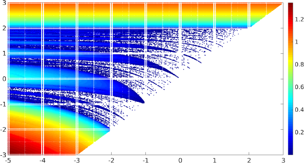
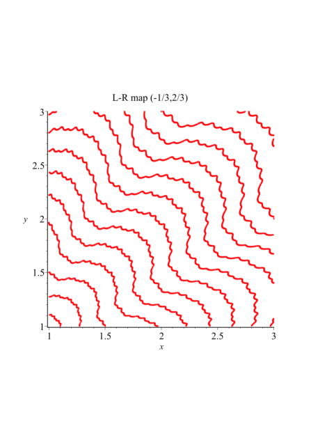
A family of algebraic curves defined by a dynamical condition, bounding the mode-locking regions [26, 24, 25, 9].

A central question regards the existence and properties of quasi-periodic orbits whose closure are topological circles, special cases of which occur for parameters of type i) and iii). General results are scarce. M. Herman’s work in the broader setting of the Froeschlé group [11, Theorem VIII.5.1] implies that any map $\mathrm{F}$ having an irrational rotation number $\theta=\theta(\mathrm{a},\mathrm{b})$ with bounded partial quotients in its continued fraction expansion is topologically conjugate to a rotation of the plane, and hence has invariant circles. This set of parameter values has zero two-dimensional Lebesgue measure. The results of [15] on curves of type iii) are complementary, as they regard one-dimensional sets of parameters (see below). Numerical experiments suggest ubiquity of parameter pairs for which all orbits are dense on non-smooth curves, as in figure 1, right.

The present work is devoted to the development of a theory of the curves of type iii), which we call the critical curves in parameter space. They are defined by the condition that an initial boundary ray (the positive or negative ordinate semi-axis in $\mathbb{R}^{2}$ ) be sent by the map $\mathrm{F}$ to the opposite boundary ray in a prescribed number of iterations. If the parameters $\mathrm{a},\mathrm{b}$ belong to critical curve, and if the rotation number of the corresponding circle map $\mathrm{f}$ is irrational, then the phase space of $\mathrm{F}$ foliates into piecewise smooth invariant curves, consisting of arcs of conic sections joined together [15, theorem 2.2]²²2The authors of [15] do not introduce explicitly the notion of critical curve..

We now summarise the contents and main results of this paper. In section 2 we provide some background on the symbolic dynamics of rotations and on the circle map $\mathrm{f}$ . We then give some preliminary results for the dynamics of $\mathrm{F}$ on a half-plane and its relation to the parameter. In the following section we introduce the main object of study, the critical curves, which correspond to the occurrence of Sturmian-type words in the symbolic dynamics (see [21, section 6]). Using the theory of continuants, we determine some general algebraic properties of these curves (propositions 5,7, section 3.1). We link the symbolic dynamics to the time-reversal symmetry of the map $\mathrm{F}$ (theorem 6), and show that critical curves have several disjoint branches, whose number is determined by the code. We establish that only one branch —indeed, only a part of it— is relevant to the dynamics of the map $\mathrm{F}$ (theorems 8 and 10), meaning that the code that defines the curve is the symbolic dynamics of a segment of an actual orbit of the map $\mathrm{F}$ , with initial condition of the appropriate boundary ray. Subsequently (section 3.2) we consider functions defined over critical curves, and derive formulae for the Poisson brackets of two curves (theorem 9), for later use.

In section 4 we consider intersections of critical curves, which lead to periodic orbits. We introduce the concept of intersection sequence, with which we classify the intersections of a curve with curves of lower degree generated by sub-words (theorem 11). We construct an associated geometrical object, called the polygonal of the curve, by means of which we formulate sufficient conditions for the transversality of these intersections (theorem 14). We also formulate conditions under which intersections delimit the portion of a curve which has dynamical significance.

In section 5 we consider the first generation of curves of type iii). These are obtained by concatenating the symbolic words of two curves of type i), and then allowing for repetitions of the concatenated word (theorem 18).

Identities of Chebyshev polynomials are collected in an appendix.

2. Background

2.1. Rotational words

For references for this section, see, e.g., [21, 1].

The rotational words are the symbolic dynamics of rotations with respect to a two-element partition of the circle. A rotational orbit has the form $x_{t}=\{\theta t+x_{0}\}$ for some $\theta,x_{0}\in[0,1)$ , where $\{\cdot\}$ denotes the fractional part. Without loss of generality, we choose the partition $I_{a}=[0,\rho)$ and $I_{b}=[\rho,1)$ , the subscript denoting the symbol associated to each interval. Thus a rotational word is determined by a triple $(\theta,\rho,x_{0})$ . Rotations are invertible, so all rotational words can be extended to the left; the extension is unique, apart from some notable special cases (see below).

If we denote by $\mathcal{L}_{n}$ the collection of all sub-words (or factors) of length $n$ in an infinite word $W$ , then the complexity function of $W$ is $\mathcal{K}(n)=|\mathcal{L}_{n}|$ . An infinite word is eventually periodic if and only if $\mathcal{K}(n)\leqslant n$ for some $n$ , so we require $\mathcal{K}(n)\geqslant n+1$ . For rotational words, $\mathcal{K}(n)$ is (eventually) an affine function of $n$ . The precise form of $\mathcal{K}$ depends on whether or not the boundary points $0$ and $\rho$ of the partition are on the same doubly-infinite orbit. If they are, we let $\ell$ be the transit time from one to the other; if they aren’t, we let $\ell=\infty$ . Then, irrespective of the initial condition $x_{0}$ , the rotational word has complexity [1, theorem 10]

(2)

\mathcal{K}(n)=\begin{cases}2n&n\leqslant\ell\\ n+\ell&n>\ell.\end{cases}

The case $\ell=1$ are the much studied Sturmian words [21, section 6]. If $1<\ell<\infty$ , we call the word quasi-Sturmian (of length $\ell$ ), and free if $\ell=\infty$ .

All irrational rotations are minimal (and indeed uniquely ergodic), and this implies that for fixed irrational $\theta$ and arbitrary $\rho$ , each factor of any rotational word occurs infinitely often and with bounded time between successive occurrences, hence with a well-defined frequency; the latter may be computed as the length of an interval [1]. The symbolic language [the sequence $(\mathcal{L}_{n})$ ] does not depend on the initial condition $x_{0}$ [21, p. 105], and for our purpose the parameter space for rotations will be the unit square $[0,1)^{2}$ . The parameters $\theta$ and $\rho$ will be referred to as the rotational parameters.

If the points $0$ and $\rho$ are on the same orbit, separated by $\ell$ iterations ( $\ell$ could be negative), then $\ell\theta\equiv\rho\,({\rm mod\ }1)$ , that is, the quasi-Sturmian configurations for a given $\ell$ correspond to a finite collection of segments in rotational parameter space.

2.2. The circle map

Let $\mathrm{f}:[0,1)\to[0,1)$ be the circle map associated to (1), namely

(3)

\mathrm{f}(e^{2\pi ix})=\frac{\mathrm{F}(e^{2\pi ix})}{\|\mathrm{F}(e^{2\pi ix})\|}\qquad e^{2\pi ix}\cong(\cos(2\pi x),\sin(2\pi x))\in\mathbb{R}^{2}.

This is an orientation-preserving homeomorphism whose derivative is continuous and of bounded variation [14, theorem 3.1]. Hence $\mathrm{f}$ has a well-defined rotation number $\theta=\theta(\mathrm{a},\mathrm{b})$ . The latter is a continuous function of the parameters, and its range is the interval $[0,1/2]$ [14, theorems 2.1 and 3.3]. From Denjoy theorem [12, p. 401], if $\theta$ is irrational then $\mathrm{f}$ is topologically conjugate to a rotation by $\theta$ , which in turn determines the symbolic language $\mathcal{L}$ , irrespective of the initial conditions.

We divide the domain of the circle map $\mathrm{f}$ into two intervals $I_{a}$ and $I_{b}$ , and associate to an orbit a symbolic word $W$ in the letters $a$ and $b$ , determined by the two branches of the map $\mathrm{F}$ in (1). We denote by $W_{n}$ the prefix of $W$ of length $n$ , and by $|W_{n}|_{w}$ the number of times the finite word (factor) $w$ appears in $W_{n}$ . The rotation number $\theta(\mathrm{a},\mathrm{b})$ and the density $\rho(\mathrm{a},\mathrm{b})$ are defined as follows:

(4)

\theta(\mathrm{a},\mathrm{b})=\lim_{n\to\infty}\frac{1}{n}|W_{n}(\mathrm{a},\mathrm{b})|_{ab},\qquad\rho(\mathrm{a},\mathrm{b})=\lim_{n\to\infty}\frac{1}{2n}\bigl{(}|W_{n}^{+}(\mathrm{a},\mathrm{b})|_{a}+|W_{n}^{-}(\mathrm{a},\mathrm{b})|_{a}\bigr{)},

where $W$ is arbitrary and $W^{\pm}$ is the word of the orbit with initial condition $(0,\pm 1)$ .

The above limits exist because they are frequencies of factors of rotational words. Since every appearance of the factor $ab$ corresponds to one loop around the origin, our definition of rotation number is equivalent to the standard one for circle homeomorphisms [12, chapter 11]; in particular, the rotation number is independent from the initial condition. This also holds for the density, as long as the rotation number is irrational, from minimality of irrational rotations (section 2.1). If the rotation number is rational, then the density may depend on the initial condition; in our definition (4) the union of the orbits corresponding to $W^{\pm}$ is invariant under time-reversal symmetry [because $\mathrm{F}(0,\mp 1)=(\pm 1,0)$ ]. This ensures that $\rho(\mathrm{a},\mathrm{a})=1/2$ for all real $\mathrm{a}$ , so that $\rho$ is continuous on the main diagonal in parameter space.

We consider the level sets of the rotation number:

(5)

\begin{array}[]{rcl}\Theta(x)&=&\{(\mathrm{a},\mathrm{b})\in\mathbb{R}^{2}\,|\,\theta(\mathrm{a},\mathrm{b})=x\}\end{array}\qquad 0\leqslant x\leqslant 1/2.

If $x=p/q$ is rational, then $\Theta(p/q)$ will be called a resonance.³³3We prefer this term to the customary terms tongue or sausage. A point $(\mathrm{a},\mathrm{b})$ of a resonance is a pinch-point if the set $\Theta(p/q)\setminus\{(\mathrm{a},\mathrm{b})\}$ is locally disconnected near $(\mathrm{a},\mathrm{b})$ . Note that the density $\rho$ is not necessarily continuous within a resonance, because the same rotation number may be associated to more than one code. For instance, the periodic codes $aabb$ and $abbb$ have the same rotation number 1/4, but distinct densities 1/2 and 1/4.

We now remove from the parameter space $\mathbb{R}^{2}$ of the circle map $\mathrm{f}$ the interior of the resonances $\Theta(0)$ and $\Theta(1/2)$ , given by

(6)

\Theta(1/2)=\{(\mathrm{a},\mathrm{b})\in\mathbb{R}^{2}\,|\,\mathrm{a}\mathrm{b}\leqslant 4,\mathrm{a},\mathrm{b}<0\},\qquad\Theta(0)=\{(\mathrm{a},\mathrm{b})\in\mathbb{R}^{2}\,|\,\max(\mathrm{a},\mathrm{b})\geqslant 2\}.

We obtain an infinite strip $\mathcal{A}$ , the region lying between the boundaries of $\Theta(0)$ and $\Theta(1/2)$ . (If we identify the points $(-\infty,\zeta)$ and $(\zeta,-\infty)$ , for $0\leqslant\zeta\leqslant 2$ , then $\mathcal{A}$ becomes a compact set —a topological annulus.)

A detailed investigation of parameter space outside resonances requires replacing original parameters $\mathrm{a},\mathrm{b}$ with the rotational parameters $\theta,\rho$ , which are suited for an arithmetical analysis of critical curves. This is the subject of a forthcoming investigation [23].

2.3. Basic dynamical properties

The area-preserving map $\mathrm{F}$ of (1) has a common form of a reversible map, i.e., a map conjugate to its inverse via an involution, specifically

(7)

\mathrm{F}^{-1}=\mathrm{R}\circ\mathrm{F}\circ\mathrm{R},\quad\mathrm{R}:(x,y)\mapsto(y,x).

Reversible maps are well-studied [17] and an equivalent definition is that they can be written as the composition of two involutions (e.g., $\mathrm{F}$ is the composition of $\mathrm{F}\circ\mathrm{R}$ and $\mathrm{R}$ ). An orbit of $\mathrm{F}$ is called symmetric if it is $\mathrm{R}$ -invariant and asymmetric otherwise, in which case it forms an asymmetric pair with its $\mathrm{R}$ -image. A symmetric orbit must contain one or two points from the symmetry lines

Fix(\mathrm{R})\cup Fix(\mathrm{F}\circ\mathrm{R}),

and is periodic if and only if it contains two points, where

(8)

Fix(\mathrm{R}):=\{(x,x):x\in\mathbb{R}\},\quad Fix(\mathrm{F}\circ\mathrm{R}):=\{(\frac{\mathrm{a}}{2}\,y,y):y>0\}\cup\{(\frac{\mathrm{b}}{2}\,y,y):y\leqslant 0\}.

As also realised in [14], a special role in the dynamics of $\mathrm{F}$ is played by the positive and negative ordinate semi-axes and we define:

(9)

L^{+}:=\{(0,y):y\geqslant 0\},\quad L^{-}:=\{(0,-y):y\geqslant 0\}.

We use the terminology $L^{+}$ -orbit of $\mathrm{F}$ for an orbit that contains $L^{+}$ and likewise an $L^{-}$ -orbit. An orbit that contains neither $L^{+}$ or $L^{-}$ will be called a non- $L^{\pm}$ orbit. Because of the scale invariance of $\mathrm{F}$ , it suffices to study the orbit of $(0,1)$ to find an $L^{+}$ orbit and the orbit of $(0,-1)$ to find an $L^{-}$ orbit. As a result, we will often identify $L^{+}$ , respectively $L^{-}$ , with $(0,1)$ , respectively $(0,-1)$ . More generally, the scale invariance of $\mathrm{F}$ allows us to talk interchangeably about an orbit of points in the plane and the associated orbit of rays where each point is embedded into its position vector from the origin.

An orbit of $\mathrm{F}$ is typically made from patching together orbit segments that occupy the domain of $\mathrm{M}_{a}=\left(\begin{smallmatrix}a&-1\\ 1&0\end{smallmatrix}\right)$ in the right half plane with orbit segments that switch to occupy the domain of $\mathrm{M}_{b}$ in the left half plane, before repeating this alternating behaviour. For reference, we denote these domains:

(10)

\mathrm{dom}(\mathrm{M}_{a}):=\bigl{\{}(x,y)\in\mathbb{R}^{2}\,:\,-\frac{\pi}{2}\leqslant\arctan_{2}(y,x)<\frac{\pi}{2}\bigr{\}},\quad\mathrm{dom}(\mathrm{M}_{b}):=\mathbb{R}^{2}\setminus\mathrm{dom}(\mathrm{M}_{a}).

In proposition 1 below, we study the dynamics within a single orbit segment in the right half plane (for ray counting in that result, note that $L^{-}\in\mathrm{dom}(\mathrm{M}_{a})$ but $L^{+}\in\mathrm{dom}(\mathrm{M}_{b}))$ .

Define the eigenvalues of $\mathrm{M}_{a}$ by

(11)

\lambda=\lambda_{\pm}=\frac{a}{2}\pm\sqrt{\biggl{(}\frac{a}{2}\biggr{)}^{2}-1},\quad\lambda_{+}\,\lambda_{-}=1.

When $|a|\leqslant 2$ , the elliptic case, we shall make use of the quantity

(12)

\zeta_{j}:=2\cos(\pi/j),\quad j=1,2,\ldots.

When $|a|>2$ , the hyperbolic case, the real eigenvectors associated to $\lambda_{\pm}$ are denoted $V_{\pm}$ and have slope $\lambda_{\mp}$ . From (69) in the appendix, the powers of $\mathrm{M}_{a}$ can be expressed in terms of polynomials ${U}_{n}(a)$ in $a$ of degree $n-1$ , with ${U}_{n}(a)={\bar{U}}_{n-1}(a/2)$ , where $\bar{U}_{n}$ is the $n$ th Chebyshev polynomial of the second kind. The polynomials $U_{n}$ satisfy

(13)

{U}_{-1}(a)=-1,\quad{U}_{0}(a)=0,\hskip 30.0pt{U}_{n+1}(a)=a\,{U}_{n}(a)-{U}_{n-1}(a),\quad n\geqslant 0.

From (69), the forward images of $(1,0)=\mathrm{M}_{a}(0,-1)$ by $\mathrm{M}_{a}^{j}$ for $j\geqslant 0$ , as long as they remain in $\mathrm{dom}(\mathrm{M}_{a})$ , are the rays

(14)

(U_{j+1}(a),U_{j}(a))\in\mathrm{dom}(\mathrm{M}_{a}),\quad\mbox{with slope}\quad m_{j}:=U_{j}(a)/U_{j+1}(a).

Likewise, by reversibility, the images of $\mathrm{R}\,(1,0)=(0,1)$ by $\mathrm{M}_{a}^{-j}$ are the rays

(15)

{\bf r}_{j}(a):=(U_{j}(a),U_{j+1}(a))\in\mathrm{dom}(\mathrm{M}_{a}),\quad\mbox{with slope }1/m_{j}.

The Mobius transformation that relates the slope $m$ of an initial ray in $\mathrm{dom}(\mathrm{M}_{a})$ to the slope $\mu_{a}(m)$ of its image is:

(16)

m\mapsto\mu_{a}(m)=\frac{1}{a-m},\quad m\in\mathbb{R}\cup\infty.

It inherits a reversing symmetry from $\mathrm{R}$ , given by

(17)

m\mapsto\frac{1}{m}.

We also note that order preservation of the induced circle map corresponding to $\mathrm{M}_{a}$ (or $\mathrm{M}_{b}$ ) means that if one ray is obtained from another by an anti-clockwise rotation then the same is true of their images. We use the anti-clockwise direction to order rays in the orbit segment from ‘first’ to ‘last’.

Proposition 1.

Consider the dynamics of $\mathrm{M}_{a}=\left(\begin{smallmatrix}a&-1\\ 1&0\end{smallmatrix}\right)$ in $\mathrm{dom}(\mathrm{M}_{a})$ of (10).

i)

For all $a>2$ , all rays between $L^{-}$ and the contracting eigenvector ray $V_{-}\,\cap\,\mathrm{dom}(\mathrm{M}_{a})$ with slope $\lambda_{+}>1$ converge onto the expanding eigenvector ray $V_{+}\,\cap\,\mathrm{dom}(\mathrm{M}_{a})$ with slope $\lambda_{-}<1$ —the points on these rays escape to infinity along this direction; the rays between $V_{-}\,\cap\,\mathrm{dom}(\mathrm{M}_{a})$ and $L^{+}$ eventually escape to $\mathrm{dom}(\mathrm{M}_{b})$ .
ii)

For any $\kappa\geqslant 2$ , we have $a=\zeta_{\kappa}$ of (12) if and only if there is a segment of a symmetric orbit that goes from $L^{-}$ to $L^{+}$ with $\kappa$ rays in $\mathrm{dom}(\mathrm{M}_{a})$ and ${\mathrm{M}_{a}}^{\kappa}=-Id$ .
iii)
When $a\in(\zeta_{\kappa-1},\zeta_{\kappa}),\kappa\geqslant 2$ , the possible orbit segments of $\mathrm{M}_{a}$ in $\mathrm{dom}(\mathrm{M}_{a})$ comprise a sequence of rays rotating anti-clockwise from the fourth quadrant into the first quadrant and eventually escaping to the left half-plane. The possibilities are:
1. a)
  
  a $L^{+}$ -orbit segment with $\kappa-1$ rays and first ray $(U_{\kappa-1}(a),U_{\kappa}(a))$ in the interior of the fourth quadrant;
2. b)
  
  a $L^{-}$ -orbit segment with $\kappa$ rays comprising $L^{-}=(0,-1)$ and $(1,0)$ and the $\mathrm{R}$ -image of the $L^{+}=(0,1)$ -orbit segment contained within the first quadrant.
3. c)
  
  a non- $L^{\pm}$ orbit segment with $\kappa-1$ rays if the first ray has slope $m$ with $U_{\kappa}(a)/U_{\kappa-1}(a)<m<0$ and $\kappa$ rays if the first ray has slope $m$ with $m<U_{\kappa}(a)/U_{\kappa-1}(a)<0$ .
iv)

The rays ${\bf r}_{j}(a)$ of (15) that delineate the sectors in item iii a) rotate anti-clockwise as $a$ increases.

Proof. Firstly, we make a general comment about orbit segments. Since $(0,-1)$ maps anti-clockwise to $(1,0)$ , independent of $a$ , any orbit segment in $\mathrm{dom}(\mathrm{M}_{a})$ not starting parallel to $(0,-1)$ must have a single ray, its first, in the interior of the fourth quadrant (which is the image under $\mathrm{M}_{b}$ of the last ray in the preceding orbit segment). This first ray with positive $x$ -coordinate has an image with positive $y$ -coordinate since $y^{\prime}=x$ in $\mathrm{F}$ . On the other hand, the image of $(0,1)$ by $\mathrm{M}_{a}^{-1}$ is $(1,a)$ and the last ray of any orbit segment of $\mathrm{M}_{a}$ that escapes to the left half plane must be the single ray of the orbit segment located in the wedge sector determined by $(1,a)$ and $L^{+}$ .

We prove i). When $a>2$ , $U_{j+1}(a)>U_{j}(a)\geqslant j$ for $j\geqslant 1$ so (14) and order preservation implies the forward orbit of $(1,0)$ , and hence that of any initial ray in the fourth quadrant, is confined thereafter to the first quadrant. Analysis of (16) confirms that the fixed point at $m_{-}=\lambda_{-}$ of (11) is attracting on $[-\infty,\lambda_{+})$ . The fixed point at $m_{+}=\lambda_{+}$ is repelling and the interval $(\lambda_{+},\infty)$ eventually is mapped to $m<0$ (which in this case corresponds to rays moving to the second quadrant). Of course, the fixed points $m_{\pm}=\lambda_{\pm}$ correspond to the eigenvectors of $\mathrm{M}_{a}$ .

We prove ii). For $\mathrm{M}_{a}^{-j}\,(0,1)=(U_{j}(a),U_{j+1}(a))$ , requiring $U_{j}(a)>0$ for $1\leqslant j<\kappa$ and $U_{\kappa}(a)=0$ produces $\kappa-1$ rays clockwise in the first quadrant, the last one parallel to $(1,0)$ . Since the pre-image of $(1,0)$ is $(0,-1)$ , we obtain $\kappa$ rays in total. For $\kappa=2$ , the condition on $a$ for this orbit is that $U_{2}(a)=a=0$ . For $\kappa>2$ , the condition $U_{j}(a)>0$ for $1\leqslant j<\kappa$ and $U_{\kappa}(a)=0$ finds the right-most root of $U_{\kappa}$ , namely $a=\zeta_{\kappa}$ . This follows from the well known roots of the Chebyshev polynomials $\bar{U}_{n}$ , as does the fact that $U_{\kappa-1}(\zeta_{\kappa})=1$ . Thus the $(\kappa-1)$ th ray is exactly $(1,0)$ , not just parallel to it. Substituting $U_{\kappa-1}(\zeta_{\kappa})=1$ , $U_{\kappa}(\zeta_{\kappa})=0$ and $U_{\kappa+1}(\zeta_{\kappa})=-1$ into (69) gives ${\mathrm{M}_{a}}^{\kappa}=-Id$ . Since $(1,0)=\mathrm{F}(0,-1)$ and $(0,1)$ are mapped to one another by $\mathrm{R}$ , the finite orbit segment from $L^{-}$ to $L^{+}$ is part of a symmetric orbit.

iii) For an $L^{+}$ -orbit segment of $\kappa-1$ rays, we require from (15) that $U_{j}(a)>0$ for $1\leqslant j<\kappa$ and $U_{\kappa}(a)<0$ , whence $a\in(\zeta_{\kappa-1},\zeta_{\kappa})$ , giving part a). These $\kappa-1$ rays, together with $L^{+}$ , delineate $\kappa$ sectors in $\mathrm{dom}(\mathrm{M}_{a})$ . Taking any ray internal to the first sector bounded by $L^{-}$ and $(U_{\kappa-1}(a),U_{\kappa}(a))$ and iterating gives an orbit segment of $\kappa$ rays in $\mathrm{dom}(\mathrm{M}_{a})$ , with one ray in each sector by order preservation. The first ray has slope $m:m<U_{\kappa}(a)/U_{\kappa-1}(a)<0$ . Taking any ray internal to the second sector starting at $(U_{\kappa-1}(a),U_{\kappa}(a))$ that is also in the fourth quadrant, with slope $m:U_{\kappa}(a)/U_{\kappa-1}(a)<m<0$ , gives an orbit segment of $\kappa-1$ rays. This proves part c). A $L^{-}$ orbit segment of $\kappa$ rays begins with $L^{-}$ and then a ray parallel to $(1,0)=\mathrm{R}\,(0,1)$ . From (14) and (15), the forward orbit of $(1,0)$ contained in the first quadrant is the $\mathrm{R}$ -image of the backwards orbit of $(0,1)$ contained in the first quadrant, which from b) comprises $\kappa-1$ rays including now $(0,1)$ itself.

We prove iv). The inverse of (16) is $m\mapsto{\mu_{a}}^{-1}(m)=a-\frac{1}{m}$ for $m\in\mathbb{R}\cup\infty$ , and it gives the slope $m(\mathrm{F}^{-1}z)=\mu_{a}^{-1}(m)$ in terms of the slope $m=m(z)$ of a ray $z\in\mathbb{R}^{2}$ . We apply this to the rays ${\bf r}_{j}(a)$ of (15) that delineate the sectors in proposition 1 iii) a). Defining $r_{j}(a):=m({\bf r}_{j}(a))$ , we have

r_{j+1}(a)=a-\frac{1}{r_{j}(a)}\implies r_{j+1}^{{}^{\prime}}=1+\frac{r_{j}^{{}^{\prime}}}{{r_{j}}^{2}},

where the prime denotes differentiation with respect to $a$ . Since $r_{0}=\infty,r^{{}^{\prime}}_{0}=0$ and $r_{1}=a,r_{1}^{{}^{\prime}}=1$ , then by induction, we see $r_{j}^{{}^{\prime}}\geqslant 1$ for $j\geqslant 1$ . Hence as $a$ increases, ${\bf r}_{j}(a)$ moves anti-clockwise.

There is the obvious version of the above for $\mathrm{M}_{b}$ .

This first dynamical analysis allows some preliminary bounds on rotation number and density in parameter space.

Proposition 2.

Let $\kappa\geqslant 2$ . If $\mathrm{a}\in(\zeta_{\kappa-1},\zeta_{\kappa}]$ , then the number of rays in each orbit segment in $\mathrm{dom}(\mathrm{M}_{a})$ is $\kappa-1$ or $\kappa$ . If $\mathrm{b}\in(\zeta_{\ell-1},\zeta_{\ell}]$ , $\ell\geqslant 2$ , the analogous result holds in $\mathrm{dom}(\mathrm{M}_{b})$ and in addition:

(i)\enspace\theta(\mathrm{a},\mathrm{b})\in\bigl{[}\frac{1}{\kappa+\ell},\frac{1}{\kappa+\ell-2}\bigr{]};\qquad(ii)\enspace\rho(\mathrm{a},\mathrm{b})\in\bigl{[}\frac{\kappa-1}{\kappa+\ell-1},\frac{\kappa}{\kappa+\ell-1}\bigr{]}.

Proof. The statement on the number of rays versus parameter value follows directly from the list of possibilities in proposition 1. If we use $N_{a}^{i}=N_{a}^{i}(\mathrm{a},\mathrm{b})$ , $i\in\mathbb{Z}$ , to label the bi-infinite sequence of the number of rays in $\mathrm{dom}(M_{a})$ indexed by revolution $i$ , and similarly for $N_{b}^{i}$ , then

$\displaystyle\theta(\mathrm{a},\mathrm{b})$	$\displaystyle=$	$\displaystyle\lim_{k\to\infty}\frac{2k+1}{\sum_{i=-k}^{i=k}N_{a}^{i}+N_{b}^{i}},$
$\displaystyle\rho(\mathrm{a},\mathrm{b})$	$\displaystyle=$	$\displaystyle\lim_{k\to\infty}\frac{\sum_{i=-k}^{i=k}N_{a}^{i}}{\sum_{i=-k}^{i=k}N_{a}^{i}+N_{b}^{i}}$
	$\displaystyle=$	$\displaystyle\lim_{k\to\infty}\bigl{(}1+\frac{\sum_{i=-k}^{i=k}N_{b}^{i}}{\sum_{i=-k}^{i=k}N_{a}^{i}}\bigr{)}^{-1}.$

Using the bounds $(2k+1)\,(\kappa-1)\leqslant\sum_{i=-k}^{i=k}N_{a}^{i}\leqslant(2k+1)\,\kappa$ etc., gives the results. Also we observe

\rho(\mathrm{a},\mathrm{b})=K(\mathrm{a})\,\theta(\mathrm{a},\mathrm{b}),

where $K(\mathrm{a}):=\lim_{k\to\infty}\frac{\sum_{i=-k}^{i=k}N_{a}^{i}}{2k+1}$ and $\kappa-1\leqslant K\leqslant\kappa$ .

Figure 2. Partition of the first quadrant

[0,2]^{2}

of the parameter space

\mathcal{A}

into rotational domains, determined by the critical curves of proposition 3. The boundary of

\Theta(0)

is represented in blue, and positive and negative critical words in red. The rational pairs near highlighted points represent the value of rotational parameters at those points.

3. Critical curves

A boundary parameter is a pair $(\mathrm{a},\mathrm{b})\in\mathcal{A}$ for which there is an $\mathrm{F}$ -orbit (a boundary orbit) that contains two (not necessarily distinct) boundary rays, namely the positive and negative ordinate semi-axes $L^{+}$ and $L^{-}$ of (9). Such a dynamical condition is accompanied by a finite boundary word $w$ , which encodes the itinerary between two boundary rays; this part of the boundary orbit will be called a boundary segment. Because the two components of the map $\mathrm{F}$ coincide on boundary rays, changing any letter that corresponds to a boundary ray has no effect on the orbit. (This always applies to the first letter of a boundary word.) The resulting ambiguity defines an equivalence relation on words, whereby we write $w\sim w^{\prime}$ to indicate that $w^{\prime}$ is obtained from $w$ by any change in the symbols allocated to a boundary ray. A boundary word which is equivalent, but not equal, to the symbolic dynamics of the map $\mathrm{F}$ is said to be improper. These words appear at the intersections of curves (section 4).

The rank $\iota$ of a boundary word $w$ is given by $\iota=1+|w|_{ab}+|w|_{ba}$ [cf. definition (4)]. If $w$ encodes the symbolic dynamics of $\mathrm{F}$ , then $\iota$ is the number of half-loops that occur in the transit between the initial and final boundary rays. A boundary word begins and ends with the same symbol in the odd-rank cases ( $L^{+}\mapsto L^{-}$ or $L^{-}\mapsto L^{+}$ ) and with distinct symbols in the even-rank case ( $L^{+}\mapsto L^{+}$ or $L^{-}\mapsto L^{-}$ ). The sign of a boundary word is positive if the word begins with the symbol $a$ (the orbit starts from $L^{-}$ ), and negative otherwise.

If the rank of $w$ is even, then the critical curve is the parametric locus of a periodic orbit having (at least) one point on the partition boundary. These are the periodic $\beta$ -orbits in [9, section 3.1], in which case the length and rank of the boundary word are, respectively, the denominator and twice the numerator of the rotation number. If an even rank curve supports both positive and negative boundary segments, then we call it an axis (of a resonance).

If the rank of a word $w$ is odd, then the set of parameters for which $w$ is a boundary word will be called a critical curve, examples of which are given in [15, examples 4.1–3] (see proposition 3 below). The associated boundary orbit of $\mathrm{F}$ will be called a critical orbit in this case.

We see that the orbits of proposition 1 ii) are critical orbits of rank 1 with critical curve $\mathrm{a}=\zeta_{\kappa}$ and boundary word $a^{\kappa}$ and this is true independently of the value of $\mathrm{b}$ and the dynamics in $\mathrm{dom}(\mathrm{M}_{b})$ . This is also the family i) mentioned in the introduction, which will be used in section 5. The following result extends example 3.2 in [14] (cf. also propositions 1 and 2 of the previous section):

Proposition 3.

For $\kappa=2,3,\ldots$ , the set

(18)

\mathbf{C}_{a^{\kappa}}:=\{(\zeta_{\kappa},\mathrm{b})\,:\,\mathrm{b}\in\mathbb{R}\},

with $\zeta_{\kappa}$ of (12) has rotational parameters

(19)

\rho(\zeta_{\kappa},\mathrm{b})=\kappa\theta(\zeta_{\kappa},\mathrm{b}),\hskip 40.0pt\theta(\zeta_{\kappa},\mathrm{b})=\begin{cases}0&\mathrm{b}>2\\ \vskip 3.0pt\cr\displaystyle\frac{\arccos(\mathrm{b}/2)}{\kappa\arccos(\mathrm{b}/2)+\pi}&|\mathrm{b}|\leqslant 2\\ \vskip 3.0pt\cr\displaystyle\frac{1}{\kappa+1}&\mathrm{b}<-2.\end{cases}

Exchanging $\mathrm{a}$ and $\mathrm{b}$ yields the twin sets $\mathbf{C}_{b^{\ell}}:=\{(\mathrm{a},\zeta_{\ell})\,:\,\mathrm{a}\in\mathbb{R}\}$ , with the corresponding formula for the rotation number and $\rho(\mathrm{a},\zeta_{\ell})=1-\rho(\zeta_{\ell},\mathrm{a})$ .

Proof. The rotation number in (19) for $|\mathrm{b}|\leqslant 2$ follows from example 3.2 and theorem 2.1 in [14]. The value of $\theta$ for $\mathrm{b}>2$ follows from (the $\mathrm{b}$ -part of) proposition 1 and the proof of proposition 2. If $\mathrm{b}\leqslant-2$ , then by (19) we have $\theta(\zeta_{\kappa},-2)={1}/{(\kappa+1)}$ , and by [14, theorem 2.1], $\theta(\mathrm{a},\mathrm{b})$ is nonincreasing in $\mathrm{b}$ , so that $\theta(\zeta_{\kappa},\mathrm{b})\geqslant 1/(\kappa+1)$ . However, (ii) of the same theorem implies $0\leqslant\theta(\zeta_{\kappa},\mathrm{b})\leqslant 1/(\kappa+1)$ for any $\mathrm{b}$ , and thus we have $\theta(\zeta_{\kappa},\mathrm{b})=1/(\kappa+1)$ for $\mathrm{b}\leqslant-2$ .

The density in (19) follows from $K(\mathrm{a})$ defined in the proof of proposition 2, noting from proposition 1 ii) that for $\mathrm{a}=\zeta_{\kappa}$ , we have $N_{\mathrm{a}}^{i}=\kappa$ for all $i$ , whence $K(\zeta_{\kappa})=\kappa$ . Exchanging $\mathrm{a}$ and $\mathrm{b}$ yields the same analysis; the obvious modification for the density results from the congruence $\rho\equiv\kappa\theta\,({\rm mod\ }1)$ with negative $\kappa$ .

Note that in the interval $|\mathrm{b}|\leqslant 2$ ( $|\mathrm{a}|\leqslant 2$ ) these components do not intersect the interior of any resonance, by virtue of the fact that the rotation number is nowhere constant. The points $(\zeta_{\kappa},\pm 2)$ of $\mathbf{C}_{a^{\kappa}}$ lie on the boundary of the resonances with rotation number $0$ and $1/(\kappa+1)$ .

The critical curves are our main object of study, and the closure of the set of boundary parameters which belong to some critical curve will be called the critical set $\Xi\subset\mathcal{A}$ . The simplest components of the critical set are those described in proposition 3. Indeed, for $\kappa\geqslant 2$ , the positive word $a^{\kappa}=\underbrace{a\cdots a}_{\kappa}$ is critical of rank one, with components $\mathbf{C}_{a^{\kappa}}$ . Likewise, $b^{\ell}$ is negative of rank one, with component $\mathbf{C}_{b^{\ell}}$ .

For later use, we collect the following which are known or easily verified:

Lemma 4.

For the map $\mathrm{F}=\mathrm{F}_{ab}$ of (1) and its reversing symmetry $\mathrm{R}$ of (7), we have:

i)

From reversibility, the $\mathrm{R}$ -image of the forward (backward) orbit of $(0,y)$ is the backward (forward) orbit of $\mathrm{R}\,(0,y)=(y,0)=\mathrm{F}(0,-y)$ , i.e.,

$\mathrm{F}^{-k+1}\,(0,-y)=\mathrm{R}\,\mathrm{F}^{k}\,(0,y),\quad k\in\mathbb{Z},\;y\in\mathbb{R}^{+}.$
ii)

A critical orbit of odd rank exists if and only if $(0,1)$ and $\mathrm{R}\,(0,1)=(1,0)=\mathrm{F}(0,-1)$ are in the same orbit. Since the point $(0,1)$ and its image under $R$ are in the same orbit, the critical orbit is symmetric.
iii)

With $T:(x,y)\mapsto(-x,-y)$ , we have

$\mathrm{F}_{ab}=T\circ\mathrm{F}_{ba}\circ T^{-1}.$

In particular, it suffices to study critical orbits where $(0,-1)$ goes to $(0,1)$ in forward time as those from $(0,1)$ to $(0,-1)$ for $F_{ab}$ map to the former for $F_{ba}$ .
iv)

There can be no critical orbit (of rank $>1)$ from $(0,-1)$ to $(0,1)$ if $a>2$ ( $b>2$ ).
v)

We have $\mathrm{F}(0,\pm 1)=(\mp 1,0)$ together with $\mathrm{F}(1,0)=(a,1),\;\mathrm{F}(-1,0)=(-b,-1)$ and $\mathrm{F}^{-1}(0,1)=(1,a),\mathrm{F}^{-1}(0,-1)=(-1,-b)$ . Additionally:
(a) each orbit segment in $\mathrm{dom}(\mathrm{M}_{a})$ $(\mathrm{dom}(\mathrm{M}_{b}))$ only has at most one point in the interior of the fourth (second) quadrant, with its image in the first or second (third or fourth) quadrant;
(b) if $a,b\in(-2,2)$ , and if an orbit segment has a point $P$ in the interior of the first (third) quadrant, then some image $\mathrm{F}^{j}\,P$ with $j\geq 1$ is in the second (fourth) quadrant and some pre-image $\mathrm{F}^{-k}\,P$ with $k\geq 1$ is in the fourth (second) quadrant.

Proof. Property i) is a standard result for reversible maps [17]. Property ii) is from [14, theorem 3.4]. Property iii) is from [14, equation (2.4)]. Property iv) follows from Proposition 1 i) and its corresponding version for $\mathrm{M}_{b}$ . Property v) follows from $\mathrm{F}$ being order preserving and $\mathrm{F}:(x,y)\mapsto(x^{\prime},y^{\prime})$ having $y^{\prime}=x$ and $\mathrm{F}^{-1}:(x^{\prime},y^{\prime})\mapsto(x,y)$ having $x=y^{\prime}$ .

3.1. Algebraic properties

Requiring that an orbit contain two boundary rays leads to algebraic curves over $\mathbb{Q}$ . We introduce the necessary formalism, and establish some properties of these curves.

Let

(20)

\mathrm{M}_{x}=\left(\begin{matrix}x&-1\\ 1&0\end{matrix}\right)

where $x$ is an indeterminate and consider the finite word

w=w_{0}w_{1}\cdots w_{t-1},

where we regard, for now, each letter of the word $w$ as an indeterminate (in the case of $\mathrm{F}$ , we will later specialise to $w_{i}\in\{a,b\}$ ). We form a product of matrices of type (20) as follows:

(21)

\mathrm{M}_{\varnothing}=\mathrm{Id},\qquad\mathrm{M}_{[w]}=\mathrm{M}_{w_{t-1}}\mathrm{M}_{w_{t-2}}\cdots\mathrm{M}_{w_{0}},

where $\varnothing$ denotes the empty word.

The entries of $\mathrm{M}_{[w]}$ are polynomials in the indeterminates $w_{0},w_{1}\cdots,w_{t-1}$ . Define the recursive sequence of polynomials $Q_{t}=Q_{t}(w_{1},\ldots,w_{t-1})\in\mathbb{Z}[w_{0},w_{1},\ldots,w_{t-1}]$ by the three-term recurrence:

(22)

\begin{array}[]{llll}Q_{-1}=-1&\quad Q_{0}=0&\hskip 30.0ptQ_{t+1}=w_{t}Q_{t}-Q_{t-1}&\quad t\geqslant 0.\end{array}

Hence

$\displaystyle Q_{1}$	$\displaystyle=$	$\displaystyle 1,$
$\displaystyle Q_{2}(w_{1})$	$\displaystyle=$	$\displaystyle w_{1},$
$\displaystyle Q_{3}(w_{1},w_{2})$	$\displaystyle=$	$\displaystyle w_{1}w_{2}-1,$
$\displaystyle Q_{4}(w_{1},w_{2},w_{3})$	$\displaystyle=$	$\displaystyle w_{1}w_{2}w_{3}-w_{1}-w_{3},$
$\displaystyle Q_{5}(w_{1},w_{2},w_{3},w_{4})$	$\displaystyle=$	$\displaystyle w_{1}w_{2}w_{3}w_{4}-w_{1}w_{4}-w_{3}w_{4}-w_{1}w_{2}+1.$

Alternatively, we can use the tridiagonal determinant representation:

(23)

Q_{t}(w_{1},\ldots,w_{t-1}):=\begin{vmatrix}w_{1}&1&0&\cdots&0\\ 1&w_{2}&1&&\vdots\\ 0&\ddots&\ddots&\ddots&0\\ \vdots&&1&w_{t-2}&1\\ 0&\cdots&0&1&w_{t-1}\\ \end{vmatrix},\quad t\geq 2,

with the recurrence relation (22) following by expanding the determinant along the last row. Note we can also run the recurrence (22) backwards using indeterminates $w_{-i}$ to find:

(24)

Q_{-t}=-Q_{t}(w_{i}\mapsto w_{-i})\qquad t\geqslant 0.

With $Q_{t}$ defined, it follows by induction:

(25)

\mathrm{M}_{[w_{1}\cdots w_{t-1}]}=\begin{pmatrix}Q_{t}(w_{1},\ldots,w_{t-1})&-Q_{t-1}(w_{2},\ldots,w_{t-1})\\ Q_{t-1}(w_{1},\ldots,w_{t-2})&-Q_{t-2}(w_{2},\ldots,w_{t-2})\end{pmatrix},

and

(26)

\mathrm{M}_{[w_{0}\cdots w_{t-1}]}=\mathrm{M}_{[w_{1}\cdots w_{t-1}]}\mathrm{M}_{[w_{0}]}=\begin{pmatrix}w_{0}Q_{t}-Q_{t-1}&-Q_{t}\\ w_{0}Q_{t-1}-Q_{t-2}&-Q_{t-1}\end{pmatrix}\qquad t\geqslant 1.

The above results follow from the theory of continuants (or continuant polynomials), a name given to the tridiagonal determinant (23). Continuants and their properties were studied by Euler [10, Section 6.7] in connection with generalised continued fractions involving arbitrary real (or complex) numbers instead of integers, see proposition 5 i) below. The associated three-term recurrence for Euler’s original continuant is for the polynomial sequence $q_{t}$ satisfying $q_{-1}=-1$ , $q_{0}=0$ and $q_{t+1}=w_{t}q_{t}+q_{t-1}$ . The polynomial $Q_{t}$ of (22) belongs to a class of generalisations of the classic continuant, variously called signed continuant polynomials or generalised Chebyshev polynomials, which have arisen in the study of cluster algebras and frieze patterns [19, 2]. The relationship between $Q_{t}$ and $q_{t}$ is $Q_{t}(w_{1},\ldots,w_{t-1})=(-i)^{t-1}\,q_{t}(i\,w_{1},\ldots,i\,w_{t-1})$ with $i=\sqrt{-1}$ .

It follows from Euler that $Q_{t}$ can be generated as the sum of the product $w_{1}w_{2}\ldots w_{t-1}$ , its leading term, together with all possible ways of writing the leading term again but striking out adjacent product pairs $w_{i}w_{i+1}$ and replacing such a pair with $-1$ (e.g., the four non-leading terms of $Q_{5}$ above are obtained by striking out, respectively, $w_{2}w_{3}$ , $w_{1}w_{2}$ , $w_{3}w_{4}$ and the two pairs $w_{1}w_{2}$ and $w_{3}w_{4}$ ). Note that from (22) and (13),

(27)

Q_{n+1}(x,x,\ldots x)={U}_{n+1}(x)=\bar{U}_{n}(x/2),

where $\bar{U}_{n}$ are the Chebyshev polynomials of the second kind —see the Appendix.

We shall need the following properties of continuants, found in references [10, Chapter 6.7][19, Section 5.1], [2, Section 2.2]: [10, 19, 2],

Proposition 5 (Continuant Polynomials).

For all $t>1$ , indeterminates $w_{1},\ldots,w_{t-1}\in\mathbb{R}$ and integers $k,l\geqslant-1$ , we have

i)

$\displaystyle\frac{Q_{t}(w_{1},\ldots,w_{t-1})}{Q_{t-1}(w_{2},\ldots,w_{t-1})}=\,w_{1}-\frac{1}{\displaystyle\,w_{2}-\frac{1}{\displaystyle\,\ddots-\frac{1}{w_{t-1}}}}$
ii)

$\displaystyle Q_{t}(w_{1},\ldots,w_{t-2},w_{t-1})=Q_{t}(w_{t-1},w_{t-2},\ldots,w_{1})$
iii)

$\displaystyle Q_{k+l+1}(w_{1},\ldots,w_{k+l})=\\ Q_{k+1}(w_{1},\ldots,w_{k})\,Q_{l+1}(w_{k+1},\ldots,w_{k+l})-Q_{k}(w_{1},\ldots,w_{k-1})\,Q_{l}(w_{k+2},\ldots,w_{k+l}).$

We now specialise to the case of odd rank, for which the structure of words and curves is constrained by the reversibility of the map. The reduced word $\underline{w}$ of $w$ is defined as $\underline{w}=w_{1}\cdots w_{n-1}$ (again reversibility dictates considering to drop the first letter $w_{0}$ – see below). We say that $\underline{w}$ is a palindrome if

w_{i}=w_{n-i}\qquad i=1,\ldots,n-1.

For $\mathrm{F}$ , the structure of a (palindromic) reduced boundary word of odd rank can also be encoded by the (palindromic) integer exponent sequence $(i_{k})$ of odd length $2m-1$ , using $i_{k}\in\mathbb{Z}^{+}$ , $1\leqslant k\leqslant m$ , that we call its block sequence, e.g.,

(28)

\underline{w}=a^{i_{1}}\,b^{i_{2}}\,a^{i_{3}}\,\ldots b^{i_{m-1}}a^{i_{m}}\,b^{i_{m-1}}\,\ldots a^{i_{3}}\,b^{i_{2}}\,a^{i_{1}}.

In this form, the rank is now obvious, being $2m-1$ , whereas

(29)

i_{m}+2\,\sum_{k=1}^{m-1}i_{k}=n-1.

We take the convention that $i_{k}$ , $k$ odd, counts powers of $a$ if the associated word is positive as in (28) (recall this means the word begins with $a$ ) and powers of $b$ if the word is negative. We see for a positive palindromic word that the middle block comprises powers of $a$ when $m$ is odd and powers of $b$ when $m$ is even. We recall from proposition 2 that necessarily:

(30)

\mathrm{a}\in(\zeta_{\kappa-1},\zeta_{\kappa})\implies i_{k}\in\{\kappa-1,\kappa\},\quad\mathrm{b}\in(\zeta_{\ell-1},\zeta_{\ell})\implies i_{k}\in\{\ell-1,\ell\}.

The significance of palindromic words to boundary curves of the map $\mathrm{F}$ is established by the following result (it suffices to prove the case of a positive word noting ii) and iii) of lemma 4).

Theorem 6.

Consider a non-periodic critical orbit of $\mathrm{F}$ that contains $(0,-1)$ and $(0,1)$ and the associated positive boundary word $w$ of length $n$ that encodes the itinerary between them. We have:

i)

The reduced boundary word of rank $2m-1$ is a palindrome (28) of $2m-1$ blocks (equivalently its block sequence is a palindromic $(2m-1)$ -tuple of positive integers)
ii)

The integer $n$ is odd and $i_{m}$ is even if and only if the boundary segment intersects $Fix(\mathrm{R})$ once in $\mathrm{dom}(\mathrm{M}_{a})$ $(\mathrm{dom}(\mathrm{M}_{b}))$ , whence $m$ is odd (even).
iii)

The integer $n$ is even and $i_{m}$ is odd if and only if the boundary segment intersects $Fix(\mathrm{F}\circ\mathrm{R})$ once. The intersection is in $\mathrm{dom}(\mathrm{M}_{a})$ $(\mathrm{dom}(\mathrm{M}_{b}))$ if $i_{m}=1$ and $m$ is even (odd) or if $i_{m}>1$ and $m$ is odd (even).

Proof. i). From reversibility, for arbitrary $z\in\mathbb{R}^{2}$ , we have $z^{\prime}=\mathrm{F}(z)\iff\mathrm{R}z=\mathrm{F}(\mathrm{R}z^{\prime})$ . We claim the symbol sequence of the $\mathrm{F}$ -orbit leaving the point $z\not=(0,\pm 1)$ , developing to the right, is the same as the symbol sequence for the $\mathrm{F}$ -orbit arriving to $\mathrm{R}z$ , developing to the left. To see this, note the first symbol for the former is determined by $z$ and the first symbol for the latter is determined by $\mathrm{R}z^{\prime}$ and we claim that these symbols are the same. From proposition 4 v), we have that if $z$ is in the first or fourth quadrant, hence encoded with symbol $a$ for its forward image, then $z^{\prime}$ is in the first or second quadrant, whence $\mathrm{R}z^{\prime}$ is in the first or fourth quadrant, and $\mathrm{R}z^{\prime}$ is encoded similarly to $z$ . A similar result is true for $z$ in the second or third quadrant and the symbol $b$ . The argument is then iterated, next with $z^{\prime}$ and $\mathrm{R}\mathrm{F}(z^{\prime})$ . If we take a critical orbit with $z=(1,0)=\mathrm{F}(0,-1)$ , we see the finite orbit connecting $z$ and $\mathrm{R}z=(0,1)$ must have a palindromic symbol sequence, i.e., the reduced word is a palindrome as in (28).

We prove ii). We know a critical orbit is symmetric from lemma 4. In general [17], for any $G$ that acts as a reversor of a reversible map $L$ , so $L^{-1}=G^{-1}\circ L\circ G$ , an orbit is $G$ -invariant if and only if $G\,z=L^{k_{z}}z$ with $k_{z}\in\mathbb{Z}$ for each point $z\in\mathbb{R}^{2}$ of the orbit. The latter is true if and only if it is true for one point. Then either:
(a) $G\,L^{j_{z}}\,z=L^{j_{z}}\,z$ if $k_{z}=2j_{z}$ , i.e., $L^{j_{z}}\,z$ is fixed by $G$ ; or
(b) $LG\,L^{j_{z}+1}z=L^{j_{z}+1}z$ if $k_{z}=2\,j_{z}+1$ , i.e., $L^{j_{z}+1}z$ is fixed by $LG$ . If a symmetric orbit is not periodic, it contains one point fixed by $G$ or one point fixed by $LG$ .

We are interested in $L=\mathrm{F}$ and $G=\mathrm{R}$ and we can take the point $z=(1,0)$ and $k_{z}=n-1$ . If $n$ is odd so $k_{z}$ is even, we have case (a). Hence the forward orbit of the midway point $\mathrm{F}^{k_{z}/2}\,(1,0)\in Fix(\mathrm{R})$ is the reflection by $\mathrm{R}$ of its backwards orbit and the slope of the rays in the forward and backwards orbit are reciprocals of each other from (17). The involution $\mathrm{R}$ preserves the first and third quadrants and interchanges the second and the fourth. If $m>1$ is even (odd), the middle block in (28) is built from the letter $b$ (the letter $a$ ) and the number of points $i_{m}$ of this orbit segment in $\mathrm{dom}(M_{b})$ ( $\mathrm{dom}(M_{a})$ ) must be even. It comprises $\mathrm{F}^{k_{z}/2}\,(1,0)$ on the line $y=x$ and pairs of its forward and backward iterates in the interior of the third (first) quadrant, plus the necessary additional point in the second (fourth) quadrant guaranteed from lemma 4. If $m=1$ , we have only a single letter in the word and then $i_{m}$ in the reduced word is even (and the power is odd in the full word, cf. proposition 1). Hence $i_{m}$ is even as claimed, which can also be seen from (29).

We prove iii). Now consider the case (b) above, i.e., $n$ is even so $k_{z}$ is odd and $q=\mathrm{F}^{j_{z}+1}\,(1,0)\in Fix(\mathrm{F}\mathrm{R})$ . For $y>0$ , the involution $\mathrm{F}\mathrm{R}:x^{\prime}=-x+ay,y^{\prime}=y$ is a horizontal reflection about the point $\frac{a}{2}\,y$ ; for $y<0$ , it is a horizontal reflection about the point $\frac{b}{2}\,y$ . We have $\mathrm{F}^{j}\,q=\mathrm{F}^{j}\,(\mathrm{F}\mathrm{R}\,q)=(\mathrm{F}\mathrm{R})(\mathrm{F}^{-j}\,q)$ , so the forward and backward iterates of $q$ under $\mathrm{F}$ at corresponding times in the upper half-plane and in the lower half-plane must be pairs under these reflections. As an example, suppose $q\in\mathrm{dom}(\mathrm{M}_{a})$ in the first quadrant. This means the single ray in the second quadrant when $\mathrm{F}^{r}q$ first enters it (cf. lemma 4) must force the iterates of $q$ in the first quadrant to have $r-1$ rays to the left of $x=\frac{a}{2}\,y$ in forwards time, $r\geqslant 1$ , and $r$ rays to the right in backward time. Counting $q$ itself and the single ray $\mathrm{F}^{-(r+1)}\,q$ in the fourth quadrant gives $2r+1$ for the number $i_{m}$ of the letter $a$ in the middle block, whence $i_{m}$ is odd. Similar reasoning applies for the other possibilities.

This result leads us to study continuant polynomials for palindromic words (interestingly, palindromic continuants were used in Smith’s 1855 proof of the Fermat two-square theorem [6]). For generality, we again let $w=w_{0}\cdots w_{n-1}$ be a word in $n$ letters (not just two letters $a$ and $b$ ). Let

(31)

\mathbf{k}=\lfloor n/2\rfloor.

and build the particular polynomials in $\mathbb{Z}[w_{0},\ldots,w_{n-1}]$ from (22):

(32)

C_{w}:=\begin{cases}Q_{\mathbf{k}+1}-Q_{\mathbf{k}}&\mbox{$n$ odd}\\ Q_{\mathbf{k}+1}-Q_{\mathbf{k}-1}&\mbox{$n$ even}\end{cases}\hskip 35.0pt\tilde{C}_{w}:=\begin{cases}Q_{\mathbf{k}+1}+Q_{\mathbf{k}}&\mbox{$n$ odd}\\ Q_{\mathbf{k}}&\mbox{$n$ even}.\end{cases}

For completeness, if the rank of $w$ is even, we let $C_{w}=Q_{n}$ and $\tilde{C}_{w}=1$ .

The following result collects some algebraic properties of the $Q_{t}$ polynomials for palindromic words in any alphabet.

Proposition 7.

If $w_{1}\cdots w_{n-1}$ is a palindrome (in any alphabet), then the following holds for the polynomials $Q_{t}$ of (22) with $t=0,\ldots,n$ (noting also (24) for (ii)):

(33)		$\displaystyle i)$		$\displaystyle Q_{n}=C_{w}\tilde{C}_{w}$
(34)		$\displaystyle ii)$		$\displaystyle Q_{n-t}-Q_{t}=C_{w}\times\begin{cases}Q_{t-\mathbf{k}+1}(w_{\mathbf{k}}=-1,w_{\mathbf{k}+1},\ldots,w_{t-1})&\mbox{$n$ odd}\\ -Q_{t-\mathbf{k}}(w_{\mathbf{k}+1},\ldots,w_{t-1})&\mbox{$n$ even}.\end{cases}$

Proof. i) From proposition 5 ii) and iii) with $l=t-1$ , $k=n-t$ and the palindromic word, we have for $t=1,\ldots,n-1$ :

(35)

.\begin{split}Q_{n}(w_{1},\ldots,w_{n-1})&=\\ Q_{n-t+1}(w_{1},\ldots,w_{n-t})\,Q_{t}(w_{1},\ldots,w_{t-1})&-Q_{n-t}(w_{1},\ldots,w_{n-t-1})\,Q_{t-1}(w_{1},\ldots,w_{t-2}).\end{split}

For odd $n=2\mathbf{k}+1$ , we take $t=\mathbf{k}+1$ , to obtain $Q_{n}=Q_{\mathbf{k}+1}^{2}-Q_{\mathbf{k}}^{2}=C_{w}\tilde{C}_{w}$ . For even $n=2\mathbf{k}$ , we take $t=\mathbf{k}=n-t$ , giving $Q_{n}=Q_{\mathbf{k}+1}Q_{\mathbf{k}}-Q_{\mathbf{k}}Q_{\mathbf{k}-1}=C_{w}\tilde{C}_{w}$ .

ii) We prove the result by induction, in the first instance for $t\geqslant\mathbf{k}$ . Consider the polynomial $A_{t}=Q_{n-t}-Q_{t}$ . If $n=2\mathbf{k}+1$ , from (32) we find:

A_{\mathbf{k}}=Q_{\mathbf{k}+1}-Q_{\mathbf{k}}=C_{w}=C_{w}\,Q_{1}\qquad A_{\mathbf{k}+1}=Q_{\mathbf{k}}-Q_{\mathbf{k}+1}=-C_{w}=C_{w}\,Q_{2}(w_{\mathbf{k}}=-1).

If $n=2\mathbf{k}$ , then

A_{\mathbf{k}}=Q_{\mathbf{k}}-Q_{\mathbf{k}}=0=C_{w}\,Q_{0}\qquad A_{\mathbf{k}+1}=Q_{\mathbf{k}-1}-Q_{\mathbf{k}+1}=-C_{w}=C_{w}\,(-Q_{1}).

The above data serves as the base case for induction. Assume that (34) holds for all $i$ in the range $\mathbf{k}\leqslant i\leqslant t$ , for some $t\geqslant\mathbf{k}+1$ . Then

	$\displaystyle A_{t+1}$	$\displaystyle=$	$\displaystyle Q_{n-(t+1)}-Q_{t+1}=w_{n-t}Q_{n-t}-Q_{n-(t-1)}-w_{t}Q_{t}+Q_{t-1}$
		$\displaystyle=$	$\displaystyle w_{t}\,(Q_{n-t}-Q_{t})-(Q_{n-(t-1)}-Q_{t-1})=C_{w}\,(w_{t}S_{t}-S_{t-1})=C_{w}\,S_{t+1},$

where $S_{t}$ denotes the particular solutions in (34) for the respective cases of $n$ even and $n$ odd, which obviously satisfy $S_{t+1}=w_{t}S_{t}-S_{t-1}$ . This completes the induction for the range $t\geqslant\mathbf{k}$ . To see that (34) holds also for $0\leqslant t<\mathbf{k}$ , note that both sides become their negatives under $t\mapsto n-t$ , using (24) on the right hand side.

We now apply the above results to the dynamics of $\mathrm{F}$ . Let $w=w_{0}\cdots w_{n-1}$ be a boundary word – necessarily $n\geqslant 2$ for a boundary word since one matrix of the form (20) cannot map a boundary ray to a boundary ray. Let $x_{-1}=-\mathrm{sign}(w),x_{0}=0,\ldots,x_{n}$ be the corresponding orbit segment. From the equation

\begin{pmatrix}x_{t}\\ x_{t-1}\end{pmatrix}=\mathrm{M}_{[w_{0}\cdots w_{t-1}]}\begin{pmatrix}0\\ -\mathrm{sign}(w)\end{pmatrix}

and (26), we obtain

x_{t}=\mathrm{sign}(w)\,Q_{t}(w_{1},\ldots,w_{t-1}),\quad t\geqslant 1.

An equation for the boundary curve with word $w$ is obtained by requiring that $x_{n}=0$ :

(36)

Q_{n}(\mathrm{a},\mathrm{b})=0.

This equation stores redundant information. It expresses the fact that the image of one boundary ray under the matrix product $\mathrm{M}_{[w]}$ is another boundary ray, and such an action may be realised without any reference to the symbolic dynamics of the map $\mathrm{F}$ . As a result, the curve

(37)

\mathcal{Q}_{n}=\{(\mathrm{a},\mathrm{b})\in\mathbb{R}^{2}\,:\,Q_{n}(\mathrm{a},\mathrm{b})=0\}

has several branches, as we shall see below. A parameter pair $c=(\mathrm{a},\mathrm{b})$ for which $w$ is equivalent⁴⁴4In the sense mentioned at the beginning of section 3. to the symbolic word of a boundary segment of $\mathrm{F}$ will be called a legal point of the curve, and a legal branch of the curve is one containing legal points. If a point is not legal, then it may happen that the rank of the word does not correspond to the number of half-turns performed by the orbit segment. We call the latter the orbital rank of the point $c$ .

Theorem 8.

Let $\mathcal{Q}_{n}$ be the curve (37), with reduced word $\underline{w}=w_{1}\cdots w_{n-1}$ , $n\geqslant 2$ . Then

i)

$\mathcal{Q}_{n}$ has $n-1$ disjoint branches, of which precisely one is legal. On the legal branch, rank and orbital rank coincide, and vice-versa.
ii)

If the rank of $w$ is greater than 1, then each branch is represented by a decreasing function $b=b(a)$ .
iii)

$\mathcal{Q}_{n}$ has $n-1$ asymptotes, $|\underline{w}|_{b}$ of which horizontal and $|\underline{w}|_{a}$ vertical, including multiplicities.

Proof. We prove i). From (27), we see that for $a=b$ we have $Q_{n}(a,a)=\bar{U}_{n-1}(a/2)$ . Since the latter Chebyshev polynomial has $n-1$ distinct real roots, the curve (37) intersects the line $a=b$ in $n-1$ distinct points, which are

(38)

\mathrm{a}=\mathrm{b}=\zeta_{n,j}=2\cos\left(\frac{\pi j}{n}\right),\qquad j=1,\ldots,n-1.

[The number $\zeta_{n,1}$ above corresponds to $\zeta_{n}$ in (12).] Over that line, we have $\mathrm{M}_{[w]}=\mathrm{M}_{a}^{n}$ , and as $\mathrm{a}$ decreases from $2$ to $-2$ , the rotation number of $\mathrm{M}_{a}$ increases monotonically from 0 to 1/2. At the value $\mathrm{a}=\zeta_{n,j}$ the image of a boundary ray will reach a boundary ray after $j$ half-turns, and therefore the orbit of $\mathrm{M}_{a}$ will have the correct rank precisely for $j=\iota$ .

Now prolong each branch starting from the corresponding point (38). Since the prolongation preserves the initial and final rays, as well as the orbital rank, distinct branches cannot intersect. Thus the boundary curve has a unique legal branch, namely that where rank and orbital rank coincide, which the branch containing the point $\mathrm{a}=\mathrm{b}=\zeta_{|w|,\iota(w)}$ . The proof of i) is complete.

We prove ii). Let $c=(\mathrm{a},\mathrm{b})$ be a (finite) point on $\mathcal{Q}_{n}$ . We consider the $\mathrm{M}_{[\underline{w}]}(c)$ -orbit of the appropriate ray $L_{1}=(\pm 1,0)$ , the sign agreeing with that of $w$ (the notation $\mathrm{M}_{[\underline{w}]}(c)$ refers to putting the specified parameter values $c=(\mathrm{a},\mathrm{b})$ into the matrix entries of (25)). We don’t require $c$ to be legal, so the word $w$ may be unrelated to the symbolic trajectory of the orbit of $\mathrm{F}$ . Since the rank of $w$ is greater than 1, the orbit segment of $w$ will have at least one non-boundary ray acted upon by each matrix $\mathrm{M}_{a}$ and $\mathrm{M}_{b}$ , where $\mathrm{M}_{x}$ is given in (20).

One verifies that for any ray $L$ and parameters $\xi$ and $\epsilon$ , the ray $\mathrm{M}_{\xi+\epsilon}\,L$ is obtained from $\mathrm{M}_{\xi}\,L$ by rotating clockwise if $\epsilon>0$ , and anticlockwise if $\epsilon<0$ , unless $L=L^{\pm}$ , in which case the two rays coincide⁵⁵5This is theorem 3.2 (i) of [14].. Considering that the circle map $\mathrm{f}$ is orientation-preserving [14, theorem 3.1], by repeating the above argument it follows that for any $\epsilon>0$ , both $\mathrm{M}_{[\underline{w}]}(c+(\epsilon,0))\,L_{1}$ and $\mathrm{M}_{[\underline{w}]}(c+(0,\epsilon))\,L_{1}$ are obtained from the vertical boundary ray $\mathrm{M}_{[\underline{w}]}(c)\,L_{1}$ via a clockwise rotation.

From the above argument, it follows that the partial derivatives $\partial Q_{n}/\partial a$ and $\partial Q_{n}/\partial b$ are non-zero and agree in sign⁶⁶6They are both positive if the rank is odd, and negative if the rank is even., that is, the tangent at any point of the curve has negative slope. (This also shows that $\mathcal{Q}_{n}$ has no isolated points.) We have proved ii).

We prove iii). Let $n=|w|$ , $n_{a}=|\underline{w}|_{a}$ , $n_{b}=|\underline{w}|_{b}$ , and

(39)

Q_{n}(a,b)=a^{n_{a}}b^{n_{b}}+\sum_{k=0}^{n-2}\sum_{i=0}^{k}c_{i,k-i}a^{i}b^{k-i},\quad\mbox{for some}\quad c_{i,j}\in\mathbb{Z}.

We rewrite the above as follows

(40)

\begin{array}[]{rcll}\displaystyle\frac{1}{a^{n_{a}}}Q_{n}(a,b)&=&\displaystyle b^{n_{b}}+\sum_{j=0}^{n_{b}-1}c_{n_{a},j}b^{j}+O\bigl{(}\frac{1}{a}\bigr{)}&\quad|a|\to\infty\\ \displaystyle\frac{1}{b^{n_{b}}}Q_{n}(a,b)&=&\displaystyle a^{n_{a}}+\sum_{j=0}^{n_{a}-1}c_{j,n_{b}}a^{j}+O\bigl{(}\frac{1}{b}\bigr{)}&\quad|b|\to\infty.\end{array}

As $|a|$ or $|b|$ tends to infinity, the corresponding polynomial on the RHS of (40) must vanish, each root giving the equation of an asymptote. This gives $n_{a}+n_{b}=n-1$ asymptotes, counting multiplicities. Since the curve $\mathcal{Q}_{n}$ has order $n-1$ , by Bézout’s theorem, it cannot have more than $n-1$ points on the line at infinity, so there are no other asymptotes.

Let us return to equation (36). If the rank of $w$ is even, then $Q_{n}$ may be (and typically is) irreducible, as in the case $w=a^{2}b^{2}$ for which $Q_{4}=ab^{2}-a-b$ . Thus the equation (36) is the minimal description of a boundary curve of even rank, in general.

For odd rank, we consider the factorisation (33), and replace (37) by

(41)

\mathcal{C}_{w}=\{(a,b)\in\mathbb{R}^{2}\,:\,C_{w}(a,b)=0\},

where $C_{w}$ is defined in (32). This is justified as follows. From reversibility we have $x_{t}=x_{n-t}$ for all $t$ . If $n$ is odd, then the point $z_{\mathbf{k}+1}=(x_{\mathbf{k}+1},x_{\mathbf{k}})=\pm(Q_{\mathbf{k}+1},Q_{\mathbf{k}})$ lies on the symmetry line. Therefore the polynomial $Q_{\mathbf{k}+1}-Q_{\mathbf{k}}=C_{w}$ must vanish on the legal branch of the curve. In general, there is no further factorisation, as shown by the example $w=a^{3}$ , for which the polynomial $C_{w}=a-1$ is irreducible. If $n$ is even, then the points $z_{\mathbf{k}+1}$ and $z_{\mathbf{k}}$ are placed symmetrically with respect to the symmetry line, and hence $Q_{\mathbf{k}+1}=Q_{\mathbf{k}-1}$ , that is, $C_{w}$ vanishes. For $w=a^{4}$ we have $C_{w}=a^{2}-2$ , which is irreducible. From theorem 8, we see that $\mathbf{k}=\lfloor n/2\rfloor$ branches of the curve $\mathcal{Q}_{n}$ belong to the curve $\mathcal{C}_{w}$ , while the remaining $n-1-\mathbf{k}$ branches belong to ${\mathcal{\tilde{C}}}_{w}=0$ . The former comprises all parameters corresponding to paths of odd rank, while the latter those of even rank. Here the term rank refers to the orbital rank, namely the number of half-turns around the origin, which, as already noted, may not be related to the number of factors $ab$ and $ba$ in the word.

The existence of non-legal branches cannot be avoided by considering only irreducible curves. For instance, the legal branch for the word $w=a^{\kappa}$ is the line $a=\zeta_{\kappa}$ [cf. (18)], and $\zeta_{\kappa}$ is a root of the irreducible polynomial $\Psi_{2\kappa}(a)$ [cf. (67)]. This polynomial has degree $\phi(2\kappa)/2$ , where $\phi$ is Euler’s function [20, p 37]). For $\kappa\geqslant 4$ such a degree is greater than one, corresponding to as many branches; so there is a non-legal branch.

3.2. Congruences

In this section we consider functions defined on a critical curve $\mathcal{C}_{w}$ , with word $w=w_{0}\cdots w_{n-1}$ . Unless indicated otherwise, the results of this section will apply to the more general setting of reduced palindromic words, as in proposition 7. To lighten up the notation, we omit explicit reference to $w$ and write $\mathcal{C}$ for $\mathcal{C}_{w}$ etc.

Given the polynomial $C(a,b)$ of a curve [see (32)], we consider the polynomial ideal $\langle C\rangle=C(a,b)\mathbb{Z}[a,b]$ of all the multiples of $C$ in $\mathbb{Z}[a,b]$ . (For background, see, e.g., [7].) The quotient ring $\mathbb{Z}[a,b]/\langle C\rangle$ of residue classes modulo $\langle C\rangle$ , namely the sets of the form $P+\langle C\rangle$ for $P\in\mathbb{Z}[a,b]$ , represents the polynomial functions $P:\mathcal{C}\to\mathbb{R}$ . We write $P\equiv Q\,({\rm mod\ }C)$ to mean that $P-Q\in\langle C\rangle$ , in which case $P$ and $Q$ represent the same function on $\mathcal{C}$ .

Thus equation (34) yields

(42)

Q_{n-t}(w_{1},\ldots,w_{n-t-1})\equiv Q_{t}(w_{1},\ldots,w_{t-1})\,({\rm mod\ }C),\qquad t=0,\ldots,n,

and considering that $Q_{n}\equiv Q_{0}=0$ and $Q_{n-1}\equiv Q_{1}=1$ , on the curve $\mathcal{C}$ the matrix (26) takes the form

(43)

\mathrm{M}_{[w]}\equiv\begin{pmatrix}-Q_{n-1}(w_{2},\ldots,w_{n-1})&0\\ w_{0}-Q_{n-2}(w_{2},\ldots,w_{n-2})&-1\end{pmatrix}\equiv\begin{pmatrix}-1&0\\ w_{0}-Q_{n-2}&-1\end{pmatrix}\,({\rm mod\ }C)

where the second congruence follows from the fact that $\mathrm{det}(\mathrm{M})$ has unit determinant (cf. [14, theorem 3.4]).

The variation of a function $f:\mathbb{R}^{2}\to\mathbb{R}$ along the curve $C$ is given by the Poisson brackets

\{f,C\}=\frac{\partial f}{\partial a}\frac{\partial C}{\partial b}-\frac{\partial f}{\partial b}\frac{\partial C}{\partial a}.

We consider the observables

(44)

\varphi_{t}=\arctan_{2}(Q_{t-1},Q_{t}),\qquad t=0,\ldots,n,

which represent the angle of the rays⁷⁷7 $\varphi_{t}$ lies in the interval $(-\pi,\pi]$ . in the orbit of the map $\mathrm{F}$ , that is, the points of the orbit segment of the circle map. This follows from the relation $x_{t}=\mathrm{sign}(w)Q_{t}$ , where $(x_{0},\ldots,x_{n})$ is the one-dimensional orbit segment associated to the curve.

We have

(45)

\{\varphi_{t},C\}=\frac{Q_{t}^{2}}{Q_{t}^{2}+Q_{t-1}^{2}}\{Q_{t-1}/Q_{t},C\}=\frac{Q_{t}\{Q_{t-1},C\}-Q_{t-1}\{Q_{t},C\}}{Q_{t}^{2}+Q_{t-1}^{2}}.

Thus $\{\varphi_{t},C\}$ has the form $\Delta_{t}/\|z_{t}\|^{2}$ , where

(46)

\Delta_{t}=Q_{t}\{Q_{t-1},C\}-Q_{t-1}\{Q_{t},C\},\qquad t=0,\ldots,n,

and $\|z_{t}\|^{2}=Q_{t}^{2}+Q_{t-1}^{2}$ . The latter has no real roots, because any common root of $Q_{t}$ and $Q_{t-1}$ would be common to all $Q_{i}$ s, which is impossible since $Q_{1}$ has no roots.

In preparation for the next statement, we consider the polynomials

(47)

\Xi_{i}=\begin{cases}Q_{i}^{2}\frac{\partial C}{\partial a}&\mbox{\/if}\enspace w_{i}=b\\ -Q_{i}^{2}\frac{\partial C}{\partial b}&\mbox{\/if}\enspace w_{i}=a,\end{cases}\qquad i=0,\ldots,n-1

If $\underline{w}$ is a palindrome, we have $\Xi_{n-i}=\Xi_{i}$ , for $i=1,\ldots,n-1$ .

We now establish formulae for $\Delta_{t}$ .

Theorem 9.

Let $\mathcal{C}$ be a boundary curve, and let $\Delta$ and $\Xi$ be as above. The following holds:

i)

$\displaystyle\Delta_{0}=0,\qquad\Delta_{t}=\sum_{i=0}^{t-1}\Xi_{i},\quad t=1,\ldots,n,\qquad\Delta_{n}\equiv 0\,({\rm mod\ }\mathcal{C})$

If, in addition, $\mathcal{C}$ is a critical curve, we have ( $\mathbf{k}=\lfloor n/2\rfloor$ )

ii)

$\displaystyle\Delta_{n-t}\equiv-\Delta_{t+1}\,({\rm mod\ }C),\qquad\Delta_{t}\equiv-\frac{1}{2}\sum_{i=t}^{n-t}\Xi_{i}\,({\rm mod\ }C),\quad t=1,\ldots,\mathbf{k}.$
If $n=2\mathbf{k}+1$ , then $\displaystyle\Delta_{\mathbf{k}+1}=\{Q_{\mathbf{k}},Q_{\mathbf{k}+1}\}C\equiv 0\,({\rm mod\ }C)$ .
iii)

$\displaystyle\sum_{t=1}^{n}\{\varphi_{t},C\}\equiv 0\,({\rm mod\ }C)$ .

Proof. i) Using linearity and Liebnitz rule for Poisson brackets, (46) becomes

	$\displaystyle\Delta_{t}$	$\displaystyle=$	$\displaystyle(w_{t-1}Q_{t-1}-Q_{t-2})\{Q_{t-1},C\}-Q_{t-1}\{w_{t-1}Q_{t-1}-Q_{t-2},C\}$
		$\displaystyle=$	$\displaystyle Q_{t-1}\{Q_{t-2},C\}-Q_{t-2}\{Q_{t-1},C\}-Q_{t-1}^{2}\{w_{t-1},C\}.$

This gives

(48)

\Delta_{t}=\Delta_{t-1}+Q_{t-1}^{2}\{C,w_{t-1}\},

with

\{C,w_{i}\}=\begin{cases}\displaystyle{\partial C}/{\partial a}&\mbox{if}\enspace w_{i}=b\\ \vskip 5.0pt\cr\displaystyle-{\partial C}/{\partial b}&\mbox{if}\enspace w_{i}=a.\end{cases}

From (46) we have $\Delta_{0}=\Delta_{1}=0$ and iterating the above recursion we find, for $t>0$

\Delta_{t}=\sum_{i=0}^{t-1}Q_{i}^{2}\{C,w_{i}\}=\sum_{i=0}^{t-1}\Xi_{i},

as desired. To establish the congruence, we let $Q_{n}=C\tilde{C}$ [see (32) and following remark], and compute

	$\displaystyle\Delta_{n}$	$\displaystyle=$	$\displaystyle C\tilde{C}\{Q_{n-1},C\}-Q_{n-1}\{C\tilde{C},C\}$
		$\displaystyle=$	$\displaystyle C\tilde{C}\{Q_{n-1},C\}-Q_{n-1}C\{\tilde{C},C\}\equiv 0\,({\rm mod\ }C).$

We have proved i).

We prove ii). Using (42) and (46), we obtain

(49)

\Delta_{t+1}\equiv-\Delta_{n-t}\,({\rm mod\ }C),\qquad t=0,\ldots,n-1,

which, for $n=2\mathbf{k}+1$ , yields $\Delta_{\mathbf{k}+1}\equiv 0\,({\rm mod\ }C)$ . More precisely,

	$\displaystyle\Delta_{\mathbf{k}+1}$	$\displaystyle=$	$\displaystyle Q_{\mathbf{k}+1}\{Q_{\mathbf{k}},Q_{\mathbf{k}+1}-Q_{\mathbf{k}}\}-Q_{\mathbf{k}}\{Q_{\mathbf{k}+1},Q_{\mathbf{k}+1}-Q_{\mathbf{k}}\}$
		$\displaystyle=$	$\displaystyle\{Q_{\mathbf{k}},Q_{\mathbf{k}+1}\}(Q_{\mathbf{k}+1}-Q_{\mathbf{k}})=\{Q_{\mathbf{k}},Q_{\mathbf{k}+1}\}C.$

Iterating (48) backward and using i) we obtain the formula

(50)

\Delta_{t}\equiv-\sum_{i=t}^{n-1}\Xi_{i}\,({\rm mod\ }C),\quad t=1,\ldots,n-1.

Since $\Xi_{n-i}=\Xi_{i}$ , we find, for $t=1,\ldots,\mathbf{k}$ the above sum becomes

	$\displaystyle\sum_{i=t}^{n-1}\Xi_{i}$	$\displaystyle=$	$\displaystyle\sum_{i=t}^{n-t}\Xi_{i}+\sum_{i=n-t+1}^{n-1}\Xi_{i}$
		$\displaystyle\equiv$	$\displaystyle\sum_{i=t}^{n-t}\Xi_{i}+\sum_{i=1}^{t-1}\Xi_{i}\,({\rm mod\ }C).$

Since $0=Q_{0}\equiv Q_{n}\,({\rm mod\ }C)$ , the range of the rightmost sum may be extended to include $i=0$ . Then, substituting the above expression in (50), and adding the latter to formula i), we obtain

\Delta_{t}\equiv-\frac{1}{2}\sum_{i=t}^{n-t}\Xi_{i}\,({\rm mod\ }C)\qquad t=1,\ldots,\mathbf{k},

which completes the proof of ii).

We prove iii). If $n$ is odd, then from ii) we obtain $\Delta_{\mathbf{k}+1}\equiv 0\,({\rm mod\ }C)$ . Keeping this in mind, we find

	$\displaystyle\sum_{t=1}^{n}\{\varphi_{t},C\}$	$\displaystyle\equiv$	$\displaystyle\sum_{t=1}^{\lfloor n/2\rfloor}\left(\frac{\Delta_{t}}{Q_{t}^{2}+Q_{t-1}^{2}}+\frac{\Delta_{n-t+1}}{Q_{n-t+1}^{2}+Q_{n-t}^{2}}\right)$
		$\displaystyle\equiv$	$\displaystyle\sum_{t=1}^{\lfloor n/2\rfloor}\frac{\Delta_{t}+\Delta_{n-t+1}}{Q_{t}^{2}+Q_{t-1}^{2}}\equiv 0\,({\rm mod\ }C).$

This establishes iii) and the proof of the theorem is complete.

Some remarks on theorem 9 are in place. Part ii) says that $\Delta_{\mathbf{k}+1}$ vanishes identically on ${\mathcal{C}}$ for $n=2\mathbf{k}+1$ . This is due to time-reversal symmetry: the point $z_{\mathbf{k}+1}$ of the orbit segment never leaves the symmetry axis.

The statement iii) says that along an orbit segment of a critical curve, the sum of the angles is constant. To find the value of the constant, we represent the points of the orbit of $\mathrm{F}$ as complex numbers $z_{t}=x_{t}+\mathrm{i}x_{t-1}$ , with $z_{0}=-\mathrm{sign}(w)\mathrm{i}$ . We seek the value of

S=\sum_{t=1}^{n}\varphi_{t}=\sum_{t=1}^{n}\mathrm{arg}(z_{t})\qquad z_{t}=\mathrm{F}^{t}(z_{0}),

for an arbitrary point on $\mathcal{C}$ . We rewrite this sum as

(51)

S=\frac{1}{2}\sum_{t=0}^{n-1}[\mathrm{arg}(z_{t+1})+\mathrm{arg}(z_{n-t})].

For any non-zero complex number $z$ we have $\arg(z)+\mathrm{arg}(\mathrm{R}(z))\equiv\frac{\pi}{2}\,({\rm mod\ }2\pi)$ . From reversibility, (51) becomes

S=\frac{1}{2}\sum_{t=0}^{n-1}\frac{\pi}{2}\,({\rm mod\ }2\pi)\equiv\frac{\pi n}{4}\,({\rm mod\ }\pi).

In the above formula the modulus may be removed. The value of the sum can be shown to depend on the numbers of rays lying in the third quadrant, which is constant along $C$ as long as the code doesn’t change.

In the next section we shall examine further geometrical consequences of theorem 9.

4. Intersections of curves

A double point is a point of intersection of two distinct critical curves. Many geometrical properties of a critical curve $\mathcal{C}$ are determined by its intersections with other critical curves. For instance, $\mathcal{C}$ has a single legal branch [theorem 8 i)], but in general not all points of that branch are legal. It turns out that the legal part of the branch, which we call the legal arc, is delimited by certain double points.

Theorem 10.

For $(\mathrm{a},\mathrm{b})\in(-2,2)\times(-2,2)$ , the legal points on the single legal branch of the critical curve $\mathcal{C}_{w}$ of (41) are not isolated. They form legal arcs that are delimited by double points.

Proof. It suffices to consider the case of positive $w$ . From theorem 8 and its proof, we can assume the existence of a parameter pair $(\mathrm{a}_{0},\mathrm{b}_{0})$ that is a non-isolated point of $\mathcal{C}_{w}$ , for which there is critical orbit, from $(0,-1)$ to $(1,0)$ , with given positive word $w$ whose reduced word is the palindrome (28). We seek to investigate whether there persists a critical orbit with the same word for parameters in an open neighbourhood of $(\mathrm{a}_{0},\mathrm{b}_{0})$ on $\mathcal{C}_{w}$ .

From (25), we have for $z_{1}=(1,0)$ and $t>1$ , $z_{t}=(Q_{t}(w_{1},\ldots,w_{t-1}),Q_{t-1}(w_{1},\ldots,w_{t-2}))$ , depending on the first $t-1$ symbols of $\underline{w}$ . The coordinates of $z(t)$ are polynomial, hence continuous, functions of $\mathrm{a}$ and $\mathrm{b}$ . By assumption, when $\mathrm{a}=\mathrm{a}_{0}\in(\zeta_{\kappa-1},\zeta_{\kappa})$ , $\kappa\geqslant 2$ and $\mathrm{b}=\mathrm{b}_{0}\in(\zeta_{\ell-1},\zeta_{\ell})$ , $\ell\geqslant 2$ , we have $z_{n}=(0,1)$ . From proposition 1, the domain $\mathrm{dom}(\mathrm{M}_{a})$ is divided into $\kappa$ sectors by $L^{\pm}$ and the $\kappa-1$ rays ${\bf r}_{j}(\mathrm{a})$ of (15) that are functions of $\mathrm{a}$ and rotate anti-clockwise as $\mathrm{a}$ increases. Likewise the domain $\mathrm{dom}(\mathrm{M}_{b})$ is divided into $\ell$ sectors by $L^{\pm}$ and the analogous $\ell-1$ rays that depend on $\mathrm{b}$ only and rotate anti-clockwise as $\mathrm{b}$ increases. The existence of a critical orbit with positive word can be viewed as the occurrence of a non-empty intersection of the forward semi-infinite $L^{-}$ -orbit with the backward semi-infinite $L^{+}$ orbit. Under the assumption that $t=n$ is the first visit to $(0,1)$ , we have that the forward orbit of $(0,-1)$ avoids all sector boundaries in $\mathrm{dom}(\mathrm{M}_{a})$ and $\mathrm{dom}(\mathrm{M}_{b})$ until it coincides with the first ray $(U_{\kappa-1}(\mathrm{a}),U_{\kappa}(\mathrm{a}))$ in the final visit to $\mathrm{dom}(\mathrm{M}_{a})$ before completing the critical segment (otherwise it would arrive at $L^{-}$ or $L^{+}$ earlier than claimed). Because the sector boundaries in $\mathrm{dom}(\mathrm{M}_{a})$ or $\mathrm{dom}(\mathrm{M}_{b})$ are all iterates of their first ray, a critical (boundary) orbit for a positive word exists if and only if the forward orbit of $(0,-1)$ coincides at some point with the first ray of $\mathrm{dom}(\mathrm{M}_{a})$ . As soon as this happens, the forward orbit of $(0,-1)$ and the backward orbit of $(0,1)$ coincide along a finite critical orbit segment. Necessarily, this condition on parameters $(\mathrm{a},\mathrm{b})$ of coinciding with the first ray of $\mathrm{dom}(\mathrm{M}_{a})$ is equivalent to belonging to $\mathcal{C}_{w}$ .

As the critical orbit segment is finite there are a finite number of possible first ray collisions that can occur as we vary $\mathrm{a}$ and $\mathrm{b}$ . If at $(\mathrm{a}_{0},\mathrm{b}_{0})$ , the only collision is with the first ray of $\mathrm{dom}(\mathrm{M}_{a})$ in the final block, we can maintain this collision by staying on $\mathcal{C}_{w}$ and, by continuity of the orbit rays in $\mathrm{a}$ and $\mathrm{b}$ , continue to avoid first ray collisions in other blocks of the word on some open arc containing $(\mathrm{a}_{0},\mathrm{b}_{0})$ . This arc will be delimited by parameter values corresponding to other first ray collisions before the final block, i.e., double points.

We defer the question of whether there is a unique legal arc on the legal branch to a later paper [23]. This has to do with whether the earlier first ray collisions are transverse. We claim each of the rays in the orbit $\mathrm{F}^{j}\,(0,-1),j\geqslant 1$ , move clockwise as $a$ or $b$ increases, i.e., the opposite direction to the first rays which move anti-clockwise. To see this, realise that the analysis in theorem 9 applies for arbitrary $\mathcal{C}$ , not just the critical curve. Taking $\mathcal{C}$ to be a horizontal or vertical line shows that $\{\varphi_{t},b\}=\frac{\partial\varphi_{t}}{\partial a}$ and $\{\varphi_{t},a\}=-\frac{\partial\varphi_{t}}{\partial b}$ are both negative. So moving to the right and down on the critical curve is necessary to maintain the final ray at $(0,1)$ .

Let $c=(\mathrm{a},\mathrm{b})\in\mathcal{C}$ be such that for some $t\not=0,n$ we have $Q_{t}(c)=0$ . We collect all values of $t$ for which $Q_{t}(c)=0$ to form the finite sequence

(52)

T=T_{w}(c)=(t_{1},t_{2},\ldots)\qquad t_{j}<t_{j+1},

called the intersection sequence of the curve at $c$ . In preparation for the next statement, we denote by $Q_{t,u}$ the $t$ -th $Q$ -polynomials (22) for the word $u$ , and by $\mathcal{Q}_{t,u}$ the corresponding curve. As before, we write $Q_{t}$ for $Q_{t,w}$ .

Theorem 11.

Let a critical curve $\mathcal{C}_{w}$ have non-empty intersection sequence $T(c)=(t_{1},t_{2},\ldots)$ at a point $c$ . Then $c$ is a double point, $|T|$ is even, and the orbit at $c$ is periodic with minimal period $t_{2}$ . If we let, for $j=1,\ldots,|T|/2$ ,

(53)

w=uvu^{\prime},\quad\mbox{where}\quad u=w_{0}\cdots w_{t_{j}-1}\quad\mbox{and}\quad|u^{\prime}|=|u|,

then $c$ lies at the intersection of $\mathcal{C}_{w}$ and three curves, namely

(54)

\mathcal{C}_{u,j}=\mathcal{Q}_{t_{j},u},\qquad\mathcal{C}_{v,j}=\mathcal{Q}_{n-2t_{j},v},\qquad\mathcal{C}_{uv,j}=\mathcal{Q}_{n-t_{j},{uv}}.

The orbital rank of $\mathcal{C}_{v,j}$ is odd, while those of $\mathcal{C}_{u,j}$ and $\mathcal{C}_{uv,j}$ have, respectively, the same and the opposite parity as $j$ .

Proof. Let $t\in T$ . Then $n-t\in T$ , from (42). However, we cannot have $t=n-t=n/2$ , because then from $Q_{n/2}=0$ and $C=Q_{n/2+1}-Q_{n/2-1}=0$ we would have that all $Q_{i}$ s vanish at $c$ , but $Q_{1}=1$ does not. So $|T|$ is even. By symmetry ( $\underline{w}$ is a palindrome), the $t$ -th and the $(n-t)$ -th rays are distinct boundary rays, so at $c$ the boundary segment visits both rays twice, and is therefore periodic. Moreover one of $\mathcal{Q}_{t}$ and $\mathcal{Q}_{n-t}$ is a critical curve, and hence $c$ is a double point. During one period the orbit must visit both boundary rays, so the period cannot be $t_{1}$ , which is minimal. For the same reason, the rays visited at consecutive $t_{j}$ s must be different. It follows that the minimal period of the orbit is $t_{2}$ , and that the orbital rank of $\mathcal{Q}_{t_{j}}$ has the same parity as $j$ , while that of $\mathcal{Q}_{n-t_{j}}$ has opposite parity.

Consider now the decomposition (53) for fixed $j$ . Since both $u$ and $uv$ are prefixes of $w$ , with $|u|=t_{j}$ and $|uv|=n-t_{j}$ , we find that $\mathcal{C}_{u,j}=\mathcal{Q}_{t_{j}}$ and $\mathcal{C}_{uv,j}=\mathcal{Q}_{n-t_{j}}$ . This establishes the parity of the ranks of $\mathcal{C}_{u,j}$ and $\mathcal{C}_{uv,j}$ . To show that at $c$ the orbit on the curve $\mathcal{C}_{v,j}$ is the same as the middle segment of the orbit on the boundary curve $\mathcal{C}$ , we must verify that the polynomial $Q_{n-2t_{j},v}$ has the correct initial conditions prescribed by (22).

There are two cases. If $j$ is odd, then $\mathcal{C}_{u,j}$ is a critical curve. From (42) we then have $Q_{1,u}(c)=Q_{t_{j}-1,u}(c)=1$ , and hence $(Q_{t_{j}}(c),Q_{{t_{j}}-1}(c))=(0,1)=(Q_{0,v}(c),-Q_{-1,v}(c))$ . Therefore, for $t=t_{j},\ldots,n-t_{j}$ we have $Q_{t}(c)=-Q_{t-t_{j},v}(c)$ , and in particular $Q_{n-2t_{j},v}(c)=Q_{n-t_{j}}(c)=0$ . Thus $\mathcal{C}_{v,j}$ is a boundary curve of odd orbital rank.

If $j$ is even, then $\mathcal{C}_{u,j}$ is not a critical curve, and to compute $Q_{t_{j}-1}(c)=Q_{-1,v}(c)$ we cannot use (42). However, since $t_{j}$ is a (not necessarily minimal) period, for some $0<t<t_{j}$ the $t$ -th point of the orbit must visit the end ray of $\mathcal{C}$ . Then, by concatenating two critical curves [equivalently, by composing two matrices of type (43)], we conclude that $Q_{-1,v}=\pm 1$ . The analysis proceeds as before, and we conclude again that $\mathcal{C}_{v,j}$ is a boundary curve with odd orbital rank.

Theorem 11 identifies a prominent set of double points associated with a critical curve $\mathcal{C}_{w}$ . They occur at intersections with curves of lower rank, corresponding to factors of $w$ . Several points are worth considering.

i) Since $Q_{t}(c)=Q_{n-t}(c)=0$ , the symbols $w_{t}$ and $w_{n-t}$ may be changed independently without affecting the dynamics. As a result, at a legal double point the code $w$ may be, and typically is, improper (see the beginning of section 3).
ii) The $Q$ -polynomials of odd rank may be replaced by the corresponding $C$ -divisor, according to proposition 7 i), eliminating the branches with even orbital rank.
iii) From the palindrome property of $w$ and proposition 5 ii), we find that the words $u$ and $u^{\prime}$ generate the same curve, as so do $uv$ and $vu^{\prime}$ . So the sub-words $u,v$ , and $uv$ describe completely the decomposition (53).
iv) At a double point $c$ of a critical curve $\mathcal{C}_{w}$ there are $|T_{w}(c)|/2$ distinct decompositions, each involving intersections of boundary curves of lower rank. Thus the minimum number of decomposition is 1, while the maximum is $(\iota-1)/2$ , where $\iota$ is the rank of $w$ .

For illustration, consider the rank 7 palindrome let $w=(a^{3}b^{4})^{3}a^{2}$ [cf. theorem 18, ii), section 5]. At the double point $c=(0,2\cos(\pi/5))$ , we have $T=(2,7,9,14,16,21)$ , so the period is equal to 7. The symbols $w_{i}$ are improper for $i=2,9,16$ , so the proper code is $(a^{2}b^{5})^{3}a^{2}$ [see theorem 18 ii) 1 below]. Theorem 11, applied to the proper code, gives $|T|/2=3$ decompositions:

(55)

\begin{array}[]{ccccccc}t&&u&v&u^{\prime}&&\mbox{ranks}\\ \vskip 1.0pt\hrule\vskip 3.0pt\cr 2&&a^{2}&(b^{5}a^{2})^{2}b^{5}&a^{2}&&\mbox{1,5,1}\\ 7&&a^{2}b^{5}&a^{2}b^{5}a^{2}&b^{5}a^{2}&&\mbox{2,3,2}\\ 9&&a^{2}b^{5}a^{2}&b^{5}&a^{2}b^{5}a^{2}&&\mbox{3,1,3}\end{array}

The proper code is a prefix of the periodic word $(a^{2}b^{5})^{\infty}$ of period 7.

At $c=(1,2\cos(3\pi/11))$ we have $T(c)=(3,20)$ , so the period is 20. The symbol $w_{20}=w_{n-3}$ is improper. The proper code is $(a^{3}b^{4})^{2}a^{3}b^{3}a^{3}$ , which is a prefix of the periodic word $((a^{3}b^{4})^{2}a^{3}b^{3})^{\infty}$ of period $20$ . We have $|T|/2=1$ decomposition:

t=3,\quad u=a^{3},\quad v=(b^{4}a^{3})^{2}b^{3},\quad u^{\prime}=a^{3}\qquad\mbox{ranks:}\,1,5,1.

Next we provide a formula for the rotation number at a double point, and a partial converse of theorem 11.

Lemma 12.

Let $\mathcal{C}_{w}$ and $\mathcal{C}_{w^{\prime}}$ be distinct critical curves of ranks $\iota_{w}$ and $\iota_{w^{\prime}}$ (with $\iota_{w^{\prime}}\leqslant\iota_{w}$ , say), which intersect at a legal point c. Then

(56)

\theta(c)=\begin{cases}\displaystyle\frac{\iota_{w}+\iota_{w^{\prime}}}{2(|w|+|w^{\prime}|)}&\mbox{if \/}\mathrm{sign}(w)\not=\mathrm{sign}(w^{\prime})\\ \displaystyle\frac{\iota_{w}-\iota_{w^{\prime\prime}}}{2(|w|-|w^{\prime\prime}|)}&\mbox{if \/}\mathrm{sign}(w)=\mathrm{sign}(w^{\prime}),\end{cases}

where $w^{\prime\prime}=w^{\prime}$ if $\iota_{w^{\prime}}\not=\iota_{w}$ , and otherwise $w^{\prime\prime}$ is any prefix of $w^{\prime}$ whose length is an odd-order element of the intersection sequence of $w^{\prime}$ at $c$ .

Proof. Let $w$ and $w^{\prime}$ have opposite sign, with $w$ positive (say). Then the orbit segment of $w$ maps $L^{-}$ to $L^{+}$ in $|w|$ iterates, and that of $w^{\prime}$ maps $L^{+}$ to $L^{-}$ in $|w^{\prime}|$ iterates. Thus at the double point $c$ the (non necessarily minimal) period is $|w|+|w^{\prime}|$ . Let $\iota_{w}$ and $\iota_{w^{\prime}}$ be the rank of the words $w$ and $w^{\prime}$ at $c$ . Since $c$ is legal, the rotation number at $c$ is equal to half the combined rank divided by the period, regardless of whether the codes are proper or improper, the ranks being unaffected by this property.

Let now $w$ and $w^{\prime}$ have the same sign (positive, say), hence the same initial ray at $c$ . We have two cases. If $\iota_{w^{\prime}}<\iota_{w}$ , then the word $w^{\prime}$ is equivalent to a prefix of $w$ , so $w\sim w^{\prime}u^{\prime}$ for some non-empty word $u^{\prime}$ , and $L^{+}$ is periodic under $u^{\prime}$ , with (not necessarily minimal) period $|u^{\prime}|=|w|-|w^{\prime}|$ , and even rank $\iota_{u^{\prime}}=\iota_{w}-\iota_{w^{\prime}}$ . Letting $w^{\prime\prime}=w^{\prime}$ and computing the rotation number from period and rank, as above, gives the desired formulae.

If $\iota_{w^{\prime}}=\iota_{w}$ , then since the two orbit segments have the same initial condition, we have $|w|=|w^{\prime}|$ . Because $w\not=w^{\prime}$ , the two words will differ at some boundary ray, that is, their common intersection sequence $T$ at $c$ is non-empty. In particular, $T$ has some odd-order element $t_{j}$ . It now suffices to let $w^{\prime\prime}$ be the prefix of $w^{\prime}$ of length $t_{j}$ and proceed as above.

The intersection of critical curves described in lemma 12 always leads to a decomposition $w=uvu^{\prime}$ of type (53). Indeed, in the equal sign case, letting $n=|w|$ and $n-t=|w^{\prime\prime}|$ we have $Q_{n-t,w}(c)=0$ , and, by symmetry, $Q_{t,w}(c)=0$ . Then both $t$ and $n-t$ belong to the intersection sequence $T_{w}(c)$ . The required decomposition is obtain by letting $u=w_{0}\cdots w_{t^{\prime}-1}$ where $t^{\prime}=\min(t,n-t)$ . In the unequal sign case we also obtain a decomposition of type (53), by considering the word $ww^{\prime}w$ .

To study intersections of curves, we introduce a sequence of vectors in $\mathbb{Z}[a,b]^{2}$ :

(57)

\mathcal{G}=(\Gamma_{0},\ldots,\Gamma_{n-1})

where

(58)

\Gamma_{t}=\sum_{i=0}^{t}\gamma_{i},\qquad\gamma_{t}=\begin{cases}(Q_{t}^{2},0)&\mbox{if}\enspace w_{t}=a\\ (0,Q_{t}^{2})&\mbox{if}\enspace w_{t}=b.\end{cases}

A key property of this sequence is derived from theorem 9. From i) we have $\Delta_{n}\equiv 0\,({\rm mod\ }C)$ , and using again i) and (47) we find

\sum_{i=1}^{n-1}\Xi_{i}=\frac{\partial C}{\partial a}\sum_{\stackrel{{\scriptstyle 0\leqslant i<n}}{{w_{i}=b}}}Q_{i}^{2}-\frac{\partial C}{\partial b}\sum_{\stackrel{{\scriptstyle 0\leqslant i<n}}{{w_{i}=a}}}Q_{i}^{2}\equiv 0\,({\rm mod\ }C).

The rightmost congruence expresses the vanishing of a determinant on $\mathcal{C}$ , which establishes the following geometrical fact.

Corollary 13.

If $\mathcal{C}$ is a boundary curve, then the vectors

(59)

\nabla C=\Bigl{(}\frac{\partial C}{\partial a},\frac{\partial C}{\partial b}\Bigr{)}\qquad\mbox{and}\qquad\Gamma_{n-1}

are parallel at every point of the curve.

Thus the normal to a boundary curve may be determined without computing derivatives. More precisely, there is a rational function $\lambda\in\mathbb{Q}(a,b)$ , such that $\nabla C=\lambda\Gamma_{n-1}$ on $\mathcal{C}$ . Since both vectors in (59) are non-zero, the function $\lambda$ is regular and non-zero on $\mathcal{C}$ . From the corollary we also deduce at once that if the rank of $\mathcal{C}$ is greater than one, then the partial derivatives of $C$ have the same sign [cf. theorem 8 ii)].

Figure 3. The odd-rank legal polygonal

\mathcal{G}_{w}(c)

for the word

w=(a^{3}b^{4})^{3}a^{2}

at the intersection

c=(1,2\cos(3\pi/11))

of the curve

\mathcal{C}_{w}

with

\mathcal{C}_{a^{3}}

. The added line segments are the medians of

\mathcal{G}_{w}

and of

\mathcal{G}_{v}

with

v=b^{4}(a^{3}b^{3})^{2}

, which represent the normal to the curves

\mathcal{C}_{w}

and

\mathcal{C}_{v}

c

. These words and curves are described in theorems 11 and 18 ii).

For every parameter pair $c=(\mathrm{a},\mathrm{b})\in\mathbb{R}^{2}$ , the sequence (57) defines a polygonal on the plane (still denoted by $\mathcal{G}$ ), obtained by connecting the elements of the sequence by line segments (figure 3). If $c\in\mathcal{C}_{w}$ , then $\mathcal{G}(c)$ is called the polygonal of $\mathcal{C}_{w}$ (or of $w$ ). The terms ‘legal’ for points on curves, and ‘rank’ for words or curves, will also be used for polygonals.

By construction [see (57)] the vertices of $\mathcal{G}$ correspond to code changes, that is, to the occurrence of the factor $ab$ or $ba$ in $w$ . Therefore $\mathcal{G}$ has $\iota$ edges (line segments) and $\iota-1$ vertices, where $\iota$ is the rank of $w$ . If $\mathcal{C}$ is a critical curve, then from (42) and the fact that the reduced word is a palindrome, we have $\gamma_{i}\equiv\gamma_{n-i}\,({\rm mod\ }C)$ . As a consequence, the polygonal of a critical curve is symmetrical with respect to its barycentre.

The elements of $\mathcal{G}$ are not necessarily distinct, and if $\Gamma_{t}=\Gamma_{t-1}$ for some $t$ , then we say that $\Gamma_{t}$ is an intersection point of $\mathcal{G}$ . If $\Gamma_{t}$ is an intersection point of $\mathcal{G}$ , then $\gamma_{t}=(0,0)$ , whence $Q_{t}(c)=0$ . Since $1=Q_{1}\equiv Q_{n-1}\,({\rm mod\ }C)$ , the end-points of $\mathcal{G}$ are not intersection points, so $Q_{t}$ lies in the interior of the boundary segment, that is, $c$ is a double point of $\mathcal{C}$ , and $t$ belongs to the intersection sequence $T(c)$ , see (52). This argument may be reversed, to show that at a double point, the intersection points of the polygonal and the elements of the intersection sequence are in bi-unique correspondence.

Intersection points may occur at an arbitrary position on the polygonal. However, a legal intersection point necessarily corresponds to a code change, even if the code is improper. Thus the intersection points of a legal polygonal $\mathcal{G}$ must occur at the vertices, and they occur in pairs, symmetrically placed with respect to the barycentre of $\mathcal{G}$ . Thus all vertices of a legal polygonal are intersection points if and only if the intersection sequence is maximal: $|T|=\iota-1$ .

Let $\mathcal{G}$ be a polygonal of odd rank. The segment joining its end-points will be called the median of $\mathcal{G}$ , which bisects $\mathcal{G}$ ’s middle segment. $\mathcal{G}$ is said to be regular if no intersection point of $\mathcal{G}$ lies on the median. To formulate a sufficient condition for regularity, we consider the intersection sequence $T_{w}(\mathrm{c})=(t_{1},t_{2},\ldots)$ [cf. (52)] of a curve $\mathcal{C}_{w}$ at a point $\mathrm{c}$ . We say that $T_{w}(\mathrm{c})$ is simple if the the word $w_{0}\cdots w_{t_{1}-1}$ is equivalent to a word of rank 1 at $\mathrm{c}$ . An empty intersection sequence will also be considered simple.

Theorem 14.

An odd-rank legal polygonal with simple intersection sequence is regular.

Proof. First we show that the intersection points of an odd-rank polygonal either all lie on the median, or none of them does. Let $T=(t_{1},t_{2},\ldots)$ be the intersection sequence of $\mathcal{G}=(\Gamma_{0},\ldots,\Gamma_{n-1})$ . The statement is trivially true if $T$ is empty (e.g., for rank-one polygonals), since there are no intersection points. If $T$ is non-empty, then the orbit at $c$ is periodic with minimal period $t_{2}$ , by theorem 11. By periodicity, we have $\Gamma_{t_{2k}}=k\Gamma_{t_{2}}$ , $k=1,\ldots,|T|/2$ , that is, all even-rank intersection points lie on the segment joining the origin $\Gamma_{0}$ to the last intersection point $\Gamma_{t_{|T|}}$ . By symmetry, all odd-rank intersection points lie on the segment joining $\Gamma_{n-1}$ to the first odd-rank intersection point $\Gamma_{t_{1}}$ . Therefore $\Gamma_{t_{1}}$ lies on the median, if and only if all intersection points of $\mathcal{G}$ lie on the median, as desired. (Note that this statement holds even if the polygonal is not legal.)

It now suffices to show that that if $\mathcal{G}$ is legal and $T$ is simple, then one vertex of $\mathcal{G}$ does not belong to the median. For $\iota>1$ (the rank-1 case holds by definition) $\mathcal{G}$ has at least two vertices, and all the intersection points (if any) are at the vertices. Since $T$ is simple, the first vertex is an intersection point, which not on the median by construction. The proof of the theorem is complete.

Next we show that regular polygonals bring about transversal intersections of curves.

Lemma 15.

With the notation of theorem 11, let the polygonal of a critical curve $\mathcal{C}_{w}$ be regular at a legal double point $c$ . Then the following holds:

i)

$\mathcal{C}_{w}$ intersect transversally the curves $\mathcal{C}_{u,j},\mathcal{C}_{v,j},\mathcal{C}_{uv,j}$ , for $j=1,\ldots,|T|/2$ .

ii)

All pairwise intersections of the families of curves

ii.1)\enspace\mathcal{C}_{u,j},\mathcal{C}_{v,j},\mathcal{C}_{uv,j},\enspace\mbox{for fixed $j$};\hskip 40.0ptii.2)\enspace\mathcal{C}_{v,j},\mathcal{C}_{v,j^{\prime}},\enspace\mbox{for any $j\not=j^{\prime}$}.

are transversal.

iii)

If $|T|>2$ , then the curves $C_{uv,j},C_{u,k}$ with $j$ odd and $k$ even are tangent.

Proof. We fix $j$ in (53), and let $k(j)=|T|-j+1$ . Then $j$ and $k$ have opposite parity, while $\Gamma_{t_{j}}$ and $\Gamma_{t_{k}}$ are symmetric with respect to the centre of $\mathcal{G}$ . We define three subsequences of $\mathcal{G}$ :

(60)

\mathcal{G}_{u,j}=(\Gamma_{0},\ldots,\Gamma_{t_{j}-1}),\quad\mathcal{G}_{v,j}=(\Gamma_{t_{j}},\ldots,\Gamma_{t_{k}-1}),\quad\mathcal{G}_{uv,j}=(\Gamma_{0},\ldots,\Gamma_{t_{k}-1}).

We want to show that $\mathcal{G}_{u,j},\mathcal{G}_{v,j}-\Gamma_{t_{j}}$ and $\mathcal{G}_{uv,j}$ are, respectively, the polygonals of the curves $\mathcal{C}_{u,j},\mathcal{C}_{v,j}$ and $\mathcal{C}_{uv,j}$ ; by construction these polygonals are then embedded in $\mathcal{G}$ .

For $u$ and $uv$ the result is immediate, since these words are prefixes of $w$ . For the word $v$ , we must verify that for $i=-1,\ldots,n-2t_{j}-1$ the sequences $Q_{t_{j}+i}(c)$ and $Q_{i,v}(c)$ agree in absolute value. Indeed the corresponding codes are the same, and the verification that the initial conditions ( $i=-1,0$ ) are the same has already been given in the proof of theorem 11. It follows that $\mathcal{G}_{v,j}$ is an embedding of the polygonal of $\mathcal{C}_{v,j}$ into $\mathcal{G}$ by translation (see figure 3).

Next we deal with transversality. From corollary 13, the intersections of two curves is transversal if and only if the medians of the corresponding polygonals are not parallel; so we shift our attention to medians.

The medians of the polygonals $\mathcal{G}_{u,j},\mathcal{G}_{v,j}$ and $\mathcal{G}_{uv,j}$ are given by

A_{u,j}=[\Gamma_{0},\Gamma_{t_{j}-1}]\qquad A_{v,j}=[\Gamma_{t_{j}},\Gamma_{t_{k}-1}]\qquad A_{uv,j}=[\Gamma_{0},\Gamma_{t_{k}-1}].

By symmetry, the $A_{v,j}$ s have a common mid-point. Since $\mathcal{G}$ is regular, from the proof of theorem 14 we have that one end-point of $A_{v,j}$ belongs to the segment joining $\Gamma_{0}$ to $\Gamma_{t_{|T|}}$ , while the other belongs to the segment joining $\Gamma_{n-1}$ to $\Gamma_{t_{1}}$ . For this reason, no two $A_{v,j}$ can be parallel, which is ii.2).

Let $A=[\Gamma_{0},\Gamma_{n-1}]$ be the median of $\mathcal{G}$ . Since $\mathcal{G}$ is regular, $A=[\Gamma_{0},\Gamma_{n-1}]$ and $A_{v,j}$ intersect transversally at their common mid-point. Thus $A$ and $A_{v,j}$ are the diagonals of a parallelogram which has one vertex at the origin $\Gamma_{0}$ . The medians $A_{u,j}$ and $A_{uv,j}$ of the other polygonals connect the origin to the vertices of $A_{v,j}$ , so no pair of medians can be parallel. This is ii.1).

In total, we obtain $|T|/2$ distinct non-degenerate parallelograms, sharing one diagonal $A$ , with their second diagonals $A_{v,j}$ forming a pencil through the centre of the parallelogram. This suffices to establish that $A$ is transversal to all medians $A_{u,j},A_{v,j}$ and $A_{uv,j}$ , which implies the transversal intersections of the corresponding curves. This is i).

Suppose that $|T|>2$ . Then the medians

A_{uv,1},A_{u,2},A_{uv,3},A_{u,4},\ldots

have one end-point at $\Gamma_{0}$ , while (as pointed out earlier) the other end-points are collinear. This implies the tangential intersection of the corresponding curves, which is iii).

The proof of the lemma is complete.

Lemma 16.

Let $\mathcal{C}$ be a critical curve, and let $c\in\mathcal{C}$ be a legal point. The following statements are equivalent:

i)

For some $t$ and $s\not=t$ , we have $\varphi_{t}(c)-\varphi_{s}(c)=0$ [cf. (44)].
ii)

The intersection sequence $T(c)$ is non-empty.

Proof. If $\varphi_{t}(c)-\varphi_{s}(c)=0$ , with $t<s$ , say, then, from the continuity and invertibility of the circle map, we have that $\varphi_{t+j}(c)-\varphi_{s+j}(c)=0$ , $j=-t,\ldots,n-s$ . Thus the orbit segment is part of a periodic orbit of period $k:=s-t$ , which contains both $\varphi_{0}$ and $\varphi_{n}$ , that is, $c$ is a double point. The value $j=-t$ corresponds to a collision of the $k$ th ray with the initial boundary ray ( $z_{k}=z_{0}$ ), while $j=n-s$ yields the same phenomenon for the end boundary ray ( $z_{n-k}=z_{n}$ ). Thus $Q_{k}(c)=0$ , which means that $k\in T(c)$ , that is, $T(c)$ is non-empty. Conversely, if $T(c)$ is non-empty, then by theorem 11 we have $\varphi_{t_{2}}(c)-\varphi_{0}(c)=0$ .

Condition i) expresses the collision of points of the orbit of the circle map at $c$ . The transversality —or lack of it— of such a collision is expressed by the validity —or lack of it— of the inequality $\varphi_{t}^{\prime}(c)\not=\varphi_{s}^{\prime}(c)$ , where $\varphi^{\prime}=\{\varphi,C\}$ . This condition is independent from the choice of $t$ and $s$ along the orbit. Indeed, suppose that $\varphi_{t}^{\prime}(c)-\varphi_{s}^{\prime}(c)=0$ . Then (45) and (46) give $(Q_{t}^{2}+Q_{t-1}^{2})\Delta_{s}=(Q_{s}^{2}+Q_{s-1}^{2})\Delta_{t}$ . Using the recursion (48), and keeping in mind that $w_{s}=w_{t}$ and that $Q_{s}Q_{t-1}=Q_{t}Q_{s-1}$ , we obtain $\Delta_{s\pm 1}(Q_{t}^{2}+Q_{t-1}^{2})=\Delta_{t\pm 1}(Q_{s}^{2}+Q_{s-1}^{2})$ . Since $z_{t}=\lambda z_{s}$ , for some $\lambda$ , then also $z_{t\pm 1}=\lambda z_{s\pm 1}$ , from the local linearity of $\mathrm{F}^{\pm 1}$ . Thus $\Delta_{s\pm 1}\|z_{t\pm 1}\|^{2}=\Delta_{t\pm 1}\|z_{s\pm 1}\|^{2}$ , that is, $\{\varphi_{s\pm 1},C\}=\{\varphi_{t\pm 1},C\}$ . Repeating this argument an appropriate number of times, we find that all intersections are non-transversal.

An end-point of a curve is a point on the boundary of the curve’s legal arc.

Theorem 17.

At an end-point $c$ of a critical curve $\mathcal{C}$ the intersection sequence $T(c)$ is non-empty. Conversely, if $T(c)$ is non-empty and $\mathcal{G}(c)$ is regular, then $c$ is an end-point.

Proof. The initial and final rays of a critical curve are boundary rays, which, by definition, remain fixed along the curve. If $c\in\mathcal{C}$ is an end-point of $C_{w}$ , then at $c$ some intermediate ray must become a boundary ray. Equivalently, the intersection sequence $T_{w}(c)$ is non-empty.

Suppose that $T(c)$ is non-empty. Then, according to theorem 11, the curve $\mathcal{C}$ intersects the curves of lower rank given in (54). If $\mathcal{G}(c)$ is regular, then these curves intersect $\mathcal{C}$ transversally, from lemma 15 i). This in turn means that the corresponding rays intersect boundary rays transversally [that is, $\{\varphi,C\}\not=0$ at $c$ , see (45)], so that the code becomes illegal at $c$ .

The regularity of $\mathcal{G}$ is not necessary for $c$ to be an end-point. Indeed using lemma 16, the end-points may be characterised in terms of collisions of points of the orbit of the circle map, and these collisions need not be transversal to render a code illegal.

5. First-generation critical curves

Proposition 3 established all critical curves of rank 1. In this section we construct two classes of boundary curves of higher rank. First, all rank-2 curves, obtained by concatenating two rank-1 words of opposite sign. Second, all the critical curves of the first generation. They are constructed by concatenating an arbitrary number of copies the same rank-2 word, and then extending the resulting word —to the right or to the left— with a suitable rank-1 word. First-generation curves are regrouped to form infinite pencils, incident to the same point, the basis of the pencil. For reason of brevity, we shall only deal with curves which lie in the first quadrant of the $(\mathrm{a},\mathrm{b})$ -parameter space, leaving the general case to the sequel of this paper [23].

We begin by partitioning the first quadrant into rectangular rotational domains $\mathcal{D}_{\kappa,\ell}$ , given by $\zeta_{\kappa}\leqslant\mathrm{a}\leqslant\zeta_{\kappa+1}$ and $\zeta_{\ell}\leqslant\mathrm{b}\leqslant\zeta_{\ell+1}$ (figure 2). We will show that the legal arc of a rank-2 word lies within a single rotational domain, while that of a first-generation critical curve occupies two neighbouring domains (see figure 4).

We establish some notation. The boundary words $a^{\kappa}$ and $b^{\ell}$ have rank 1 and opposite sign. Thus, from equation (18) and lemma 12, at the intersection of the corresponding curves we have the double point

(61)

\mathbf{c}_{\kappa,\ell}:=\mathbf{C}_{a^{\kappa}}\cap\mathbf{C}_{b^{\ell}}=(\zeta_{\kappa},\zeta_{\ell})\hskip 40.0pt\theta(\mathbf{c}_{\kappa,\ell})=\frac{1}{\kappa+\ell}.

We shall make repeated use of the functions

(62)

\vartheta^{\pm}_{j,m}=\frac{m}{mj\pm 1},\hskip 30.0pt\zeta^{\pm}_{j,m}=2\cos\pi\vartheta^{\pm}_{j,m}.

In the rest of this paper we write $\mathcal{C}_{w}$ to mean the legal branch of $\mathcal{C}_{w}$ .

Figure 4. Illustration of theorem 18 for the domain

\mathcal{D}_{3,4}

(the grey rectangle). The black curve, of type i) in the theorem, is the axis of the domain. The blue and red curves are critical curves, of type ii) and iii), respectively and

m=1

; they intersect the boundary of the domain at the mediant rotation number of the adjacent vertices. The integer pairs represent the subscripts of the vertices

\mathbf{c}_{\kappa,\ell}

, which are joined by the curves.

We now state and prove the main result of this section.

Theorem 18.

i)

For all $\kappa,\ell\geqslant 2$ the words $a^{\kappa+1}b^{\ell}$ and $b^{\ell+1}a^{\kappa}$ give the same rank-2 curve with end-points $\mathbf{c}_{\kappa,\ell+1}$ and $\mathbf{c}_{\kappa+1,\ell}$ .

ii)

The following sequences of words $w^{(m)},m=1,2,\ldots$ define pencils of critical curves, with end-points $\mathbf{e}$ (the basis) and $\mathbf{e}_{m}$ , given by

\begin{array}[]{lcccccc}&&w^{(m)}&\mathbf{e}&\mathbf{e}_{m}&\theta(\mathbf{e}_{m})&\\ \vskip 6.0pt\cr 1)&&(a^{\kappa+1}b^{\ell})^{m}a^{\kappa}&\mathbf{c}_{\kappa,\ell+1}&(\zeta_{\kappa+1},\zeta^{-}_{\ell,m})&\vartheta^{-}_{\kappa+\ell+1,m}&\raisebox{-12.0pt}{\quad$\kappa\geqslant 2,\ell>2$}\\ \vskip-6.0pt\cr 2)&&a^{\kappa+1}(b^{\ell}a^{\kappa})^{m}&\mathbf{c}_{\kappa+1,\ell-1}&(\zeta_{\kappa},\zeta^{+}_{\ell,m})&\vartheta^{+}_{\kappa+\ell,m}&\\ \vskip 7.5pt\cr 3)&&(b^{\ell+1}a^{\kappa})^{m}b^{\ell}&\mathbf{c}_{\kappa+1,\ell}&(\zeta^{-}_{\kappa,m},\zeta_{\ell+1})&\vartheta^{-}_{\kappa+\ell+1,m}&\raisebox{-12.0pt}{\quad$\kappa>2,\ell\geqslant 2$,}\\ \vskip-6.0pt\cr 4)&&b^{\ell+1}(a^{\kappa}b^{\ell})^{m}&\mathbf{c}_{\kappa-1,\ell+1}&(\zeta^{+}_{\kappa,m},\zeta_{\ell})&\vartheta^{+}_{\kappa+\ell,m}&\end{array}

while $\theta(\mathbf{e})$ is given in (61).

Proof. We denote by $\Sigma_{i}$ , $i=1,\ldots,4$ the $i$ th quadrant in phase space.

We prove i). The reduced words of $w=a^{\kappa+1}b^{\ell}$ and $w^{\prime}=b^{\ell+1}a^{\kappa}$ are mapped into one another by a reflection symmetry. From proposition 5 ii), it then follows that the corresponding curves are the same.

We consider the double points $\mathbf{c}_{\kappa,\ell+1}$ and $\mathbf{c}_{\kappa+1,\ell}$ , with proper positive codes $(a^{\kappa}b^{\ell+1})^{\infty}$ and $(a^{\kappa+1}b^{\ell})^{\infty}$ , respectively. At the former point, $w\sim a^{\kappa}b^{\ell+1}$ ; at the latter, $w$ is proper. Likewise, $w^{\prime}$ is proper at $\mathbf{c}_{\kappa,\ell+1}$ and $w^{\prime}\sim b^{\ell}a^{\kappa+1}$ . Thus both points are legal for both codes and from theorem 8 i), there is precisely one arc of $\mathcal{C}_{w}$ connecting them. As we proceed along this arc from $\mathbf{c}_{\kappa,\ell+1}$ to $\mathbf{c}_{\kappa+1,\ell}$ , the $\kappa$ -th ray $(Q_{\kappa},Q_{\kappa-1})$ of the positive orbit rotates clockwise into $\Sigma_{1}$ , since $\kappa>1$ . The $(\kappa+1)$ -st ray remains in $\Sigma_{2}$ , because, by construction, there are no active branches of positive rank-1 curves in the interior of $\mathcal{D}_{\kappa,\ell}$ .

Thus the legal arc of $\mathcal{C}_{w}$ contains $\mathcal{C}_{w}\cap\mathcal{D}_{\kappa,\ell}$ . The monotonicity of ray rotations with $\mathrm{a}$ prevents the prolongation of the legal arc outside $\mathcal{D}_{\kappa,\ell}$ . An analogous argument shows that the legal arc of $\mathcal{C}_{w^{\prime}}$ is the same as that of $\mathcal{C}_{w}$ . Statement i) is proved.

Next we turn to critical curves, making a preliminary remark. If a positive curve $\mathcal{C}_{w}$ of rank greater than 1 intersects $\mathcal{C}_{a^{\kappa}}$ at a legal point $\mathrm{c}$ , then $\mathrm{c}$ is necessarily an end-point of $\mathcal{C}_{w}$ . Indeed, since the code at $\mathrm{c}$ is $a^{\kappa}b\cdots$ , the word $a^{\kappa}$ is equivalent to a prefix of $w$ , and hence at $\mathrm{c}$ the intersection sequence of $\mathcal{C}_{w}$ is simple. Then, by theorem 14 the polygonal of the curve is regular at $\mathrm{c}$ , and hence $\mathrm{c}$ is an end-point for $\mathcal{C}_{w}$ , from theorem 17. The same holds for a negative curve intersecting $\mathcal{C}_{b^{\ell}}$ .

We prove ii) part 1. Let $w^{(m)}=(a^{\kappa+1}b^{\ell})^{m}a^{\kappa}$ . At the double point $\mathbf{c}_{\kappa,\ell+1}=(\zeta_{\kappa},\zeta_{\ell+1})$ , the proper code is $(a^{\kappa}b^{\ell+1})^{\infty}$ , and $w^{(m)}\sim(a^{\kappa}b^{\ell+1})^{m}a^{\kappa}$ . Thus, for all $m$ , the point $\mathbf{c}_{\kappa,\ell+1}$ is a legal point of the curve $\mathcal{C}_{w^{(m)}}$ , hence an end-point, from the above remark. We have shown that $\mathbf{e}=\mathbf{c}_{\kappa,\ell+1}$ .

We now prolong $\mathcal{C}_{w^{(m)}}$ inside the domain $\mathcal{D}_{\kappa,\ell-1}\cup\mathcal{D}_{\kappa,\ell}$ . We write $\mathbf{C}_{\kappa,\ell}$ for the axis $\mathcal{C}_{a^{\kappa+1}b^{\ell}}$ and we let

(63)

L:=\mathrm{M}_{[w^{(m)}]}L^{-}=\mathrm{M}_{[a^{\kappa}]}M_{[(a^{\kappa+1}b^{\ell})^{m}]}L^{-}.

We fix $\mathrm{a}$ in the range $\zeta_{\kappa}<\mathrm{a}<\zeta_{\kappa+1}$ , and we proceed by induction on $m$ .

Let $m=1$ . We choose $\mathrm{b}$ so that $(\mathrm{a},\mathrm{b})$ lies in the region bounded by $\mathbf{C}_{\kappa,\ell}$ and $\mathbf{C}_{\kappa,\ell-1}$ . If $(\mathrm{a},\mathrm{b})\in\mathbf{C}_{\kappa,\ell}$ , then i) and (63) give $L=\mathrm{M}_{a}^{\kappa}L^{-}\in\Sigma_{1}$ , with the code $w^{(1)}$ . If $(\mathrm{a},\mathrm{b})\in\mathbf{C}_{\kappa,\ell-1}$ , then

(64)

\mathrm{M}_{[a^{\kappa+1}b^{\ell-1}]}L^{-}=L^{-}\qquad\mbox{and}\qquad\mathrm{M}_{[a^{\kappa+1}]}L^{-}\in\Sigma_{2}.

An infinitesimal increase in $\mathrm{b}$ changes the code $a^{\kappa+1}b^{\ell-1}a^{\kappa+1}$ to $w^{(1)}$ , while leaving the orbit segment unchanged. From (64) we conclude that just above $\mathbf{C}_{\kappa,\ell-1}$ we have $L\in\Sigma_{2}$ . Thus, from continuity and monotonicity, there must be a unique value of $\mathrm{b}$ for which $L=L^{+}$ , which shows that $w^{(1)}$ is a boundary word of rank $3$ , and that the curve $C_{w^{(1)}}$ has a legal branch between $\mathbf{C}_{\kappa,\ell-1}$ and $\mathbf{C}_{\kappa,\ell}$ .

Suppose now that for some $m\geqslant 1$ the curve $\mathcal{C}_{w^{(m)}}$ has a legal branch between $\mathbf{C}_{\kappa,\ell-1}$ and $\mathbf{C}_{\kappa,\ell}$ . We fix $\mathrm{a}$ and choose $\mathrm{b}$ so that $(\mathrm{a},\mathrm{b})$ lies between $\mathcal{C}_{w^{(m)}}$ and $\mathbf{C}_{\kappa,\ell}$ . If $(\mathrm{a},\mathrm{b})\in\mathbf{C}_{\kappa,\ell}$ , then i) and (63) give $\mathrm{M}_{[w^{(m+1)}]}L^{-}=\mathrm{M}_{[a^{\kappa}]}L^{-}\in\Sigma_{1}$ . If $(\mathrm{a},\mathrm{b})\in\mathcal{C}_{w^{(m)}}$ then, by the inductive hypothesis $\mathrm{M}_{[w^{(m)}]}L^{-}=L^{+}$ , while $\mathrm{M}_{[b^{\ell+1}a^{\kappa}]}L^{+}\in\Sigma_{2}$ . An infinitesimal increase in $\mathrm{b}$ causes the code $w^{(m)}b^{\ell+1}a^{\kappa}$ to become $w^{(m+1)}$ , without changing the orbit segment; thus on $\mathcal{C}_{w^{(m)}}$ we have $\mathrm{M}_{[w^{(m+1)}]}L^{-}\in\Sigma_{2}$ . It then follows that there is a unique value of $\mathrm{b}$ in the specified range for which $\mathrm{M}_{[w^{(m+1)}]}L^{-}=L^{+}$ , which completes the induction.

The point $\mathrm{c}_{m}=\mathcal{C}_{w^{(m)}}\cap\mathcal{C}_{a^{\kappa+1}}$ has the form $(\zeta_{\kappa+1},\mathrm{b})$ , for some $\mathrm{b}=2\cos 2\pi\vartheta_{b}$ to be determined. Such a point is legal by continuity, hence is an end-point of $\mathcal{C}_{w^{(m)}}$ (by the remark above), so that $\mathbf{e}_{m}=\mathrm{c}_{m}$ . To determine $\mathrm{b}$ we first find $\theta(\mathrm{c}_{m})$ . The words $w^{(m)}$ and $a^{\kappa+1}$ have the same sign, and $w^{(m)}-a^{\kappa+1}=b^{\ell}(a^{\kappa+1}b^{\ell})^{m-1}a^{\kappa}$ ; lemma 12 then gives

(65)

\theta(\mathrm{c}_{m})=\frac{m}{m(\kappa+\ell+1)-1}=\vartheta^{-}_{\kappa+\ell+1,m}.

The parameter $\vartheta_{\mathrm{b}}$ is related to the rotation number $\theta(\zeta_{\kappa+1},\mathrm{b})$ by equation (19). Solving the latter for $\vartheta_{\mathrm{b}}$ and using (65), we obtain $\mathrm{b}=\zeta^{-}_{\ell,m}$ , that is $\mathbf{e}_{m}=(\zeta_{\kappa+1},\zeta^{-}_{\ell,m})$ , as desired.

We have shown that for any $m\geqslant 1$ the curve $\mathcal{C}_{w^{(m)}}$ has a legal arc in $\mathcal{D}_{\kappa,\ell-1}\cup\mathcal{D}_{\kappa,\ell}$ with the stated end-points. The proof of ii) 1 is complete.

We prove ii) part 2. Let $w^{(m)}=a^{\kappa+1}(b^{\ell}a^{\kappa})^{m}$ . An argument analogous to that used in ii) 1 shows that $\mathbf{c}_{\kappa+1,\ell-1}$ is a legal point of the curve $\mathcal{C}_{w^{(m)}}$ for all $m$ , so that $\mathbf{e}=\mathbf{c}_{\kappa+1,\ell-1}$ .

To prolong $\mathcal{C}_{w^{(m)}}$ inside the domain $\mathcal{D}_{\kappa,\ell}\cup\mathcal{D}_{\kappa,\ell-1}$ we proceed by induction on $m$ , keeping in mind that the base case is already established, since for $m=1$ the words for the two statements are the same. Thus assume that for some $m\geqslant 1$ the curve $\mathcal{C}_{w^{(m)}}$ has a legal branch between $\mathbf{C}_{\kappa,\ell-1}$ and $\mathbf{C}_{\kappa,\ell}$ . We fix $\mathrm{a}$ in the range $\zeta_{\kappa}<\mathrm{a}<\zeta_{\kappa+1}$ and $\mathrm{b}$ so that $(\mathrm{a},\mathrm{b})$ lies between $\mathbf{C}_{\kappa,\ell-1}$ and $\mathcal{C}_{w^{(m)}}$ .

If $(\mathrm{a},\mathrm{b})\in\mathbf{C}_{\kappa,\ell-1}$ , then from part i) $\mathrm{M}_{[(b^{\ell}a^{\kappa})^{m+1}]}$ maps $L^{+}$ to itself, and hence $\Sigma_{2}$ to itself. The second equation in (64) then implies that $\mathrm{M}_{[w^{(m+1)}]}L^{-}\in\Sigma_{2}$ . If $(\mathrm{a},\mathrm{b})\in\mathcal{C}_{w^{(m)}}$ , then, by the inductive hypothesis $\mathrm{M}_{[w^{(m)}]}L^{-}=L^{+}$ , while $\mathrm{M}_{[b^{\ell}a^{\kappa}]}L^{+}\in\Sigma_{1}$ . Since $w^{(m)}b^{\ell}a^{\kappa}=w^{(m+1)}$ , on $\mathcal{C}_{w^{(m)}}$ we have $\mathrm{M}_{[w^{(m+1)}]}L^{-}\in\Sigma_{1}$ . It then follows that there is a unique value of $\mathrm{b}$ in the specified range for which $\mathrm{M}_{[w^{(m+1)}]}L^{-}=L^{+}$ , which completes the induction.

As above, $\mathbf{e}_{m}$ is an end-point of the curve, and the formulae for $\mathbf{e}_{m}$ and $\theta(\mathbf{e}_{m})$ are computed as the corresponding formulae in ii) 1. The proof of ii) 2 is complete.

The proof of ii) 3,4 is obtained from that of ii) 1,2 by merely exchanging parameters.

Let us examine theorem 18 at the light of the material of section 4. We consider the curves of case ii) 1, of rank $2m+1$ the other cases being analogous. At the left end-point $\mathbf{e}=(\zeta_{\kappa},\zeta_{\ell+1})$ we have $w=(a^{\kappa+1}b^{\ell})^{m}a^{\kappa}\sim(a^{\kappa}b^{\ell+1})^{m}a^{\kappa}$ . With reference to the decomposition (53), the $Q$ -polynomials of the $2m$ prefixes $u=a^{\kappa},a^{\kappa}b^{\ell+1},a^{\kappa}b^{\ell+1}a^{\kappa},\ldots,(a^{\kappa}b^{\ell+1})^{m}$ vanish, leading to the following maximal intersection sequence

T(\mathbf{e})=(\kappa,\kappa+\ell+1,2\kappa+\ell+1,2\kappa+2(\ell+1),\ldots,m\kappa+m(\ell+1)).

From theorem 14 and 17 we conclude that the polygonal $\mathcal{G}(\mathbf{e})$ is regular and that all these intersections are transversal.

At the right-end point we find, from (62) and ii) 1:

\mathbf{e}_{m}=(\zeta_{\kappa+1},\zeta^{-}_{\ell,m}),\qquad\zeta^{-}_{\ell,m}=2\cos(\pi m/(m\ell-1)).

We now show that

T(\mathbf{e}_{m})=(t_{1},t_{2})=(\kappa+1,m-\kappa-1).

The factor $a^{\kappa+1}$ produces a rotation by $\pi$ , so $t_{1}=\kappa+1$ . The factor $b^{\ell}$ produces a rotation by an angle greater than $\pi$ . For $m>1$ , the quantity $mt/(m\ell-1)$ is an integer for $t=m\ell-1=(m-1)\ell+\ell-1$ , and no smaller positive $t$ , as easily verified. It follows that $T(\mathbf{e}_{m})$ has no term $t$ between $t_{1}$ and $t_{2}=m-t_{1}$ , and that at $\mathbf{e}_{m}$ we have $w\sim(a^{\kappa+1}b^{\ell})^{m-1}a^{\kappa+1}b^{\ell-1}a^{\kappa+1}$ . Thus the intersection sequence is maximal only for $m=1$ . However, the polygonal $\mathcal{G}(\mathbf{e}_{m})$ is still regular for every $m$ , because the first intersection point lies on the first vertex.

When combined with lemma 12, theorem 18 has the following immediate corollary, which gives the rotation number of the points of intersection of the odd-rank curves in parts ii) within the domain $\mathcal{D}_{\kappa,\ell}$ . We extend the parameters to include the case $m=0$ , which corresponds to the words $a^{\kappa}$ and $b^{\ell}$ , respectively (see proposition 3). This is legitimate, since we only make use of the fact that all these curves are legal in $\mathcal{D}_{\kappa,\ell}$ .

Corollary 19.

For any $\kappa,\ell\geqslant 2$ and $n,m\geqslant 0$ , the following holds

(66)

\begin{array}[]{ccc}w&w^{\prime}&\theta(\mathcal{C}_{w}\cap\mathcal{C}_{w^{\prime}})\\ \vskip 5.0pt\hrule\vskip 5.0pt\cr(a^{\kappa+1}b^{\ell})^{n}a^{\kappa}&(b^{\ell+1}a^{\kappa})^{m}b^{\ell}&\theta^{-}_{\kappa+\ell+1,n+m+1}\hfill\\ \vskip 3.0pt\cr a^{\kappa+1}(b^{\ell}a^{\kappa})^{n}&b^{\ell+1}(a^{\kappa+1}b^{\ell})^{m}&\theta^{+}_{\kappa+\ell+1,n+m+1}\hfill\\ \end{array}

Note that the rotation number depends on the parameters through the sums $\kappa+\ell$ and $n+m$ .

Acknowledgements

JAGR and AS kindly thank Queen Mary, University of London, for their hospitality. JAGR and FV thank Valerie Berthé for stimulating discussions on rotational words. JAGR thanks Tim Siu for his help in creating the parameter space plot in Figure 1. This research was supported by the Australian Research Council and by JSPS KAKENHI Grant No. JP16KK0005.

Appendix: polynomial identities

For the purpose of factoring various polynomials appearing in our analysis, we introduce the sequence of polynomials

(67)

\Psi_{1}(X)=X-2,\quad\Psi_{2}(X)=X+2,\hskip 30.0pt\Psi_{n}(x+x^{-1})=C_{n}(x)x^{-\phi(n)/2}\qquad n=3,4,\ldots,

where $C_{n}(X)$ is the $n$ -th cyclotomic polynomial (that is, the roots of $C_{n}$ are the primitive $n$ -th roots of unity [18, section 2.4]), and $\phi$ is Euler’s function [20, p 37]. For $n>2$ , $\Psi_{n}$ is a monic polynomial in $X=x+x^{-1}$ , of degree $\phi(n)/2$ . Moreover, $\Psi_{n}$ is irreducible for all $n$ , and its roots are the distinct numbers $2\cos(2\pi k/n)$ , with $k$ coprime to $n$ . These properties of $\Psi_{n}$ are established from the fact that the polynomial $C_{n}$ has degree $\phi(n)$ , is irreducible and reflexive⁸⁸8meaning that $X^{\phi(n)}\mathrm{F}_{n}(X^{-1})=\mathrm{F}_{n}(X)$ , together with the repeated use of the identity

(68)

x^{k}+x^{-k}=(x+x^{-1})(x^{k-1}+x^{1-k})-(x^{k-2}+x^{2-k})\qquad k\in\mathbb{Z}.

5.1. Iterates

Let now $\mathrm{M}_{X}$ be as in (20). A straightforward induction shows that the matrix $\mathrm{M}_{X}^{n}$ can be written as

(69)

\mathrm{M}_{X}^{n}=\begin{pmatrix}{U}_{n+1}&-{U}_{n}\\ {U}_{n}&-{U}_{n-1}\end{pmatrix},\qquad n\geqslant 0,

where ${U}_{n}$ satisfies the recursion relation

(70)

{U}_{-1}(X)=-1,\quad{U}_{0}(X)=0,\hskip 40.0pt{U}_{n+1}(X)=X{U}_{n}(X)-{U}_{n-1}(X),\quad n\geqslant 0.

We see that for $n\geqslant 1$ , ${U}_{n}$ is a polynomial in $X$ with integer coefficients and degree $n-1$ ; the term of degree $k$ is nonzero if and only if $k$ has the same parity as $n-1$ . The recursion (70) is a special case of the more general relation

{U}_{n}={U}_{k}{U}_{n-k+1}-{U}_{k-1}{U}_{n-k}\qquad n,k\in\mathbb{Z}

which is obtained from (69) and the identity $\mathrm{M}^{n}=\mathrm{M}^{n-k}\mathrm{M}^{k}$ . Using (70), one sees that for $n>0$ , ${U}_{n}(X)={\bar{U}}_{n-1}(X/2)$ , where $\bar{U}_{n}$ is the $n$ th Chebyshev polynomial of the second kind, whence ${U}_{n}(2\cos\theta)=\frac{\sin n\theta}{\sin\theta}$ .

References

[1] P Alessandri and V Berthé, Three distance theorems and combinatorics on words, Enseignement Mathématique 44 (1998) 103–132.
[2] V Bazier-Matte, D Racicot-Desloges and T McMillan, Friezes and continuant polynomials with parameters, Bol. Soc. Parana. Mat. (3) 36 (2018) 57–81.
[3] A F Beardon, S R Bullett, P J Rippon, Periodic orbits of difference equations, Proc. Roy. Soc. Edinburgh 125 (1995) 657–674.
[4] M di Bernardo, C J Budd, A R Champneys and P Kowalczyk, Piecewise-smooth Dynamical Systems. Theory and Applications, Springer-Verlag, London (2008).
[5] M Boshernitzan, A condition for minimal interval-exchange maps to be uniquely ergodic, Duke Math. J. 52 (1985) 723–752.
[6] F W Clarke, W N Everitt, L L Littlejohn and S J R Vorster, H J S Smith and the Fermat two squares theorem, Amer. Math. Monthly, 106 (1999) 652–665.
[7] D Cox, J Little, and D O’Shea, Ideals, Varieties, and Algorithms, Springer-Verlag, New York (1997).
[8] R L Devaney A Piecewise linear model for the zones of instability of an area preserving map, Physica D 10 (1984) 387–393.
[9] L B Garcia-Morato, E Freire Macias, E Ponce Nuñez and F Torres Perat, Bifurcation patterns in homogeneous area-preserving piecewise-linear map, Qualitat. Theory of Dyn. Sys. (2018).
[10] R L Graham, D E Knuth and O Patashnik Concrete Mathematics, Addison Wesley, New York (1989).
[11] M. B. Herman, Sur la conjugation différentiable des diff’eomorphismes du cercle à des rotations, Inst. Hautes Études Sci. Publ. Math 49 (1979) 5–33.
[12] A Katok and B Hasselblatt, Introduction to the Modern Theory of Dynamical Systems, Cambridge University Press, Campbridge (1995).
[13] A. Ya. Khinchin, Continued Fractions, English translation: The University of Chicago Press, Chicago (1964).
[14] J C Lagarias and E Rains, Dynamics of a family of piecewise-linear area-preserving plane maps I. Rational rotation numbers, J. Difference Eqns. Appl. 11 (2005) 1089–1108.
[15] J C Lagarias and E Rains, Dynamics of a family of piecewise-linear area-preserving plane maps II. Invariant circles, J. Difference Eqns. Appl. 11 (2005) 1137–1163.
[16] J C Lagarias and E Rains, Dynamics of a family of piecewise-linear area-preserving plane maps III. Cantor set spectra, J. Difference Eqns. Appl. 11 (2005) 1205–1224.
[17] J S W Lamb and J A G Roberts, Time-reversal symmetry in dynamical systems: a survey, Physica D 112 (1998) 1–39.
[18] P J McMarthy, Algebraic Extensions of Fields, Dover Publications, New York (1991).
[19] S Morier-Genoud and V Ovsienko, Farey Boat: Continued Fractions and Triangulations, Modular Group and Polygon Dissections, Jahresbericht der Deutschen Mathematiker-Vereinigung 121 (2019) 91-136.
[20] I Niven, Irrational numbers, The Mathematical Association of America, Washington DC (1956).
[21] N. Phytheas Fogg, Substitutions in Dynamics, Arithmetics and Combinatorics, Springer-Verlag, Berlin-Heidelberg (2002).
[22] J A G Roberts, Escaping orbits in trace maps, Physica A 228 (1996) 295–325.
[23] J A G Roberts, A Saito and F Vivaldi, Rotational parameters of a family of piecewise linear maps, in preparation.
[24] D J Simpson, The structure of mode-locking regions of piecewise-linear continuous maps: I. Nearby mode-locking regions and shrinking points. Nonlinearity 30 (2017) 382–444.
[25] D J Simpson, The structure of mode-locking regions of piecewise-linear continuous maps: II. Skew sawtooth maps. Nonlinearity 31 (2018) 1905–1939.
[26] D J Simpson and J D Meiss, Shrinking point bifurcations of resonance tongues for piecewise-smooth, continuous maps, Nonlinearity 22 (2009) 1123–1144.