Cross-ownership as a structural explanation for rising correlations in crisis times

Nils Bertschinger Axel A. Araneda Institute of Financial Complex Systems, Faculty of Economics and Administration, Masaryk University; 602 00 Brno, Czech Republic.

Abstract

In this paper, we examine the interlinkages among firms through a financial network where cross-holdings on both equity and debt are allowed. We relate mathematically the correlation among equities with the unconditional correlation of the assets, the values of their business assets and the sensitivity of the network, particularly the $\Delta$ -Greek. We noticed also this relation is independent of the Equities level. Besides, for the two-firms case, we analytically demonstrate that the equities correlation is always higher than the correlation of the assets; showing this issue by numerical illustrations. Finally, we study the relation between equity correlations and asset prices, where the model arrives to an increase in the former due to a fall in the assets.

1 Introduction

The famous \citeAmerton1974pricing model relates debt and equity of a firm with European put and call options respectively. Since then it has been developed into an industry standard for structural credit risk modeling and management. However, the increasingly complex interlinkages between financial institutions are at odds with an individual and separate valuation of risk (see \citeAde2000systemic for an early survey of systemic risk). Especially, the latest financial crisis has painfully revealed the danger of contagion throughout the financial system and spurred a wealth of interest in theoretical models of systemic risk. In this regard, the model of \citeAeisenberg2001systemic and its “clearing payment vector” insight have been identified as the seminal contribution in the field, forming the basis for numerous studies of financial contagion arising from cross-ownership of debt Cifuentes \BOthers. (\APACyear2005); Gai \BBA Kapadia (\APACyear2010); Elliott \BOthers. (\APACyear2014). See \citeAcaccioli2018network and \citeAsasidevan2019systemic for recent surveys of the network approach into systemic risk.

An interesting and alternative viewpoint is provided by \citeAsuzuki2002valuing. While the model can be interpreted as an extension of the \citeAeisenberg2001systemic model, it is better seen as an extension of the Merton model allowing for multiple firms with cross-ownerwhip of debt as well as equity. Thereby, considering financial contagion as a problem of firm valuation where debt and equity have to be assessed in a self-consistent fashion, e.g. solving a fixed point via Picard iteration Hain \BBA Fischer (\APACyear2015). Furthermore, Suzuki explicitly solves the valuation problem in case of two financial institutions , conditional on the values of the business assets where banks are solvent or in default (Suzuki areas). For three or more banks a formal solution can still be written down, but requires a case distinction between exponentially many solvency regions and can no longer be visualized in two dimensions. Further developments on the Suzuki model extend it to debts of multiple seniorities Fischer (\APACyear2014), address the (joint) default probabilities under this model Karl \BBA Fischer (\APACyear2014) or compute analytic bounds assuming comonotonic asset endowments Banerjee \BBA Feinstein (\APACyear2021).

On the empirical side, it is an established “stylized fact” that correlations rise during bear markets and crises times Longin \BBA Solnik (\APACyear2001); Ang \BBA Chen (\APACyear2002); Kalkbrener \BBA Packham (\APACyear2015). Indeed, \citeABaig1999 found that during the Asian crisis, correlations in stock markets, interest rates, exchange rates and sovereign spreads rose significantly as compared to tranquil times. \citeAonnela2003dynamics investigated the empirical distribution of pairwise stock correlation coefficients of stocks traded at NYSE, estimating correlations in a rolling window fashion, finding a substantial increase of their mean value around the Black Monday of Oct 1987. \citeApreis2012quantifying analyzed, with the time-varying correlations among the 30 stocks composing the DJIA index and demonstrate a linear relationship with market stress. Instead, \citeAadams2017correlations argue, based on econometric consideration, that correlations change in a step-like fashion due to particular financial events (structural breaks). Similar arguments are put forward line in more recent works of \citeAchoi2019self and \citeAdemetrescu2019testing.

In terms of modeling, the works of \citeAcizeau2001correlation,lillo2000symmetry,kyle2001contagion have addressed the correlation issue from a structural perspective. Another interesting approach in this line is provided by \citeAcont2013running who evaluate how fire sales lead to endogoneous correlations in a simple multi-period model,. However, to our knowledge, it has not been approached in the context of cross-holding networks. Here, we show that network models readily explain the correlation stylized fact. In particular, we depart from a simply specification of the Suzuki model, and proof that it exhibits structural changes in the correlation between firm equity values depending on solvency conditions. Furthermore, we seek to understand and quantify the precise influence of different model parameters on the observed correlation structure.

The remainder of the paper is structured as follows: First, we lay out the general network valuation model following \citeAsuzuki2002valuing. Then, we interpret values of firm equity and debt as derivative contracts, i.e. extending the Merton model to multiple firms, and link the correlation between these derivatives with the $\Delta$ sensitivities, the asset prices, and the leverage. In turn, concentrating on the two-firms case, we proof that the correlation among the two firm equities never falls below their unconditional asset correlation. Finally, we illustrate our results through numerical simulations, showing in particular that correlations tend to rise when equity prices drop. Thereby, providing a novel structural explanation of this well-known stylized fact.

2 Model

2.1 Notation and mathematical preliminaries

Here we quickly summarize the mathematical notation employed in this paper. We write vectors $\bm{x},\bm{y}\in\mathbb{R}^{n}$ with bold lower case and matrices $\bm{A},\bm{B}\in\mathbb{R}^{m\times n}$ with bold upper case letters. Individual entries of vectors and matrices are written as $x_{i},A_{ij}$ . $\operatorname{diag}(\bm{x})$ denotes the $n\times n$ diagonal matrix $\bm{D}$ with entries $D_{ii}=x_{i}$ along its diagonal. The transpose of a matrix is denoted as $\bm{A}^{T}$ . All products containing vectors and matrices are understood as standard matrix products, e.g. $\bm{A}\bm{B}$ denotes the matrix product of $\bm{A}$ and $\bm{B}$ , $\bm{x}\bm{x}$ is undefined whereas $\bm{x}^{T}\bm{x}$ is the scalar product of $\bm{x}$ with itself. Row- and column-wise stacking of vectors or matrices is denoted by $(\bm{x};\bm{y})$ and $(\bm{x},\bm{y})$ respectively, i.e. $(\bm{x};\bm{y})$ is a $2n$ -dimensional vector whereas $(\bm{x},\bm{y})$ is a $n\times 2$ matrix.

Random variables $X,Y$ are written as upper case letters with individual outcomes $x,y$ denoted in lower case. Expectations are denoted as $\mathbb{E}[f(X)]$ and understood with respect to the (joint) distribution of random variables within the brackets. Sometimes we use $\mathbb{E}_{t}^{\mathbb{Q}}$ to denote that the expectation is taken over the risk-neutral measure $\mathbb{Q}$ , implicitly conditioned on the information filtration $\mathcal{F}_{t}$ up to time $t$ .

2.2 Network valuation

\citeA

merton1974pricing has shown that equity and firm debt can be considered as call and put options on the firm’s value respectively. In this model, a single firm is holding externally priced assets $a$ and zero-coupon debt with nominal amount $d$ due at a single, fixed maturity $T$ . Then, at time $T$ the value of equity $s$ and the recovery value of debt $r$ are given as

	$\displaystyle s$	$\displaystyle=\max\{0,a-d\}=(a-d)^{+},$		(1)
	$\displaystyle r$	$\displaystyle=\min\{d,a\}=d-(d-a)^{+}$		(2)

corresponding to an implicit call and put option respectively.

\citeA

suzuki2002valuing and others Elsinger (\APACyear2009); Fischer (\APACyear2014) have since generalized this model to multiple firms with equity and debt cross-holdings. In this paper we consider $n$ firms. Each firm $i=1,\ldots,n$ holds an external asset $a_{i}>0$ as well as a fraction $M_{ij}^{s}$ of firm $j$ ’s equity and debt $M_{ij}^{d}$ . Here, the investment fractions $M_{ij}^{s}$ and $M_{ij}^{d}$ are bounded between $0$ and $1$ , i.e. $0\leq M_{ij}^{s,d}\leq 1$ , and the actual value invested in the equity of counterparty $j$ is given as $M_{ij}^{s}s_{j}$ . In the following we require:

Assumption 1.

There are no self-holdings, i.e. $M_{ii}^{s}=M_{ii}^{d}=0$ for all $i=1,\ldots,n$ , nor short positions, i.e. $M_{ij}^{s},M_{ij}^{d}\geq 0$ for all $i,j=1,\ldots,n$ . Moreover, we require that the total fractions equity and debt held by any counterparty cannot exceed unity. In addition, we assume that some of each firms equity and debt are held externally, i.e. for all $j=1,\ldots,n$ it holds that

\displaystyle\sum_{i}M_{ij}^{s}<1\quad\mbox{and}\quad\sum_{i}M_{ij}^{d}<1\,.

(3)

That is, $\bm{M}^{s}$ and $\bm{M}^{d}$ are strictly (left) sub-stochastic matrices. Alternatively, we can express this as $\left\lVert\bm{M}^{d}\right\rVert_{1},\left\lVert\bm{M}^{s}\right\rVert_{1}<1$ .

Now, the value of all assets $v_{i}$ held by firm $i$ is given by

\displaystyle v_{i}

\displaystyle=a_{i}+\sum_{j=1}^{n}M_{ij}^{s}s_{j}+\sum_{j=1}^{n}M_{ij}^{d}r_{j}\,.

(4)

Correspondingly, the firm’s equity and recovery value of debt are given by

	$\displaystyle s_{i}$	$\displaystyle=\max\left\{0,a_{i}+\sum_{j}M_{ij}^{s}s_{j}+\sum_{j}M_{ij}^{d}r_{j}-d_{i}\right\},$		(5)
	$\displaystyle r_{i}$	$\displaystyle=\min\left\{d_{i},a_{i}+\sum_{j}M_{ij}^{s}s_{j}+M_{ij}^{d}r_{j}\right\}\,.$		(6)

In matrix notation, i.e. collecting equity and debt values into vectors $\bm{s}=(s_{1},\ldots,s_{n})^{T}$ and $\bm{r}=(r_{1},\ldots,r_{n})^{T}$ respectively, this can be rewritten as

	$\displaystyle\bm{s}$	$\displaystyle=\max\left\{\bm{0},\bm{a}+\bm{M}^{s}\bm{s}+\bm{M}^{d}\bm{r}-\bm{d}\right\},$		(7)
	$\displaystyle\bm{r}$	$\displaystyle=\min\left\{\bm{d},\bm{a}+\bm{M}^{s}\bm{s}+\bm{M}^{d}\bm{r}\right\}$		(8)

Thus, the firms’ equity and debt values are endogenously defined as the solution of a fixed point. This is readily seen when collecting equity and debt row-wise into a single vector $\bm{x}=(\bm{s};\bm{r})$ , i.e. $\bm{s}=\bm{x}_{1:n}$ and $\bm{r}=\bm{x}_{(n+1):2n}$ , and writing

\displaystyle\bm{x}=\bm{g}(\bm{a},\bm{x})

(9)

with the vector valued function $\bm{g}=(g_{1}^{s},\ldots,g_{n}^{s},g_{1}^{r},\ldots,g_{n}^{r})^{T}$ where for $i=1,\ldots,n$

	$\displaystyle g_{i}^{s}(\bm{a},\bm{x})$	$\displaystyle=\max\left\{0,a_{i}+\sum_{j}M_{ij}^{s}x_{j}+\sum_{j}M_{ij}^{d}x_{n+j}-d_{i}\right\},$		(10)
	$\displaystyle g_{i}^{r}(\bm{a},\bm{x})$	$\displaystyle=\min\left\{d_{i},a_{i}+\sum_{j}M_{ij}^{s}x_{j}+\sum_{j}M_{ij}^{d}x_{n+j}\right\}\,.$		(11)

Each of the functions $g_{i}^{s}$ and $g_{i}^{r}$ is continuous and increasing in $\bm{a}$ and $\bm{x}$ . Together with assumption 1 it follows that the fixed point of (9) is positive and unique.

Theorem 1.

Suppose that assumption 1 holds. Then, for each value of external assets $\bm{a}>\bm{0}$ there is a positive and unique $\bm{x}$ solving (9).

Proof.

Our model is a special case of the one considered by Fischer (\APACyear2014) with $k=1$ and $\bm{d}_{\bm{r}^{1},\bm{r}^{0}}^{1}\equiv\bm{d}$ . Furthermore, Fischer’s assumption 3.1 holds by assumption 1 and assumptions 3.6 and 3.7 are trivial as our nominal debt vector $\bm{d}$ is constant. The result then follows by his theorem 3.8 (iv). ∎

3 Risk-neutral valuation

The celebrated Merton model exploits the connection of Eq. 9 with option prices to obtain the ex-ante market prices at time $t<T$ as

\displaystyle s_{t}

\displaystyle=\mathbb{E}_{t}^{Q}[e^{-r\tau}S_{T}]=\mathbb{E}_{t}^{Q}[e^{-r\tau}(A_{T}-d)^{+}]

\displaystyle r_{t}=\mathbb{E}_{t}^{Q}[e^{-r\tau}R_{T}]=\mathbb{E}_{t}^{Q}[e^{-r\tau}(d-(d-A_{T})^{+})]

(13)

respectively. Furthermore, assuming a geometric Brownian motion for the price of the external assets, i.e.

\displaystyle dA_{t}

\displaystyle=rA_{t}\,dt+\sigma_{a}A_{t}\,dW_{t}^{Q}

(14)

the corresponding stochastic differential equation for $s_{t}$ can be obtained via Ito’s lemma as

\displaystyle dS_{t}

\displaystyle=\left(\frac{\partial s_{t}}{\partial t}+\frac{\partial s_{t}}{\partial a_{t}}rA_{t}+\frac{1}{2}\frac{\partial^{2}s_{t}}{\partial a_{t}^{2}}\sigma_{a}^{2}A_{t}^{2}\right)\,dt+\frac{\partial s_{t}}{\partial a_{t}}\sigma_{a}A_{t}\,dW_{t}^{Q}\;.

(15)

Matching the volatility with $\sigma_{s}S_{t}$ one obtains the well known relation

\displaystyle\sigma_{s}

\displaystyle=\frac{\partial s_{t}}{\partial a_{t}}\sigma_{a}\frac{a_{t}}{s_{t}}=\sigma_{a}\Delta\lambda

(16)

between equity and asset volatility. Here, $\Delta=\frac{\partial s_{t}}{\partial a_{t}}$ is the option Delta and $\lambda=\frac{A_{t}}{S_{t}}$ its leverage.

3.1 Network valuation

Denoting the unique solution of equation (9) by $\bm{x}^{*}(\bm{a})$ , we can consider the corresponding value of equity and debt claims as derivative contracts on the underlying $\bm{a}$ . Accordingly, the ex-ante market price at time $t<T$ is given as

\displaystyle\bm{x}_{t}=\mathbb{E}_{t}^{Q}[e^{-r\tau}\bm{x}^{*}(\bm{A}_{T})]

(17)

with the risk-less interest rate $r$ and time to maturity $\tau=T-t$ . The expectation is taken with respect to the risk-neutral measure $Q$ of external asset values $\bm{a}$ at maturity $T$ . In the following, we assume that the risk-neutral asset values follow a multi-variate geometric Brownian motion, i.e.

\displaystyle d\bm{A}_{t}

\displaystyle=r\bm{A}_{t}\,dt+\operatorname{diag}(\bm{\sigma})\operatorname{diag}(\bm{A}_{t})\,d\bm{W}_{t}^{Q}

(18)

with possibly correlated Wiener processes $\bm{W}_{t}^{Q}$ , i.e. $\mathbb{E}[\,dW_{i,t}^{Q}\,dW_{j,t}^{Q}]=\rho_{ij}\,dt$ with $\rho_{ii}=1$ .

The well-known solution of equation (18) is given by

\displaystyle\bm{A}_{t}

\displaystyle=\bm{a}_{0}e^{\left(r-\frac{1}{2}\operatorname{diag}(\bm{\sigma}^{2})\right)t+\operatorname{diag}(\bm{\sigma})\bm{W}_{t}}

(19)

where $\bm{a}_{0}>0$ denotes the initial value and $\bm{W}_{t}$ is multivariate normal distributed with mean $\bm{0}$ and covariance matrix $t\bm{C}$ with entries $C_{ij}=\rho_{ij}$ .

As before, via the multi-variate Ito formula we obtain

	$\displaystyle dX_{i,t}$	$\displaystyle=\left(\frac{\partial x_{i,t}}{\partial t}+r\left(\frac{\partial x_{i,t}}{\partial\bm{a}_{t}}\right)^{T}\bm{A}_{t}+\frac{1}{2}\operatorname{Tr}\left(\operatorname{diag}(\bm{A}_{t})^{T}\operatorname{diag}(\bm{\sigma})^{T}\frac{\partial^{2}x_{i,t}}{\partial\bm{a}_{t}\partial\bm{a}_{t}}\operatorname{diag}(\bm{\sigma})\operatorname{diag}(\bm{A}_{t})\right)\right)\,dt$
		$\displaystyle+\left(\frac{\partial x_{i,t}}{\partial\bm{a}_{t}}\right)^{T}\operatorname{diag}(\bm{\sigma})\operatorname{diag}(\bm{A}_{t})\,d\bm{W}_{t}^{Q}\;.$		(20)

Then, again matching the volatility with $\bm{\sigma}_{i,x}x_{i,t}$ we compute the equity and debt volatilities

\displaystyle\bm{\sigma}_{i,x}

\displaystyle=\frac{1}{x_{i,t}}\left(\frac{\partial x_{i,t}}{\partial\bm{a}_{t}}\right)^{T}\operatorname{diag}(\bm{\sigma})\operatorname{diag}(\bm{a}_{t})

(21)

or collecting all terms into a volatility matrix

\displaystyle\bm{L}_{x}

\displaystyle=\operatorname{diag}(\bm{x}_{t})^{-1}\left(\frac{\partial\bm{x}_{t}}{\partial\bm{a}_{t}}\right)^{T}\operatorname{diag}(\bm{\sigma})\operatorname{diag}(\bm{a}_{t})\;.

(22)

Note that the instantaneous covariance matrix of $\bm{x}_{t}$ at time $t$ is then given by

$\displaystyle\bm{\Sigma}_{x}$	$\displaystyle=\bm{L}_{x}t\bm{C}\bm{L}_{x}^{T}$	(23)
	$\displaystyle=\operatorname{diag}(\bm{x}_{t})^{-1}\left(\frac{\partial\bm{x}_{t}}{\partial\bm{a}_{t}}\right)^{T}\operatorname{diag}(\bm{\sigma})\operatorname{diag}(\bm{a}_{t})t\bm{C}\operatorname{diag}(\bm{a}_{t})\operatorname{diag}(\bm{\sigma})\left(\frac{\partial\bm{x}_{t}}{\partial\bm{a}_{t}}\right)\operatorname{diag}(\bm{x}_{t})^{-1}$	(24)
	$\displaystyle=\operatorname{diag}(\bm{x}_{t})^{-1}\left(\frac{\partial\bm{x}_{t}}{\partial\bm{a}_{t}}\right)^{T}diag(\bm{a}_{t})\bm{\Sigma}_{a}\operatorname{diag}(\bm{a}_{t})\left(\frac{\partial\bm{x}_{t}}{\partial\bm{a}_{t}}\right)\operatorname{diag}(\bm{x}_{t})^{-1}$	(25)

where $\bm{\Sigma}_{a}=\operatorname{diag}(\bm{\sigma})t\bm{C}\operatorname{diag}(\bm{\sigma})^{T}$ denotes the instantaneous asset covariance at time $t$ . This generalizes equation (16) with the Delta matrix $\bm{\Delta}_{x}=\frac{\partial\bm{x}_{t}}{\partial\bm{a}_{t}}$ and $\operatorname{diag}(\bm{x}_{t})^{-1},\operatorname{diag}(\bm{a}_{t})$ acting as leverage. In contrast, to the uni-variate case these cannot be collected into a leverage matrix as $\operatorname{diag}(\bm{x}_{t})^{-1}$ is multiplied from the left, i.e. acts on the rows, whereas $\operatorname{diag}(\bm{a}_{t})$ is multiplied from the right, acts on the columns.

4 Two bank case

For two banks, i.e. $i=1,2$ , the fixed point equations 10 for equity and debt can be solved explicitly. In particular, \citeAsuzuki2002valuing has shown that the value of the equity and debt, at maturity, depends on the solvency conditions of the firms. Here, firm $i$ is solvent (insolvent) if its total value 4 exceeds (falls short of) its nominal debt, i.e. $v_{i,T}\geq(<)d_{i}$ . Following Suzuki, we define four regions (Suzuki areas) which consider the combinatory of solvency or default condition at maturity \citeAsuzuki2002valuing,karl2014cross:

\Xi_{ss}=\left\{\left(a_{1,T},a_{2,T}\right)\in\mathbb{R}_{+}^{2}:v_{1,T}\geq d_{1}\land v_{2,T}\geq d_{2}\right\}

\Xi_{sd}=\left\{\left(a_{1,T},a_{2,T}\right)\in\mathbb{R}_{+}^{2}:v_{1,T}\geq d_{1}\land v_{2,T}<d_{2}\right\}

\Xi_{ds}=\left\{\left(a_{1,T},a_{2,T}\right)\in\mathbb{R}_{+}^{2}:v_{1,T}<d_{1}\land v_{2,T}\geq d_{2}\right\}

\Xi_{dd}=\left\{\left(a_{1,T},a_{2,T}\right)\in\mathbb{R}_{+}^{2}:v_{1,T}<d_{1}\land v_{2,T}<d_{2}\right\}

After that, and using simply assumptions \citeAsuzuki2002valuing, we have a fix-point-solution for the system 5-6 conditional to each Suzuki area, given by:

s_{1,T}=\begin{cases}\frac{a_{1,T}-d_{1}+M_{12}^{r}d_{2}+M_{12}^{s}\left(a_{2,T}-d_{2}+M_{21}^{r}d_{1}\right)}{1-M_{12}^{s}M_{21}^{s}}&,\,\left(a_{1,T},a_{2,T}\right)\in\Xi_{ss}\\ \frac{a_{1,T}-d_{1}+M_{12}^{r}d_{2}+M_{12}^{r}\left(a_{2,T}-d_{2}+M_{21}^{r}d_{1}\right)}{1-M_{12}^{r}M_{21}^{s}}&,\,\left(a_{1,T},a_{2,T}\right)\in\Xi_{sd}\\ 0&,\,\left(a_{1,T},a_{2,T}\right)\in\Xi_{ds}\\ 0&,\,\left(a_{1,T},a_{2,T}\right)\in\Xi_{dd}\end{cases}

(26)

s_{2,T}=\begin{cases}\frac{a_{2,T}-d_{2}+M_{21}^{r}d_{1}+M_{21}^{s}\left(a_{1,T}-d_{1}+M_{12}^{r}d_{2}\right)}{1-M_{12}^{s}M_{21}^{s}}&,\,\left(a_{1,T},a_{2,T}\right)\in\Xi_{ss}\\ 0&,\,\left(a_{1,T},a_{2,T}\right)\in\Xi_{sd}\\ \frac{a_{2,T}-d_{2}+M_{21}^{r}d_{1}+M_{21}^{r}\left(a_{1,T}-d_{1}+M_{12}^{r}d_{2}\right)}{1-M_{12}^{s}M_{21}^{d}}&,\,\left(a_{1,T},a_{2,T}\right)\in\Xi_{ds}\\ 0&,\,\left(a_{1,T},a_{2,T}\right)\in\Xi_{dd}\end{cases}

(27)

r_{1,T}=\begin{cases}d_{1}&,\,\left(a_{1,T},a_{2,T}\right)\in\Xi_{ss}\\ d_{1}&,\,\left(a_{1,T},a_{2,T}\right)\in\Xi_{sd}\\ \frac{a_{1,T}+M_{12}^{r}d_{2}+M_{12}^{s}\left(a_{2,T}-d_{2}\right)}{1-M_{12}^{s}M_{21}^{r}}&,\,\left(a_{1,T},a_{2,T}\right)\in\Xi_{ds}\\ \frac{a_{1,T}+M_{12}^{r}a_{2,T}}{1-M_{12}^{r}M_{21}^{r}}&,\,\left(a_{1,T},a_{2,T}\right)\in\Xi_{dd}\end{cases}

(28)

r_{2,T}=\begin{cases}d_{2}&,\,\left(a_{1,T},a_{2,T}\right)\in\Xi_{ss}\\ \frac{a_{2,T}+M_{21}^{r}d_{1}+M_{21}^{s}\left(a_{1,T}-d_{1}\right)}{1-M_{21}^{s}M_{12}^{r}}&,\,\left(a_{1,T},a_{2,T}\right)\in\Xi_{sd}\\ d_{2}&,\,\left(a_{1,T},a_{2,T}\right)\in\Xi_{ds}\\ \frac{a_{2,T}+M_{21}^{r}a_{1,T}}{1-M_{12}^{r}M_{21}^{r}}&,\,\left(a_{1,T},a_{2,T}\right)\in\Xi_{dd}\end{cases}

(29)

4.1 Computing correlations

Consider two assets with covariance matrix

\Sigma=\left(\begin{array}[]{cc}\sigma_{1}^{2}&\sigma_{1}\sigma_{2}\rho\\ \sigma_{1}\sigma_{2}\rho&\sigma_{2}^{2}\end{array}\right)\;,

i.e. with volatilities $\sigma_{1},\sigma_{2}$ and correlation $\rho$ .

The Cholesky factor $\bm{L}$ with $\Sigma=\bm{L}\bm{L}^{T}$ is then given by

\bm{L}=\left(\begin{array}[]{cc}\sigma_{1}&0\\ \sigma_{2}\rho&\sigma_{2}\sqrt{1-\rho^{2}}\end{array}\right)=\left(\begin{array}[]{cc}l_{11}&0\\ l_{21}&l_{22}\end{array}\right)\;.

(30)

In particular, the correlation coefficient can be expressed directly in terms of the Cholesky coefficients as

\rho=\frac{l_{21}}{\sqrt{l_{21}^{2}+l_{22}^{2}}}=\frac{1}{\sqrt{1+\left(\frac{l_{22}}{l_{21}}\right)^{2}}}\;.

(31)

Furthermore, for the factor of the equity covariances we obtain

L^{s}=\mathrm{diag}(\bm{s})^{-1}\frac{\partial\bm{s}}{\partial\bm{a}}\mathrm{diag}(\bm{a})\bm{L}

or explicitly

l_{ij}^{s}=\sum_{k}\frac{\Delta_{ik}a_{k}}{s_{i}}l_{kj}

(32)

where $\Delta_{ij}=\frac{\partial s_{i}}{\partial a_{j}}$ . Note that this is not a Cholesky factor, as it will not be lower triangular in general. Nevertheless, we have $\Sigma^{s}=\bm{L}^{s}(\bm{L}^{s})^{T}$ or explicitly

\displaystyle\sigma_{ij}^{s}

\displaystyle=\sum_{k}l_{ik}^{s}l_{jk}^{s}

and therefore for the correlation coefficient

	$\displaystyle\rho^{s}$	$\displaystyle=\frac{\sigma_{12}^{s}}{\sqrt{\sigma_{11}^{s}\sigma_{22}^{s}}}$
		$\displaystyle=\frac{l_{11}^{s}l_{21}^{s}+l_{12}^{s}l_{22}^{s}}{\sqrt{((l_{11}^{s})^{2}+(l_{12}^{s})^{2})((l_{21}^{s})^{2}+(l_{22}^{s})^{2})}}$
		$\displaystyle=\mathrm{sign}(l_{11}^{s}l_{21}^{s}+l_{12}^{s}l_{22}^{s})\sqrt{\frac{(l_{11}^{s}l_{21}^{s})^{2}+2l_{11}^{s}l_{21}^{s}l_{12}^{s}l_{22}^{s}+(l_{12}^{s}l_{22}^{s})^{2}}{(l_{11}^{s}l_{21}^{s})^{2}+(l_{11}^{s}l_{22}^{s})^{2}+(l_{12}^{s}l_{21}^{s})^{2}+(l_{12}^{s}l_{22}^{s})^{2}}}\;.$

Assuming that $l_{11}^{s}l_{21}^{s}+l_{12}^{s}l_{22}^{s}$ is nonzero, we can rewrite the above equation using a quadratic extension as

$\displaystyle\rho^{s}$	$\displaystyle=\mathrm{sign}(l_{11}^{s}l_{21}^{s}+l_{12}^{s}l_{22}^{s})\sqrt{\frac{(l_{11}^{s}l_{21}^{s})^{2}+2l_{11}^{s}l_{21}^{s}l_{12}^{s}l_{22}^{s}+(l_{12}^{s}l_{22}^{s})^{2}}{(l_{11}^{s}l_{21}^{s})^{2}+2l_{11}^{s}l_{21}^{s}l_{12}^{s}l_{22}^{s}-2l_{11}^{s}l_{21}^{s}l_{12}^{s}l_{22}^{s}+(l_{11}^{s}l_{22}^{s})^{2}+(l_{12}^{s}l_{21}^{s})^{2}+(l_{12}^{s}l_{22}^{s})^{2}}}$
	$\displaystyle=\mathrm{sign}(l_{11}^{s}l_{21}^{s}+l_{12}^{s}l_{22}^{s})\sqrt{\frac{(l_{11}^{s}l_{21}^{s})^{2}+2l_{11}^{s}l_{21}^{s}l_{12}^{s}l_{22}^{s}+(l_{12}^{s}l_{22}^{s})^{2}}{(l_{11}^{s}l_{21}^{s})^{2}+2l_{11}^{s}l_{21}^{s}l_{12}^{s}l_{22}^{s}+(l_{11}^{s}l_{22}^{s}-l_{12}^{s}l_{21}^{s})^{2}+(l_{12}^{s}l_{22}^{s})^{2}}}$
	$\displaystyle=\mathrm{sign}(l_{11}^{s}l_{21}^{s}+l_{12}^{s}l_{22}^{s})\sqrt{\frac{1}{1+\left(\frac{l_{11}^{s}l_{22}^{s}-l_{12}^{s}l_{21}^{s}}{l_{11}^{s}l_{21}^{s}+l_{12}^{s}l_{22}^{s}}\right)^{2}}}$	(33)

To compute the correlation coefficient we start with equation (32) and obtain

$\displaystyle l_{11}^{s}$	$\displaystyle=\frac{1}{s_{1}}(\Delta_{11}a_{1}l_{11}+\Delta_{12}a_{2}l_{21})$	$\displaystyle=\frac{1}{s_{1}}(\Delta_{11}a_{1}\sigma_{1}+\Delta_{12}a_{2}\sigma_{2}\rho)$
$\displaystyle l_{12}^{s}$	$\displaystyle=\frac{1}{s_{1}}(\Delta_{11}a_{1}l_{12}+\Delta_{12}a_{2}l_{22})$	$\displaystyle=\frac{1}{s_{1}}\Delta_{12}a_{2}\sigma_{2}\sqrt{1-\rho^{2}}$
$\displaystyle l_{21}^{s}$	$\displaystyle=\frac{1}{s_{2}}(\Delta_{21}a_{1}l_{11}+\Delta_{22}a_{2}l_{21})$	$\displaystyle=\frac{1}{s_{2}}(\Delta_{21}a_{1}\sigma_{1}+\Delta_{22}a_{2}\sigma_{2}\rho)$
$\displaystyle l_{22}^{s}$	$\displaystyle=\frac{1}{s_{2}}(\Delta_{21}a_{1}l_{12}+\Delta_{22}a_{2}l_{22})$	$\displaystyle=\frac{1}{s_{2}}\Delta_{22}a_{2}\sigma_{2}\sqrt{1-\rho^{2}}$

where the simplified expressions follow from $l_{12}=0$ .

Overall, we obtain for the relevant terms

$\displaystyle l_{11}^{s}l_{22}^{s}$	$\displaystyle=\frac{1}{s_{1}s_{2}}(\Delta_{11}a_{1}\sigma_{1}+\Delta_{12}a_{2}\sigma_{2}\rho)\Delta_{22}a_{2}\sigma_{2}\sqrt{1-\rho^{2}}$
	$\displaystyle=\frac{1}{s_{1}s_{2}}(\Delta_{11}a_{1}\Delta_{22}a_{2}\sigma_{1}\sigma_{2}\sqrt{1-\rho^{2}}+\Delta_{12}a_{2}\Delta_{22}a_{2}\sigma_{2}^{2}\rho\sqrt{1-\rho^{2}})$
$\displaystyle l_{12}^{s}l_{21}^{s}$	$\displaystyle=\frac{1}{s_{1}s_{2}}\Delta_{12}a_{2}\sigma_{2}\sqrt{1-\rho^{2}}(\Delta_{21}a_{1}\sigma_{1}+\Delta_{22}a_{2}\sigma_{2}\rho)$
	$\displaystyle=\frac{1}{s_{1}s_{2}}(\Delta_{12}a_{2}\Delta_{21}a_{1}\sigma_{1}\sigma_{2}\sqrt{1-\rho^{2}}+\Delta_{12}a_{2}\Delta_{22}a_{2}\sigma_{2}^{2}\rho\sqrt{1-\rho^{2}})$
$\displaystyle l_{11}^{s}l_{22}^{s}-l_{12}^{s}l_{21}^{s}$	$\displaystyle=\frac{1}{s_{1}s_{2}}(\Delta_{11}a_{1}\Delta_{22}a_{2}-\Delta_{12}a_{2}\Delta_{21}a_{1})\sigma_{1}\sigma_{2}\sqrt{1-\rho^{2}}$	(34)
$\displaystyle l_{11}^{s}l_{21}^{s}$	$\displaystyle=\frac{1}{s_{1}s_{2}}(\Delta_{11}a_{1}\sigma_{1}+\Delta_{12}a_{2}\sigma_{2}\rho)(\Delta_{21}a_{1}\sigma_{1}+\Delta_{22}a_{2}\sigma_{2}\rho)$
	$\displaystyle=\frac{1}{s_{1}s_{2}}(\Delta_{11}a_{1}\Delta_{21}a_{1}\sigma_{1}^{2}+\Delta_{11}a_{1}\Delta_{22}a_{2}\sigma_{1}\sigma_{2}\rho+\Delta_{12}a_{2}\Delta_{21}a_{1}\sigma_{1}\sigma_{2}\rho+\Delta_{12}a_{2}\Delta_{22}a_{2}\sigma_{2}^{2}\rho^{2})$
$\displaystyle l_{12}^{s}l_{22}^{s}$	$\displaystyle=\frac{1}{s_{1}s_{2}}\Delta_{12}a_{2}\Delta_{22}a_{2}\sigma_{2}^{2}(1-\rho^{2})$
$\displaystyle l_{11}^{s}l_{21}^{s}+l_{12}^{s}l_{22}^{s}$	$\displaystyle=\frac{1}{s_{1}s_{2}}(\Delta_{11}a_{1}\Delta_{21}a_{1}\sigma_{1}^{2}+(\Delta_{11}a_{1}\Delta_{22}a_{2}+\Delta_{12}a_{2}\Delta_{21}a_{1})\sigma_{1}\sigma_{2}\rho+\Delta_{12}a_{2}\Delta_{22}a_{2}\sigma_{2}^{2})$	(35)

and therefore

	$\displaystyle\frac{1}{(\rho^{s})^{2}}$	$\displaystyle=1+\left(\frac{(\Delta_{11}a_{1}\Delta_{22}a_{2}-\Delta_{12}a_{2}\Delta_{21}a_{1})\sigma_{1}\sigma_{2}\sqrt{1-\rho^{2}}}{\Delta_{11}a_{1}\Delta_{21}a_{1}\sigma_{1}^{2}+(\Delta_{11}a_{1}\Delta_{22}a_{2}+\Delta_{12}a_{2}\Delta_{21}a_{1})\sigma_{1}\sigma_{2}\rho+\Delta_{12}a_{2}\Delta_{22}a_{2}\sigma_{2}^{2}}\right)^{2}$
		$\displaystyle=1+\left(\frac{(1-\frac{\Delta_{12}\Delta_{21}}{\Delta_{11}\Delta_{22}})\sqrt{1-\rho^{2}}}{\frac{\Delta_{21}a_{1}\sigma_{1}}{\Delta_{22}a_{2}\sigma_{2}}+(1+\frac{\Delta_{12}\Delta_{21}}{\Delta_{11}\Delta_{22}})\rho+\frac{\Delta_{12}a_{2}\sigma_{2}}{\Delta_{11}a_{1}\sigma_{1}}}\right)^{2}$		(36)

where we have used that $\Delta_{11},\Delta_{22},a_{1},a_{2},\sigma_{1},\sigma_{2}>0$ . As before, the sign of the correlation coefficient is given by the sign of $l_{11}^{s}l_{21}^{s}+l_{12}^{s}l_{22}^{s}$ .

Finally, the equity $\Delta$ ’s are given as (see appendix A for a detail computation):

$\displaystyle\Delta_{11}$	$\displaystyle=\mathbb{E}^{Q}\left[\frac{1}{1-M_{12}^{s}M_{21}^{s}}\frac{A_{1,T}}{a_{1}}\mathbbm{1}_{\Xi_{ss}}+\frac{1}{1-M_{12}^{d}M_{21}^{s}}\frac{A_{1,T}}{a_{1}}\mathbbm{1}_{\Xi_{sd}}\right]$	(37)
	$\displaystyle=\pi_{ss}\frac{1}{1-M_{12}^{s}M_{21}^{s}}\mathbb{E}^{Q}\left[\frac{A_{1,T}}{a_{1}}\bigm{\|}\Xi_{ss}\right]+\pi_{sd}\frac{1}{1-M_{12}^{d}M_{21}^{s}}\mathbb{E}^{Q}\left[\frac{A_{1,T}}{a_{1}}\bigm{\|}\Xi_{sd}\right]$	(38)
$\displaystyle\Delta_{12}$	$\displaystyle=\mathbb{E}^{Q}\left[\frac{1}{1-M_{12}^{s}M_{21}^{s}}M_{12}^{s}\frac{A_{2,T}}{a_{2}}\mathbbm{1}_{\Xi_{ss}}+\frac{1}{1-M_{12}^{d}M_{21}^{s}}M_{12}^{d}\frac{A_{2,T}}{a_{2}}\mathbbm{1}_{\Xi_{sd}}\right]$	(39)
	$\displaystyle=\pi_{ss}\frac{1}{1-M_{12}^{s}M_{21}^{s}}M_{12}^{s}\mathbb{E}^{Q}\left[\frac{A_{2,T}}{a_{2}}\bigm{\|}\Xi_{ss}\right]+\pi_{sd}\frac{1}{1-M_{12}^{d}M_{21}^{s}}M_{12}^{d}\mathbb{E}^{Q}\left[\frac{A_{2,T}}{a_{2}}\bigm{\|}\Xi_{sd}\right]$	(40)
$\displaystyle\Delta_{21}$	$\displaystyle=\mathbb{E}^{Q}\left[\frac{1}{1-M_{12}^{s}M_{21}^{s}}M_{21}^{s}\frac{A_{1,T}}{a_{1}}\mathbbm{1}_{\Xi_{ss}}+\frac{1}{1-M_{12}^{s}M_{21}^{d}}M_{21}^{d}\frac{A_{1,T}}{a_{1}}\mathbbm{1}_{\Xi_{ds}}\right]$	(41)
	$\displaystyle=\pi_{ss}\frac{1}{1-M_{12}^{s}M_{21}^{s}}M_{21}^{s}\mathbb{E}^{Q}\left[\frac{A_{1,T}}{a_{1}}\bigm{\|}\Xi_{ss}\right]+\pi_{ds}\frac{1}{1-M_{12}^{s}M_{21}^{d}}M_{21}^{d}\mathbb{E}^{Q}\left[\frac{A_{1,T}}{a_{1}}\bigm{\|}\Xi_{ds}\right]$	(42)
$\displaystyle\Delta_{22}$	$\displaystyle=\mathbb{E}^{Q}\left[\frac{1}{1-M_{12}^{s}M_{21}^{s}}\frac{A_{2,T}}{a_{2}}\mathbbm{1}_{\Xi_{ss}}+\frac{1}{1-M_{12}^{s}M_{21}^{d}}\frac{A_{2,T}}{a_{2}}\mathbbm{1}_{\Xi_{ds}}\right]$	(43)
	$\displaystyle=\pi_{ss}\frac{1}{1-M_{12}^{s}M_{21}^{s}}\mathbb{E}^{Q}\left[\frac{A_{2,T}}{a_{2}}\bigm{\|}\Xi_{ss}\right]+\pi_{ds}\frac{1}{1-M_{12}^{s}M_{21}^{d}}\mathbb{E}^{Q}\left[\frac{A_{2,T}}{a_{2}}\bigm{\|}\Xi_{ds}\right]\;.$	(44)

4.2 Special cases and theorems

Theorem 2.

The equity correlation $\rho^{s}$ exceeds the asset correlation $\rho$ , i.e. $\rho^{s}\geq\rho$ .

Proof.

Here, we consider several cases.

$\rho=0:$

Then, by equation (35)

\displaystyle l_{11}^{s}l_{21}^{s}+l_{12}^{s}l_{22}^{s}

\displaystyle=\frac{1}{s_{1}s_{2}}(\Delta_{11}a_{1}\Delta_{21}a_{1}\sigma_{1}^{2}+\Delta_{12}a_{2}\Delta_{22}a_{2}\sigma_{2}^{2})\geq 0

and therefore $\rho^{s}\geq 0$ as well.

$\rho>0$ :

Then, by equation (35) we find that $l_{11}^{s}l_{21}^{s}+l_{12}^{s}l_{22}^{s}>0$ as well and therefore from 33 $\rho^{s}>0$ . Furthermore, we compute

	$\displaystyle\rho^{s}$	$\displaystyle\geq\rho$
$\displaystyle\Leftrightarrow\quad$	$\displaystyle\frac{1}{(\rho^{s})^{2}}$	$\displaystyle\leq\frac{1}{\rho^{2}}$
$\displaystyle\Leftrightarrow\quad$	$\displaystyle 1+\left(\frac{x}{y}\right)^{2}$	$\displaystyle\leq\frac{1}{\rho^{2}}$
$\displaystyle\Leftrightarrow\quad$	$\displaystyle\left(\frac{x}{y}\right)^{2}$	$\displaystyle\leq\frac{1}{\rho^{2}}-1$
$\displaystyle\Leftrightarrow\quad$	$\displaystyle\left(\frac{x}{y}\right)^{2}$	$\displaystyle\leq\frac{1-\rho^{2}}{\rho^{2}}$

where $x=(1-\frac{\Delta_{12}\Delta_{21}}{\Delta_{11}\Delta_{22}})\sqrt{1-\rho^{2}}$ and $y=\frac{\Delta_{21}a_{1}\sigma_{1}}{\Delta_{22}a_{2}\sigma_{2}}+(1+\frac{\Delta_{12}\Delta_{21}}{\Delta_{11}\Delta_{22}})\rho+\frac{\Delta_{12}a_{2}\sigma_{2}}{\Delta_{11}a_{1}\sigma_{1}}$ . Continuing, we reason

	$\displaystyle\frac{x^{2}}{y^{2}}$	$\displaystyle=\frac{(1-\frac{\Delta_{12}\Delta_{21}}{\Delta_{11}\Delta_{22}})^{2}(1-\rho^{2})}{\left(\frac{\Delta_{21}a_{1}\sigma_{1}}{\Delta_{22}a_{2}\sigma_{2}}+(1+\frac{\Delta_{12}\Delta_{21}}{\Delta_{11}\Delta_{22}})\rho+\frac{\Delta_{12}a_{2}\sigma_{2}}{\Delta_{11}a_{1}\sigma_{1}}\right)^{2}}$
		$\displaystyle\leq\frac{(1-\frac{\Delta_{12}\Delta_{21}}{\Delta_{11}\Delta_{22}})^{2}}{(1+\frac{\Delta_{12}\Delta_{21}}{\Delta_{11}\Delta_{22}})^{2}}\cdot\frac{1-\rho^{2}}{\rho^{2}}$
		$\displaystyle\leq\frac{1-\rho^{2}}{\rho^{2}}$

as required.

$\rho<0$ :

In this case, whenever $l_{11}^{s}l_{21}^{s}+l_{12}^{s}l_{22}^{s}\geq 0$ we clearly have $\rho^{s}\geq 0>\rho$ . Thus, we assume that

	$\displaystyle l_{11}^{s}l_{21}^{s}+l_{12}^{s}l_{22}^{s}$	$\displaystyle<0$
$\displaystyle\Leftrightarrow\quad$	$\displaystyle\Delta_{11}a_{1}\Delta_{21}a_{1}\sigma_{1}^{2}+(\Delta_{11}a_{1}\Delta_{22}a_{2}+\Delta_{12}a_{2}\Delta_{21}a_{1})\sigma_{1}\sigma_{2}\rho+\Delta_{12}a_{2}\Delta_{22}a_{2}\sigma_{2}^{2}$	$\displaystyle<0$
$\displaystyle\Leftrightarrow\quad$	$\displaystyle\frac{\Delta_{11}a_{1}\Delta_{21}a_{1}\sigma_{1}^{2}+\Delta_{12}a_{2}\Delta_{22}a_{2}\sigma_{2}^{2}}{(\Delta_{11}a_{1}\Delta_{22}a_{2}+\Delta_{12}a_{2}\Delta_{21}a_{1})\sigma_{1}\sigma_{2}}$	$\displaystyle<-\rho$
$\displaystyle\Leftrightarrow\quad$	$\displaystyle\frac{\frac{\Delta_{21}a_{1}\sigma_{1}}{\Delta_{22}a_{2}\sigma_{2}}+\frac{\Delta_{12}a_{2}\sigma_{2}}{\Delta_{11}a_{1}\sigma_{1}}}{1+\frac{\Delta_{12}\Delta_{21}}{\Delta_{11}\Delta_{22}}}$	$\displaystyle<-\rho\;.$

Now, defining $x=\frac{\Delta_{12}\Delta_{21}}{\Delta_{11}\Delta_{22}}$ and $y=\frac{\Delta_{21}a_{1}\sigma_{1}}{\Delta_{22}a_{2}\sigma_{2}}+\frac{\Delta_{12}a_{2}\sigma_{2}}{\Delta_{11}a_{1}\sigma_{1}}$ the above equation reads

\displaystyle\frac{y}{1+x}<-\rho\quad\Leftrightarrow\quad y

\displaystyle<-\rho(1+x)\;.

(45)

The desired result $\rho^{s}\geq\rho$ than follows if we can show that

	$\displaystyle\frac{1}{(\rho^{s})^{2}}$	$\displaystyle=1+\frac{(1-x)^{2}(1-\rho^{2})}{(y+(1+x)\rho)^{2}}$	$\displaystyle\geq\frac{1}{\rho^{2}}$
$\displaystyle\Leftrightarrow\quad$		$\displaystyle\frac{(1-x)^{2}(1-\rho^{2})}{\left(y+(1+x)\rho\right)^{2}}$	$\displaystyle\geq\frac{1-\rho^{2}}{\rho^{2}}$
$\displaystyle\Leftrightarrow\quad$		$\displaystyle\left(y+(1+x)\rho\right)^{2}$	$\displaystyle\leq(1-x)^{2}\rho^{2}$
$\displaystyle\Leftrightarrow\quad$		$\displaystyle y^{2}+2y(1+x)\rho+\rho^{2}\left(1-(1-x)^{2}\right)$	$\displaystyle\leq 0\>.$

From equation (45) we have that

	$\displaystyle y^{2}+2y(1+x)\rho+\rho^{2}\left(1-(1-x)^{2}\right)$	$\displaystyle<\rho^{2}(1+x)^{2}-2(1+x)\rho(1+x)\rho+\rho^{2}\left(1-(1-x)^{2}\right)$
		$\displaystyle=\rho^{2}\left(1-(1-x)^{2}-(1+x)^{2}\right)$
		$\displaystyle=-\rho^{2}(1+2x^{2})$

which is obviously negative and thereby completes the proof.

∎

Higher: values: Consider the limit $a_{1},a_{2}\to\infty$ . Then,

$\displaystyle\frac{\Delta_{12}}{\Delta_{11}}$	$\displaystyle=\frac{\pi_{ss}\frac{1}{1-M_{12}^{s}M_{21}^{s}}M_{12}^{s}\mathbb{E}^{Q}\left[\frac{A_{2,T}}{a_{2}}\bigm{\|}\Xi_{ss}\right]+\pi_{sd}\frac{1}{1-M_{12}^{d}M_{21}^{s}}M_{12}^{d}\mathbb{E}^{Q}\left[\frac{A_{2,T}}{a_{2}}\bigm{\|}\Xi_{sd}\right]}{\pi_{ss}\frac{1}{1-M_{12}^{s}M_{21}^{s}}\mathbb{E}^{Q}\left[\frac{A_{1,T}}{a_{1}}\bigm{\|}\Xi_{ss}\right]+\pi_{sd}\frac{1}{1-M_{12}^{d}M_{21}^{s}}\mathbb{E}^{Q}\left[\frac{A_{1,T}}{a_{1}}\bigm{\|}\Xi_{sd}\right]}$
	$\displaystyle=\frac{\frac{1}{1-M_{12}^{s}M_{21}^{s}}M_{12}^{s}\mathbb{E}^{Q}\left[\frac{A_{2,T}}{a_{2}}\bigm{\|}\Xi_{ss}\right]+\frac{\pi_{sd}}{\pi_{ss}}\frac{1}{1-M_{12}^{d}M_{21}^{s}}M_{12}^{d}\mathbb{E}^{Q}\left[\frac{A_{2,T}}{a_{2}}\bigm{\|}\Xi_{sd}\right]}{\frac{1}{1-M_{12}^{s}M_{21}^{s}}\mathbb{E}^{Q}\left[\frac{A_{1,T}}{a_{1}}\bigm{\|}\Xi_{ss}\right]+\frac{\pi_{sd}}{\pi_{ss}}\frac{1}{1-M_{12}^{d}M_{21}^{s}}\mathbb{E}^{Q}\left[\frac{A_{1,T}}{a_{1}}\bigm{\|}\Xi_{sd}\right]}$
	$\displaystyle\xrightarrow[a_{1},a_{2}\to\infty]{}M_{12}^{s}\frac{\mathbb{E}^{Q}\left[\frac{A_{2,T}}{a_{2}}\bigm{\|}\Xi_{ss}\right]}{\mathbb{E}^{Q}\left[\frac{A_{1,T}}{a_{1}}\bigm{\|}\Xi_{ss}\right]}$	(46)

as $\pi_{sd}\to 0,\pi_{ss}\to 1$ for $a_{1},a_{2}\to\infty$ and the conditional expectations $\mathbb{E}^{Q}\left[\frac{A_{1,T}}{a_{1}}\bigm{|}\Xi_{ss}\right],\mathbb{E}^{Q}\left[\frac{A_{2,T}}{a_{2}}\bigm{|}\Xi_{ss}\right]$ are constants which do not depend on $a_{1},a_{2}$ .

Similarly,

	$\displaystyle\frac{\Delta_{21}}{\Delta_{22}}$	$\displaystyle=\frac{\pi_{ss}\frac{1}{1-M_{12}^{s}M_{21}^{s}}M_{21}^{s}\mathbb{E}^{Q}\left[\frac{A_{1,T}}{a_{1}}\bigm{\|}\Xi_{ss}\right]+\pi_{ds}\frac{1}{1-M_{12}^{s}M_{21}^{d}}M_{21}^{d}\mathbb{E}^{Q}\left[\frac{A_{1,T}}{a_{1}}\bigm{\|}\Xi_{ds}\right]}{\pi_{ss}\frac{1}{1-M_{12}^{s}M_{21}^{s}}\mathbb{E}^{Q}\left[\frac{A_{2,T}}{a_{2}}\bigm{\|}\Xi_{ss}\right]+\pi_{ds}\frac{1}{1-M_{12}^{s}M_{21}^{d}}\mathbb{E}^{Q}\left[\frac{A_{2,T}}{a_{2}}\bigm{\|}\Xi_{ds}\right]}$
		$\displaystyle\xrightarrow[a_{1},a_{2}\to\infty]{}M_{21}^{s}\frac{\mathbb{E}^{Q}\left[\frac{A_{1,T}}{a_{1}}\bigm{\|}\Xi_{ss}\right]}{\mathbb{E}^{Q}\left[\frac{A_{2,T}}{a_{2}}\bigm{\|}\Xi_{ss}\right]}\;.$		(47)

Yet, in general, the limit of $\rho^{s}$ does not exist as it depends explicitly on $\frac{a_{1}}{a_{2}}$ and thereby on the specific path along which $a_{1},a_{2}$ are taken to infinity.

4.2.1 Debt cross-holdings only

Assuming debt cross-holdings only, i.e. $\bm{M}^{s}\equiv\bm{0}$ , we obtain the following proposition.

Proposition 1.

Assuming debt cross-holdings only, we have

\rho^{s}\xrightarrow[a_{1},a_{2}\to\infty]{}\rho\;.

Proof.

First we show that in the limit $a_{1},a_{2}\to\infty$ we have $(\rho^{s})^{2}\xrightarrow[a_{1},a_{2}\to\infty]{}\rho^{2}$ . For this note that from the considerations above (equation (46) and equation (47)),

	$\displaystyle\frac{\Delta_{12}}{\Delta_{11}}$	$\displaystyle\xrightarrow[a_{1},a_{2}\to\infty]{}0$
	$\displaystyle\frac{\Delta_{21}}{\Delta_{22}}$	$\displaystyle\xrightarrow[a_{1},a_{2}\to\infty]{}0$

and thus

	$\displaystyle\frac{1}{(\rho^{s})^{2}}$	$\displaystyle=1+\left(\frac{(1-\frac{\Delta_{12}\Delta_{21}}{\Delta_{11}\Delta_{22}})\sqrt{1-\rho^{2}}}{\frac{\Delta_{21}a_{1}\sigma_{1}}{\Delta_{22}a_{2}\sigma_{2}}+(1+\frac{\Delta_{12}\Delta_{21}}{\Delta_{11}\Delta_{22}})\rho+\frac{\Delta_{12}a_{2}\sigma_{2}}{\Delta_{11}a_{1}\sigma_{1}}}\right)^{2}$
		$\displaystyle\xrightarrow[a_{1},a_{2}\to\infty]{}1+\left(\frac{\sqrt{1-\rho^{2}}}{0+\rho+0}\right)^{2}$
		$\displaystyle=\frac{\rho^{2}+1-\rho^{2}}{\rho^{2}}=\frac{1}{\rho^{2}}$

along any path at which $\frac{a_{1}}{a_{2}}$ and $\frac{a_{2}}{a_{1}}$ stay bounded.

Furthermore, by the same argument $\frac{\Delta_{21}a_{1}\sigma_{1}}{\Delta_{22}a_{2}\sigma_{2}}+(1+\frac{\Delta_{12}\Delta_{21}}{\Delta_{11}\Delta_{22}})\rho+\frac{\Delta_{12}a_{2}\sigma_{2}}{\Delta_{11}a_{1}\sigma_{1}}\xrightarrow[a_{1},a_{2}\to\infty]{}\rho$ meaning that the signs of $\rho^{s}$ and $\rho$ eventually agree and we conclude that $\rho^{s}\to\rho$ . ∎

4.2.2 Merton model

Sanity check of special cases

•

No network; i.e., $\bm{M}^{s}=\bm{M}^{d}\equiv\bm{0}$ . Then,

	$\displaystyle\frac{l_{22}^{s}}{l_{21}^{s}}$	$\displaystyle=\frac{\left(\pi_{ss}\mathbb{E}^{Q}[A_{2,T}\|\Xi_{ss}]+\pi_{ds}\mathbb{E}^{Q}[A_{2,T}\|\Xi_{ds}]\right)\sigma_{2}\sqrt{1-\rho^{2}}}{\left(\pi_{ss}\mathbb{E}^{Q}[A_{2,T}\|\Xi_{ss}]+\pi_{ds}\mathbb{E}^{Q}[A_{2,T}\|\Xi_{ds}]\right)\sigma_{2}\rho}=\frac{\sqrt{1-\rho^{2}}}{\rho}$
	$\displaystyle\rho^{s}$	$\displaystyle=\frac{1}{\sqrt{1+\left(\frac{1-\rho^{2}}{\rho^{2}}\right)}}=\rho$

•

Volatility and the Merton model. According to equation (30) we have $\sigma_{1}=l_{11}$ and therefore using equation (32) again

	$\displaystyle\sigma_{1}^{s}$	$\displaystyle=l_{11}^{s}=\frac{\Delta_{11}a_{1}}{s_{1}}l_{11}+\frac{\Delta_{12}a_{2}}{s_{1}}l_{21}$
		$\displaystyle=\frac{\left(\pi_{ss}\frac{\mathbb{E}^{Q}[A_{1,T}\|\Xi_{ss}]}{1-M_{12}^{s}M_{21}^{s}}+\pi_{sd}\frac{\mathbb{E}^{Q}[A_{1,T}\|\Xi_{sd}]}{1-M_{12}^{d}M_{21}^{s}}\right)\sigma_{1}+\left(\pi_{ss}\frac{M_{12}^{s}\mathbb{E}^{Q}[A_{2,T}\|\Xi_{ss}]}{1-M_{12}^{s}M_{21}^{s}}+\pi_{sd}\frac{M_{12}^{d}\mathbb{E}^{Q}[A_{2,T}\|\Xi_{sd}]}{1-M_{12}^{d}M_{21}^{s}}\right)\sigma_{2}\rho}{\pi_{ss}\frac{\mathbb{E}^{Q}[A_{1,T}\|\Xi_{ss}]-d_{1}+M_{12}^{d}d_{2}+M_{12}^{s}(\mathbb{E}^{Q}[A_{2,T}\|\Xi_{ss}]-d_{2}+M_{21}^{d}d_{1})}{1-M_{12}^{s}M_{21}^{s}}+\pi_{sd}\frac{\mathbb{E}^{Q}[A_{1,T}\|\Xi_{sd}]-d_{1}+M_{12}^{d}d_{2}+M_{12}^{d}(\mathbb{E}^{Q}[A_{2,T}\|\Xi_{sd}]-d_{2}+M_{21}^{d}d_{1})}{1-M_{12}^{d}M_{21}^{s}}}$

which should reduce to the standard Merton model formulas without a network:

	$\displaystyle\sigma_{1}^{s}$	$\displaystyle=\frac{\left(\pi_{ss}\mathbb{E}^{Q}[A_{1,T}\|\Xi_{ss}]+\pi_{sd}\mathbb{E}^{Q}[A_{1,T}\|\Xi_{sd}]\right)\sigma_{1}}{\pi_{ss}(\mathbb{E}^{Q}[A_{1,T}\|\Xi_{ss}]-d_{1})+\pi_{sd}(\mathbb{E}^{Q}[A_{1,T}\|\Xi_{sd}]-d_{1})}$
		$\displaystyle=\frac{\pi_{s\cdot}\mathbb{E}^{Q}[A_{1,T}\|A_{s\cdot}]}{\pi_{s\cdot}\mathbb{E}^{Q}[A_{1,T}\|A_{s\cdot}]-\pi_{s\cdot}d_{1}}\sigma_{1}=\frac{\sigma_{1}}{1-\frac{d_{1}}{\mathbb{E}^{Q}[A_{1,T}\|A_{s\cdot}]}}\;.$

Translating to more standard notation, i.e. $A_{T}=A_{1,T}$ and $K=d_{1}$ , and using that the conditional expectation $\mathbb{E}^{Q}[A_{T}|A_{T}\geq K]$ can be computed as

	$\displaystyle\mathbb{E}^{Q}[A_{T}\|A_{T}\geq K]$	$\displaystyle=e^{\mu_{BS}+\frac{\sigma_{BS}^{2}}{2}}\frac{\Phi(\frac{\mu_{BS}+\sigma_{BS}^{2}-\ln K}{\sigma_{BS}})}{\Phi(\frac{\mu_{BS}-\ln K}{\sigma_{BS}})}$
		$\displaystyle=a_{t}e^{r(T-t)}\frac{\Phi(d_{+})}{\Phi(d_{-})}$

where $\mu_{BS}=(r-\frac{\sigma^{2}}{2})(T-t)+\ln a_{t}$ and $\sigma_{BS}=\sigma\sqrt{T-t}$ . Further, $d_{\pm}$ denotes the familiar terms

d_{\pm}=\frac{\ln\frac{a_{t}}{K}+(r\pm\frac{\sigma^{2}}{2})(T-t)}{\sigma\sqrt{T-t}}

and $\Phi$ the cumulative distribution function of a standard normal. Thus, plugging everything together we obtain the standard result

	$\displaystyle\sigma^{s}$	$\displaystyle=\frac{\sigma}{1-\frac{d_{1}}{\mathbb{E}^{Q}[A_{1,T}\|A_{s\cdot}]}}$
		$\displaystyle=\frac{\sigma}{1-\frac{K\Phi(d_{-})}{a_{t}e^{r(T-t)}\Phi(d_{+})}}$
		$\displaystyle=\frac{a_{t}\Phi(d_{+})}{a_{t}\Phi(d_{+})-e^{-r(T-t)}K\Phi(d_{-})}\sigma$
		$\displaystyle=\Delta_{BS}\frac{a_{t}}{c_{BS}}\sigma$

with the Black-Scholes Delta $\Delta_{BS}=\Phi(d_{+})$ and call price $c_{BS}=a_{t}\Phi(d_{+})-e^{-r(T-t)}K\Phi(d_{-})$ .

4.3 Numerical illustrations

4.3.1 Equity correlation as function of the network parameters

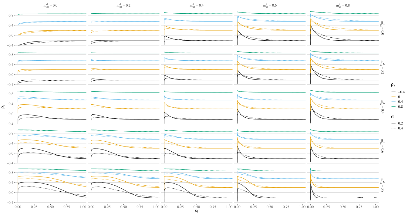
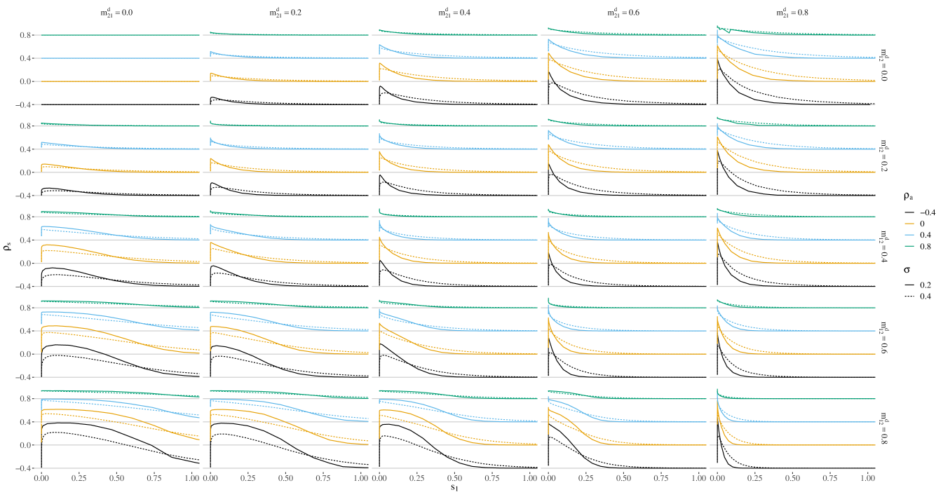
One of the central results of this paper is given by the Theorem 2; i.e., $\rho^{s}\geq\rho$ for two firms. Here, we illustrate it numerically by plotting the equity correlation for different values of asset correlations, initial prices, volatilities and cross-holding fractions. For the sake of simplicity, we consider cross-holdings of debt only ( $\bm{M}^{s}=\bm{0}$ ) and symmetric initial conditions for the assets¹¹1Thus, the both firms assets have the same spot value, but are still log-normally distributed at maturity. The case of comonotonic asset endowments as considered by Banerjee \BBA Feinstein (\APACyear2021) corresponds to the trivial case of fully correlated assets, i.e., $\rho=1$ , and thus $\rho_{s}=1$ as well., i.e., $\sigma_{1}=\sigma_{2}=\sigma$ and $a_{\text{1,0}}=a_{2,0}=a_{1,2}$ . Figure 1 show the resulting equity correlation as a function of firm 1’s equity²²2 Note that by symmetry of the setup, the corresponding figure for firm 2’s equity is just the mirror image, i.e., obtained by exchanging $M_{12}^{d}$ and $M_{21}^{d}$ ., for different debt cross-holding fractions, asset correlations and volatilities. Here, the subplots correspond to cross-holding fractions of $M_{12}^{d}=0,0.2,\ldots,0.8$ (vertical) and $M_{21}^{d}=0,0.2,\ldots,0.8$ (horizontal). Furthermore, solid lines represent an asset volatility value of $0.2$ while dotted lines a volatility value of 0.4. The colors correspond to different values of asset correlations $\rho_{a}=\left\{-0.4,0,0.4,0.8\right\}$ . As proved above (page • ‣ 4.2.2), in case of no cross-holdings (left and upper subplot) we find $\rho^{s}=\rho$ . In contrast, with cross-holdings the equity correlation shows a marked increase above the asset correlations until the equity reaches essentially zero. Most notable, even for anti-correlated business asset ( $\rho_{a}=-0.4$ ) the firm’s equities exhibit positive correlations for sufficiently large cross-holding fractions and stressed firm equities, i.e., during crises times with correspondingly low asset values. Similar effects are also observed for asymmetric asset values and with additional equity cross-holdings (as shown in appendix B).

Refer to caption — Figure 1: Equity correlations as function of firm 1’s equity value $s_{1,0}$ , for different debt cross-holding fractions, asset correlations and volatilities.

5 Summary

We have used a financial network with cross-holdings to model the complex interlinkages around the financial firms and we put the accent in the study of the correlation of their derivatives. In fact, we uncover the capabilities of the Suzuki model to address the non-constant behavior of the correlation observed in the equity market; even from constant values of the business asset correlations. We shown mathematically, that the correlation among equities depends on the structure of the financial networks. Furthermore, we demonstrate analytically for the two firms case, the equity correlation is never lower than the unconditional correlation of the asset returns. Besides, the numerical simulations shows the power of the network approach too explain structurally the increase in correlation under crisis.

Acknowledgement

This work has been supported by DFG BE 7225/1–1.

References

Adams \BOthers. (\APACyear2017) \APACinsertmetastaradams2017correlations{APACrefauthors}Adams, Z., Füss, R.\BCBL \BBA Glück, T. \APACrefYearMonthDay2017. \BBOQ\APACrefatitleAre correlations constant? Empirical and theoretical results on popular correlation models in finance Are correlations constant? Empirical and theoretical results on popular correlation models in finance.\BBCQ \APACjournalVolNumPagesJournal of Banking & Finance849–24. \PrintBackRefs\CurrentBib
Ang \BBA Chen (\APACyear2002) \APACinsertmetastarang2002asymmetric{APACrefauthors}Ang, A.\BCBT \BBA Chen, J. \APACrefYearMonthDay2002. \BBOQ\APACrefatitleAsymmetric correlations of equity portfolios Asymmetric correlations of equity portfolios.\BBCQ \APACjournalVolNumPagesJournal of Financial Economics633443–494. \PrintBackRefs\CurrentBib
Baig \BBA Goldfajn (\APACyear1999) \APACinsertmetastarBaig1999{APACrefauthors}Baig, T.\BCBT \BBA Goldfajn, I. \APACrefYearMonthDay1999Jun01. \BBOQ\APACrefatitleFinancial Market Contagion in the Asian Crisis Financial market contagion in the Asian crisis.\BBCQ \APACjournalVolNumPagesIMF Staff Papers462167–195. {APACrefDOI} \doi10.2307/3867666 \PrintBackRefs\CurrentBib
Banerjee \BBA Feinstein (\APACyear2021) \APACinsertmetastarfeinstein2021{APACrefauthors}Banerjee, T.\BCBT \BBA Feinstein, Z. \APACrefYearMonthDay2021. \BBOQ\APACrefatitlePricing of debt and equity in a financial network with comonotonic endowments Pricing of debt and equity in a financial network with comonotonic endowments.\BBCQ \APACjournalVolNumPagesarXiv:1810.01372. \PrintBackRefs\CurrentBib
Broadie \BBA Glasserman (\APACyear1996) \APACinsertmetastarbroadie1996estimating{APACrefauthors}Broadie, M.\BCBT \BBA Glasserman, P. \APACrefYearMonthDay1996. \BBOQ\APACrefatitleEstimating security price derivatives using simulation Estimating security price derivatives using simulation.\BBCQ \APACjournalVolNumPagesManagement Science422269–285. \PrintBackRefs\CurrentBib
Caccioli \BOthers. (\APACyear2018) \APACinsertmetastarcaccioli2018network{APACrefauthors}Caccioli, F., Barucca, P.\BCBL \BBA Kobayashi, T. \APACrefYearMonthDay2018. \BBOQ\APACrefatitleNetwork models of financial systemic risk: A review Network models of financial systemic risk: A review.\BBCQ \APACjournalVolNumPagesJournal of Computational Social Science1181–114. \PrintBackRefs\CurrentBib
Choi \BBA Shin (\APACyear2019) \APACinsertmetastarchoi2019self{APACrefauthors}Choi, J\BHBIE.\BCBT \BBA Shin, D\BPBIW. \APACrefYearMonthDay2019. \BBOQ\APACrefatitleA self-normalization test for correlation change A self-normalization test for correlation change.\BBCQ \APACjournalVolNumPagesEconomics Letters. \PrintBackRefs\CurrentBib
Cifuentes \BOthers. (\APACyear2005) \APACinsertmetastarcifuentes2005liquidity{APACrefauthors}Cifuentes, R., Ferrucci, G.\BCBL \BBA Shin, H\BPBIS. \APACrefYearMonthDay2005. \BBOQ\APACrefatitleLiquidity risk and contagion Liquidity risk and contagion.\BBCQ \APACjournalVolNumPagesJournal of the European Economic Association32-3556–566. \PrintBackRefs\CurrentBib
Cizeau \BOthers. (\APACyear2001) \APACinsertmetastarcizeau2001correlation{APACrefauthors}Cizeau, P., Potters, M.\BCBL \BBA Bouchaud, J\BHBIP. \APACrefYearMonthDay2001. \BBOQ\APACrefatitleCorrelation structure of extreme stock returns Correlation structure of extreme stock returns.\BBCQ \APACjournalVolNumPagesQuantitative Finance12217–222. \PrintBackRefs\CurrentBib
Cont \BBA Wagalath (\APACyear2013) \APACinsertmetastarcont2013running{APACrefauthors}Cont, R.\BCBT \BBA Wagalath, L. \APACrefYearMonthDay2013. \BBOQ\APACrefatitleRunning for the exit: distressed selling and endogenous correlation in financial markets Running for the exit: distressed selling and endogenous correlation in financial markets.\BBCQ \APACjournalVolNumPagesMathematical Finance234718–741. \PrintBackRefs\CurrentBib
De Bandt \BBA Hartmann (\APACyear2000) \APACinsertmetastarde2000systemic{APACrefauthors}De Bandt, O.\BCBT \BBA Hartmann, P. \APACrefYearMonthDay2000. \APACrefbtitleSystemic risk: A survey Systemic risk: A survey \APACbVolEdTRWorking Paper \BNUM 35. \APACaddressInstitutionFrankfurt am MainEuropean Central Bank. \PrintBackRefs\CurrentBib
Demetrescu \BBA Wied (\APACyear2019) \APACinsertmetastardemetrescu2019testing{APACrefauthors}Demetrescu, M.\BCBT \BBA Wied, D. \APACrefYearMonthDay2019. \BBOQ\APACrefatitleTesting for constant correlation of filtered series under structural change Testing for constant correlation of filtered series under structural change.\BBCQ \APACjournalVolNumPagesThe Econometrics Journal22110–33. \PrintBackRefs\CurrentBib
Eisenberg \BBA Noe (\APACyear2001) \APACinsertmetastareisenberg2001systemic{APACrefauthors}Eisenberg, L.\BCBT \BBA Noe, T\BPBIH. \APACrefYearMonthDay2001. \BBOQ\APACrefatitleSystemic risk in financial systems Systemic risk in financial systems.\BBCQ \APACjournalVolNumPagesManagement Science472236–249. \PrintBackRefs\CurrentBib
Elliott \BOthers. (\APACyear2014) \APACinsertmetastarelliott2014financial{APACrefauthors}Elliott, M., Golub, B.\BCBL \BBA Jackson, M. \APACrefYearMonthDay2014. \BBOQ\APACrefatitleFinancial networks and contagion Financial networks and contagion.\BBCQ \APACjournalVolNumPagesAmerican Economic Review104103115–53. \PrintBackRefs\CurrentBib
Elsinger (\APACyear2009) \APACinsertmetastarelsinger2009financial{APACrefauthors}Elsinger, H. \APACrefYearMonthDay2009. \APACrefbtitleFinancial Networks, Cross Holdings, and Limited Liability Financial Networks, Cross Holdings, and Limited Liability \APACbVolEdTRWorking Paper \BNUM 156. \APACaddressInstitutionOesterreichische Nationalbank. \PrintBackRefs\CurrentBib
Fischer (\APACyear2014) \APACinsertmetastarfischer2014no{APACrefauthors}Fischer, T. \APACrefYearMonthDay2014. \BBOQ\APACrefatitleNo-Arbitrage Pricing Under Systemic Risk: Accounting for Cross-Ownership No-arbitrage pricing under systemic risk: Accounting for cross-ownership.\BBCQ \APACjournalVolNumPagesMathematical Finance24197–124. \PrintBackRefs\CurrentBib
Gai \BBA Kapadia (\APACyear2010) \APACinsertmetastargai2010contagion{APACrefauthors}Gai, P.\BCBT \BBA Kapadia, S. \APACrefYearMonthDay2010. \BBOQ\APACrefatitleContagion in financial networks Contagion in financial networks.\BBCQ \APACjournalVolNumPagesProceedings of the Royal Society A: Mathematical, Physical and Engineering Sciences46621202401–2423. \PrintBackRefs\CurrentBib
Hain \BBA Fischer (\APACyear2015) \APACinsertmetastarHain2015{APACrefauthors}Hain, J.\BCBT \BBA Fischer, T. \APACrefYearMonthDay2015. \BBOQ\APACrefatitleValuation algorithms for structural models of financial interconnectedness Valuation algorithms for structural models of financial interconnectedness.\BBCQ \APACjournalVolNumPagesarXiv:1501.07402. \PrintBackRefs\CurrentBib
Halkin (\APACyear1974) \APACinsertmetastarhalkin1974implicit{APACrefauthors}Halkin, H. \APACrefYearMonthDay1974. \BBOQ\APACrefatitleImplicit functions and optimization problems without continuous differentiability of the data Implicit functions and optimization problems without continuous differentiability of the data.\BBCQ \APACjournalVolNumPagesSIAM Journal on Control122229–236. \PrintBackRefs\CurrentBib
Kalkbrener \BBA Packham (\APACyear2015) \APACinsertmetastarkalkbrener2015correlation{APACrefauthors}Kalkbrener, M.\BCBT \BBA Packham, N. \APACrefYearMonthDay2015. \BBOQ\APACrefatitleCorrelation under stress in normal variance mixture models Correlation under stress in normal variance mixture models.\BBCQ \APACjournalVolNumPagesMathematical Finance252426–456. \PrintBackRefs\CurrentBib
Karl \BBA Fischer (\APACyear2014) \APACinsertmetastarkarl2014cross{APACrefauthors}Karl, S.\BCBT \BBA Fischer, T. \APACrefYearMonthDay2014. \BBOQ\APACrefatitleCross-ownership as a structural explanation for over-and underestimation of default probability Cross-ownership as a structural explanation for over-and underestimation of default probability.\BBCQ \APACjournalVolNumPagesQuantitative Finance1461031–1046. \PrintBackRefs\CurrentBib
Kyle \BBA Xiong (\APACyear2001) \APACinsertmetastarkyle2001contagion{APACrefauthors}Kyle, A\BPBIS.\BCBT \BBA Xiong, W. \APACrefYearMonthDay2001. \BBOQ\APACrefatitleContagion as a wealth effect Contagion as a wealth effect.\BBCQ \APACjournalVolNumPagesThe Journal of Finance5641401–1440. \PrintBackRefs\CurrentBib
Lillo \BBA Mantegna (\APACyear2000) \APACinsertmetastarlillo2000symmetry{APACrefauthors}Lillo, F.\BCBT \BBA Mantegna, R\BPBIN. \APACrefYearMonthDay2000. \BBOQ\APACrefatitleSymmetry alteration of ensemble return distribution in crash and rally days of financial markets Symmetry alteration of ensemble return distribution in crash and rally days of financial markets.\BBCQ \APACjournalVolNumPagesThe European Physical Journal B-Condensed Matter and Complex Systems154603–606. \PrintBackRefs\CurrentBib
Longin \BBA Solnik (\APACyear2001) \APACinsertmetastarlongin2001extreme{APACrefauthors}Longin, F.\BCBT \BBA Solnik, B. \APACrefYearMonthDay2001. \BBOQ\APACrefatitleExtreme correlation of international equity markets Extreme correlation of international equity markets.\BBCQ \APACjournalVolNumPagesThe Journal of Finance562649–676. \PrintBackRefs\CurrentBib
Merton (\APACyear1974) \APACinsertmetastarmerton1974pricing{APACrefauthors}Merton, R\BPBIC. \APACrefYearMonthDay1974. \BBOQ\APACrefatitleOn the pricing of corporate debt: The risk structure of interest rates On the pricing of corporate debt: The risk structure of interest rates.\BBCQ \APACjournalVolNumPagesThe Journal of Finance292449–470. \PrintBackRefs\CurrentBib
Onnela \BOthers. (\APACyear2003) \APACinsertmetastaronnela2003dynamics{APACrefauthors}Onnela, J\BHBIP., Chakraborti, A., Kaski, K., Kertesz, J.\BCBL \BBA Kanto, A. \APACrefYearMonthDay2003. \BBOQ\APACrefatitleDynamics of market correlations: Taxonomy and portfolio analysis Dynamics of market correlations: Taxonomy and portfolio analysis.\BBCQ \APACjournalVolNumPagesPhysical Review E685056110. \PrintBackRefs\CurrentBib
Preis \BOthers. (\APACyear2012) \APACinsertmetastarpreis2012quantifying{APACrefauthors}Preis, T., Kenett, D\BPBIY., Stanley, H\BPBIE., Helbing, D.\BCBL \BBA Ben-Jacob, E. \APACrefYearMonthDay2012. \BBOQ\APACrefatitleQuantifying the behavior of stock correlations under market stress Quantifying the behavior of stock correlations under market stress.\BBCQ \APACjournalVolNumPagesScientific Reports2752. \PrintBackRefs\CurrentBib
Sasidevan \BBA Bertschinger (\APACyear2019) \APACinsertmetastarsasidevan2019systemic{APACrefauthors}Sasidevan, V.\BCBT \BBA Bertschinger, N. \APACrefYearMonthDay2019. \BBOQ\APACrefatitleSystemic risk: Fire-walling financial systems using network-based approaches Systemic risk: Fire-walling financial systems using network-based approaches.\BBCQ \BIn A\BPBIS. Chakrabarti, L. Pichl\BCBL \BBA T. Kaizoji (\BEDS), \APACrefbtitleNetwork Theory and Agent-Based Modeling in Economics and Finance Network Theory and Agent-Based Modeling in Economics and Finance (\BPGS 313–330). \APACaddressPublisherSpringer. \PrintBackRefs\CurrentBib
Suzuki (\APACyear2002) \APACinsertmetastarsuzuki2002valuing{APACrefauthors}Suzuki, T. \APACrefYearMonthDay2002. \BBOQ\APACrefatitleValuing corporate debt: The effect of cross-holdings of stock and debt Valuing corporate debt: The effect of cross-holdings of stock and debt.\BBCQ \APACjournalVolNumPagesJournal of the Operations Research Society of Japan452123–144. \PrintBackRefs\CurrentBib

Appendix A Computing the Greeks

The Greeks quantify the sensitivities of derivative prices to changes in underlying parameters. Here, we consider first-order Greeks only. In particular, we compute the sensitivities of equity and debt prices accounting for cross-holdings with respect to current asset values $\Delta=\frac{\partial\bm{x}_{t}}{\partial\bm{a}_{t}}$ .

First, we recall the solution $\bm{A}_{t}$ of equation (18) as

\displaystyle\bm{A}_{t}

\displaystyle=\bm{a}_{0}e^{\left(r-\frac{1}{2}\operatorname{diag}(\bm{\sigma}^{2})\right)t+\operatorname{diag}(\bm{\sigma})\bm{W}_{t}}

(48)

where $\bm{a}_{0}>0$ denotes the initial value and $\bm{W}_{t}$ is multivariate normal distributed with mean $\bm{0}$ and covariance matrix $t\bm{C}$ . Note that $\bm{W}_{t}$ can be obtained from independent standard normal variates $\bm{Z}\sim\mathcal{N}(\bm{0},\bm{I}_{n\times n})$ as $\bm{W}_{t}=\sqrt{t}\bm{L}\bm{Z}$ with $\bm{L}^{T}\bm{L}=\bm{C}$ . We will use this representation in the next section to express the risk-neutral market value of equity and debt contracts as

\displaystyle\bm{x}_{t}=\mathbb{E}_{t}^{Q}[e^{-r\tau}\bm{x}^{*}\left(\bm{a}_{T}(\bm{Z})\right)]=\mathbb{E}_{t}^{Q}\left[e^{-r\tau}\bm{x}^{*}\left(\bm{a}_{t}e^{\left(r-\frac{1}{2}\bm{\sigma}^{2}\right)\tau+\sqrt{\tau}\operatorname{diag}(\bm{\sigma})\bm{L}\bm{Z}}\right)\right]\,.

(49)

A.1 Formal solution

Denoting all parameters of interest by $\bm{\theta}=(\bm{a}_{t},\bm{\sigma},r,\tau)^{T}$ and considering that the asset value $\bm{a}_{\tau}(Z;\theta)$ depends on the random variate $Z$ and these parameters, we need to compute the following derivatives

	$\displaystyle\frac{\partial}{\partial\bm{\theta}}\bm{x}_{t}$	$\displaystyle=\frac{\partial}{\partial\bm{\theta}}\mathbb{E}_{t}^{Q}[e^{-r\tau}\bm{x}^{*}(\bm{a}_{T}(Z;\theta))]$
		$\displaystyle=\mathbb{E}_{t}^{Q}\left[\left(\frac{\partial}{\partial\bm{\theta}}e^{-r\tau}\right)\bm{x}^{}(\bm{a}_{T}(Z;\theta))+e^{-r\tau}\left(\frac{\partial}{\partial\bm{\theta}}\bm{x}^{}(\bm{a}_{T}(Z;\theta))\right)\right]$		(50)

where we have used pathwise differentiation. Exchanging integration and differentiation requires some continuity conditions on $\bm{x}^{*}$ . In particular, \citeA[proposition 1]broadie1996estimating prove that pathwise differentiation is applicable for Lipschitz continuous functions.

Lemma 1.

The function $\bm{x}^{*}(\bm{a})$ is Lipschitz continuous with Lipschitz constant

\displaystyle L^{*}=(1-\max_{\bm{\xi}}\left\lVert\bm{K}_{\bm{\xi}}\right\rVert_{1})^{-1}

where

\displaystyle\bm{K}_{\bm{\xi}}

\displaystyle=\left(\begin{array}[]{cc}\operatorname{diag}(\bm{\xi})\bm{M}^{s}&\operatorname{diag}(\bm{\xi})\bm{M}^{d}\\ \operatorname{diag}(\bm{1}-\bm{\xi})\bm{M}^{s}&\operatorname{diag}(\bm{1}-\bm{\xi})\bm{M}^{d}\end{array}\right)\,.

Proof.

First, we observe that $\bm{g}$ is continuous and piecewise linear. In particular, we have

	$\displaystyle\left\lVert\bm{g}(\bm{a}_{1},\bm{x})-\bm{g}(\bm{a}_{2},\bm{x})\right\rVert_{1}$	$\displaystyle\leq\left\lVert\bm{a}_{1}-\bm{a}_{2}\right\rVert_{1}$
	$\displaystyle\left\lVert\bm{g}(\bm{a},\bm{x}_{1})-\bm{g}(\bm{a},\bm{x}_{2})\right\rVert_{1}$	$\displaystyle\leq\max_{\bm{\xi}}\left\lVert\bm{K}_{\bm{\xi}}\right\rVert_{1}\left\lVert\bm{x}_{1}-\bm{x}_{2}\right\rVert_{1}$

showing that $\bm{g}$ is Lipschitz continuous with respect to $\bm{a}$ and $\bm{x}$ .

Note that by assumption $1$ , we have $\left\lVert\bm{M}^{s}\right\rVert_{1},\left\lVert\bm{M}^{d}\right\rVert_{1}<1$ . Furthermore, the solvency indicator is either $\xi_{i}=1$ if bank $i$ is solvent or $\xi_{i}=0$ otherwise. Thus, it holds that $\left\lVert\bm{K}_{\bm{\xi}}\right\rVert_{1}<1,\forall\bm{\xi}\in\{0,1\}^{N}$ .

Then, we compute

	$\displaystyle\left\lVert\bm{x}^{}(\bm{a}_{1})-\bm{x}^{}(\bm{a}_{2})\right\rVert_{1}$	$\displaystyle=\left\lVert\bm{g}(\bm{a}_{1},\bm{x}^{}(\bm{a}_{1}))-\bm{g}(\bm{a}_{2},\bm{x}^{}(\bm{a}_{2}))\right\rVert_{1}$
		$\displaystyle=\left\lVert\bm{g}(\bm{a}_{1},\bm{x}^{}(\bm{a}_{1}))-\bm{g}(\bm{a}_{1},\bm{x}^{}(\bm{a}_{2}))+\bm{g}(\bm{a}_{1},\bm{x}^{}(\bm{a}_{2}))-\bm{g}(\bm{a}_{2},\bm{x}^{}(\bm{a}_{2}))\right\rVert_{1}$
		$\displaystyle\leq\left\lVert\bm{g}(\bm{a}_{1},\bm{x}^{}(\bm{a}_{1}))-\bm{g}(\bm{a}_{1},\bm{x}^{}(\bm{a}_{2}))\right\rVert_{1}+\left\lVert\bm{g}(\bm{a}_{1},\bm{x}^{}(\bm{a}_{2}))-\bm{g}(\bm{a}_{2},\bm{x}^{}(\bm{a}_{2}))\right\rVert_{1}$
		$\displaystyle\leq\max_{\bm{\xi}}\left\lVert\bm{K}_{\bm{\xi}}\right\rVert_{1}\left\lVert\bm{x}^{}(\bm{a}_{1}))-\bm{x}^{}(\bm{a}_{2}))\right\rVert_{1}+\left\lVert\bm{a}_{1}-\bm{a}_{2}\right\rVert_{1}$
	$\displaystyle\implies\left\lVert\bm{x}^{}(\bm{a}_{1})-\bm{x}^{}(\bm{a}_{2})\right\rVert_{1}$	$\displaystyle\leq(1-\max_{\bm{\xi}}\left\lVert\bm{K}_{\bm{\xi}}\right\rVert_{1})^{-1}\left\lVert\bm{a}_{1}-\bm{a}_{2}\right\rVert_{1}\;.$

∎

By the chain rule of differentiation we obtain

\displaystyle\frac{\partial}{\partial\bm{\theta}}\bm{x}^{*}(\bm{a}_{\tau}(Z;\theta))

\displaystyle=\frac{\partial}{\partial\bm{a}}\bm{x}^{*}(\bm{a})\mid_{\bm{a}=\bm{a}_{\tau}(Z;\theta)}\frac{\partial}{\partial\bm{\theta}}\bm{a}_{\tau}(Z;\theta)\,.

(51)

Note that $\frac{\partial}{\partial\bm{a}}\bm{x}^{*}(\bm{a})$ is the derivative of the fixed point solving (9). In order to compute it, we make use of the implicit function theorem. A version of the theorem by \citeAhalkin1974implicit is adopted to our notation:

Theorem 3.

Let $U\subset\mathbb{R}^{m},V\subset\mathbb{R}^{n}$ and $\bm{f}:U\times V\to\mathbb{R}^{n}$ a continuously differentiable function. Suppose that

\displaystyle\bm{f}(\bm{x}^{*},\bm{y}^{*})=\bm{0}

(52)

at a point $(\bm{x}^{*},\bm{y}^{*})\in U\times V$ and that the Jacobian matrices $\bm{J}_{\bm{f},\bm{x}}\bm{f}(\bm{x},\bm{y}),\bm{J}_{\bm{f},\bm{y}}\bm{f}(\bm{x},\bm{y})$ of partial derivatives exist at $(\bm{x}^{*},\bm{y}^{*})$ . Further, $\bm{J}_{\bm{f},\bm{y}}$ is invertible at this point. Then, there exists a neighborhood $U^{*}\subset U$ and a continuously differentiable function $\bm{h}:U^{*}\to\mathbb{R}^{n}$ with

\displaystyle\bm{h}(\bm{x}^{*})

\displaystyle=\bm{y}^{*}

(53)

and

\displaystyle\bm{f}(\bm{x},\bm{h}(\bm{x}))=\bm{0}\quad\forall\bm{x}\in U^{*}\,.

(54)

Moreover, the partial derivatives of $\bm{h}$ with respect to $\bm{x}\in U^{*}$ are given as

\displaystyle\frac{\partial}{\partial\bm{x}}\bm{h}(\bm{x})

\displaystyle=-\left[\bm{J}_{\bm{f},\bm{y}}\bm{f}(\bm{x},\bm{h}(\bm{x}))\right]_{n\times n}^{-1}\left[\frac{\partial}{\partial\bm{x}}\bm{f}(\bm{x},\bm{h}(\bm{x}))\right]_{n\times m}

(55)

As the function $\bm{g}(\bm{a},\bm{x})$ defined in equation (10) is Lipschitz continuous, it is almost everywhere differentiable. The partial derivatives are given by

$\displaystyle\frac{\partial}{\partial s_{j}}g_{i}^{s}(\bm{a},\bm{x})$	$\displaystyle=\left\{\begin{array}[]{rp{1cm}lcccc}M_{ij}^{s}&&\mbox{if firm $i$ is solvent}\\ 0&&\mbox{otherwise}\end{array}\right.$	(58)
$\displaystyle\frac{\partial}{\partial s_{j}}g_{i}^{r}(\bm{a},\bm{x})$	$\displaystyle=\left\{\begin{array}[]{rp{1cm}lcccc}0&&\mbox{if firm $i$ is solvent}\\ M_{ij}^{s}&&\mbox{otherwise}\end{array}\right.$	(61)
$\displaystyle\frac{\partial}{\partial r_{j}}g_{i}^{s}(\bm{a},\bm{x})$	$\displaystyle=\left\{\begin{array}[]{rp{1cm}lcccc}M_{ij}^{d}&&\mbox{if firm $i$ is solvent}\\ 0&&\mbox{otherwise}\end{array}\right.$	(64)
$\displaystyle\frac{\partial}{\partial r_{j}}g_{i}^{r}(\bm{a},\bm{x})$	$\displaystyle=\left\{\begin{array}[]{rp{1cm}lcccc}0&&\mbox{if firm $i$ is solvent}\\ M_{ij}^{d}&&\mbox{otherwise}\end{array}\right.$	(67)
$\displaystyle\frac{\partial}{\partial a_{j}}g_{i}^{s}(\bm{a},\bm{x})$	$\displaystyle=\left\{\begin{array}[]{rp{1cm}lcccc}\phantom{M}1&&\mbox{if $i=j$ and firm $i$ is solvent}\\ 0&&\mbox{otherwise}\end{array}\right.$	(70)
$\displaystyle\frac{\partial}{\partial a_{j}}g_{i}^{r}(\bm{a},\bm{x})$	$\displaystyle=\left\{\begin{array}[]{rp{1cm}lcccc}\phantom{M}0&&\mbox{if $i=j$ and firm $i$ is solvent}\\ 1&&\mbox{otherwise}\end{array}\right.\,.$	(73)

Here, a firm $i$ is solvent if its asset value $v_{i}$ is sufficient to repay its nominal debt $d_{i}$ , i.e. $v_{i}=a_{i}+\sum_{j=1}^{n}M_{ij}^{s}s_{j}+\sum_{j=1}^{n}M_{ij}^{d}r_{j}>d_{i}$ . The derivatives of $\bm{g}$ exist everywhere except for the boundary case $v_{i}=d_{i}$ . Defining the solvency vector $\bm{\xi}=(\mathbbm{1}_{v_{i}>d_{1}}(v_{1}),\ldots,\mathbbm{1}_{v_{n}>d_{n}}(v_{n}))$ , the partial derivatives of $\bm{g}$ with respect to $\bm{x}$ can be collected in a matrix as follows

	$\displaystyle\frac{\partial}{\partial\bm{x}}\bm{g}(\bm{a},\bm{x})$	$\displaystyle=\left[\begin{array}[]{ccc}\operatorname{diag}(\bm{\xi})\bm{M}^{s}&&\operatorname{diag}(\bm{\xi})\bm{M}^{d}\\ \\ \operatorname{diag}(\bm{1}_{n}-\bm{\xi})\bm{M}^{s}&&\operatorname{diag}(\bm{1}_{n}-\bm{\xi})\bm{M}^{d}\end{array}\right]$		(77)
		$\displaystyle=\operatorname{diag}\left((\bm{\xi};\bm{1}_{n}-\bm{\xi})\right)\left[\begin{array}[]{ccc}\bm{M}^{s}&&\bm{M}^{d}\\ \\ \bm{M}^{s}&&\bm{M}^{d}\end{array}\right]$		(81)

Thus, defining $\bm{f}(\bm{a},\bm{x})=\bm{x}-\bm{g}(\bm{a},\bm{x})$ we obtain by the implicit function theorem 3

Corollary 1.

The partial derivatives of $\bm{x}^{*}(\bm{a})$ are given by

\displaystyle\frac{\partial}{\partial\bm{a}}\bm{x}^{*}(\bm{a})

\displaystyle=\left[\bm{I}_{2n\times 2n}-\frac{\partial}{\partial\bm{x}}\bm{g}(\bm{a},\bm{x})\right]^{-1}\left[\begin{array}[]{c}\operatorname{diag}(\bm{\xi})\\ \\ \operatorname{diag}(\bm{1}_{n}-\bm{\xi})\end{array}\right]

(85)

Proof.

Use that $\frac{\partial}{\partial\bm{x}}\bm{f}(\bm{a},\bm{x})=\bm{I}_{2n\times 2n}-\frac{\partial}{\partial\bm{x}}\bm{g}(\bm{a},\bm{x})$ and $\frac{\partial}{\partial\bm{a}}\bm{f}(\bm{a},\bm{x})=-\frac{\partial}{\partial\bm{a}}\bm{g}(\bm{a},\bm{x})$ . Then, the result follows from theorem 3 and $\frac{\partial}{\partial\bm{a}}\bm{g}(\bm{a},\bm{x})=\left[\begin{array}[]{c}\operatorname{diag}(\bm{\xi})\\ \operatorname{diag}(\bm{1}_{n}-\bm{\xi})\end{array}\right]$ . As explained below, assumption 1 ensures that $\frac{\partial}{\partial\bm{x}}\bm{f}(\bm{a},\bm{x})$ is invertible as required. ∎

Finally, combining equation (50) and (51) with corollary 1 we formally compute the network Greeks as

	$\displaystyle\frac{\partial}{\partial\bm{\theta}}\bm{x}_{t}$	$\displaystyle=\mathbb{E}_{t}^{Q}\left[\left(\frac{\partial}{\partial\bm{\theta}}e^{-r\tau}\right)\bm{x}^{*}(\bm{a}_{T}(Z;\theta))\right.$
		$\displaystyle\phantom{=}\left.+e^{-r\tau}\left[\bm{I}_{2n\times 2n}-\frac{\partial}{\partial\bm{x}}\bm{g}(\bm{a},\bm{x})\right]^{-1}\left[\begin{array}[]{c}\operatorname{diag}(\bm{\xi})\\ \\ \operatorname{diag}(\bm{1}_{n}-\bm{\xi})\end{array}\right]\frac{\partial}{\partial\bm{\theta}}\bm{a}_{T}(Z;\theta)\right]$		(89)

where the expectation is well-defined as the derivatives exist almost everywhere, i.e. except for a set of measure zero.

A.2 Two bank Delta

In case of two banks, the network Delta, i.e. $\bm{\Delta}=\frac{\partial\bm{x}_{t}}{\partial\bm{a}_{t}}$ , can be computed explicitly. First, we drop the time index $t$ to ease notation and denote firm values (of equity and debt) and asset prices at time $t$ as $\bm{x}=(s_{1},s_{2},r_{1},r_{2})$ and $\bm{a}=(a_{1},a_{2})$ respectively. Then, using that $\frac{\partial}{\partial\bm{a}}e^{-r\tau}=\bm{0}$ and

	$\displaystyle\frac{\partial}{\partial\bm{a}}\bm{A}_{T}$	$\displaystyle=\frac{\partial}{\partial\bm{a}}\bm{a}\;e^{\left(r-\frac{1}{2}\operatorname{diag}(\bm{\sigma}^{2})\right)(T-t)+\operatorname{diag}(\bm{\sigma})\bm{W}_{T}}$
		$\displaystyle=\bm{I}\;e^{\left(r-\frac{1}{2}\operatorname{diag}(\bm{\sigma}^{2})\right)(T-t)+\operatorname{diag}(\bm{\sigma})\bm{W}_{T}}$	$\displaystyle=\left(\begin{array}[]{cc}\frac{A_{1,T}}{a_{1}}&0\\ 0&\frac{A_{2,T}}{a_{2}}\end{array}\right)$

from equation (19) with suitably shifted time indices, equation (89) simplifies to

\displaystyle\frac{\partial}{\partial\bm{a}}\bm{x}_{t}

\displaystyle=\mathbb{E}_{t}^{Q}\left[e^{-r\tau}\left[\bm{I}_{4\times 4}-\frac{\partial}{\partial\bm{x}}\bm{g}(\bm{a},\bm{x})\right]^{-1}\left[\begin{array}[]{c}\operatorname{diag}(\bm{\xi})\\ \\ \operatorname{diag}(\bm{1}-\bm{\xi})\end{array}\right]\left(\begin{array}[]{cc}\frac{A_{1,T}}{a_{1}}&0\\ 0&\frac{A_{2,T}}{a_{2}}\end{array}\right)\right]

Furthermore, we find from equation (77) that

\displaystyle\bm{I}_{4\times 4}-\frac{\partial}{\partial\bm{x}}\bm{g}(\bm{a},\bm{x})

\displaystyle=\left(\begin{array}[]{cccc}1&-\xi_{1}M^{s}_{12}&0&-\xi_{1}M^{d}_{12}\\ -\xi_{2}M^{s}_{21}&1&-\xi_{2}M^{d}_{21}&0\\ 0&-(1-\xi_{1})M^{s}_{12}&1&-(1-\xi_{1})M^{d}_{12}\\ -(1-\xi_{2})M^{s}_{21}&0&-(1-\xi_{2})M^{d}_{21}&1\end{array}\right)

Thus, the matrix is piecewise constant on each solvency region and $\bm{\Delta}$ can be found in all four cases. For illustration, we detail the case $\xi_{1}=\xi_{2}=1$ , i.e. both banks solvent:

	$\displaystyle\left[\bm{I}_{4\times 4}-\frac{\partial}{\partial\bm{x}}\bm{g}(\bm{a},\bm{x})\right]^{-1}\left[\begin{array}[]{c}\operatorname{diag}(\bm{\xi})\\ \\ \operatorname{diag}(\bm{1}-\bm{\xi})\end{array}\right]\left(\begin{array}[]{cc}\frac{A_{1,T}}{a_{1}}&0\\ 0&\frac{A_{2,T}}{a_{2}}\end{array}\right)$	$\displaystyle=\left(\begin{array}[]{cccc}1&-M^{s}_{12}&0&-M^{d}_{12}\\ -M^{s}_{21}&1&-M^{d}_{21}&0\\ 0&0&1&0\\ 0&0&0&1\end{array}\right)^{-1}\left(\begin{array}[]{cc}1&0\\ 0&1\\ 0&0\\ 0&0\end{array}\right)\left(\begin{array}[]{cc}\frac{A_{1,T}}{a_{1}}&0\\ 0&\frac{A_{2,T}}{a_{2}}\end{array}\right)$
		$\displaystyle=\left(\begin{array}[]{cccc}\frac{1}{1-M^{s}_{12}M^{s}_{22}}&\frac{M^{s}_{12}}{1-M^{s}_{12}M^{s}_{22}}&0&0\\ \frac{M^{s}_{21}}{1-M^{s}_{12}M^{s}_{22}}&\frac{1}{1-M^{s}_{12}M^{s}_{22}}&0&0\\ 0&0&1&0\\ 0&0&0&1\end{array}\right)\left(\begin{array}[]{cc}1&0\\ 0&1\\ 0&0\\ 0&0\end{array}\right)\left(\begin{array}[]{cc}\frac{A_{1,T}}{a_{1}}&0\\ 0&\frac{A_{2,T}}{a_{2}}\end{array}\right)$
		$\displaystyle=\left(\begin{array}[]{cc}\frac{1}{1-M^{s}_{12}M^{s}_{22}}\frac{A_{1,T}}{a_{1}}&\frac{M^{s}_{12}}{1-M^{s}_{12}M^{s}_{22}}\frac{A_{2,T}}{a_{2}}\\ \frac{M^{s}_{21}}{1-M^{s}_{12}M^{s}_{22}}\frac{A_{1,T}}{a_{1}}&\frac{1}{1-M^{s}_{12}M^{s}_{22}}\frac{A_{2,T}}{a_{2}}\\ 0&0\\ 0&0\end{array}\right)$

containing the $\Delta$ ’s for equity (top) and debt (bottom) respectively. Note that the equity $\Delta$ ’s correspond to the terms for solvency region $\Xi_{ss}$ in equations (37) – (43).

Here, we have used that the inverse of a block matrix can be expressed via the Schur complement as

\displaystyle\left(\begin{array}[]{cc}\bm{B}_{11}&\bm{B}_{12}\\ \bm{B}_{21}&\bm{B}_{22}\end{array}\right)^{-1}

\displaystyle=\left(\begin{array}[]{cc}\bm{I}&\bm{0}\\ -\bm{B}_{22}^{-1}\bm{B}_{21}&\bm{I}\end{array}\right)\left(\begin{array}[]{cc}(\bm{B}_{11}-\bm{B}_{12}\bm{B}_{22}^{-1}\bm{B}_{21})^{-1}&\bm{0}\\ \bm{0}&\bm{B}_{22}^{-1}\end{array}\right)\left(\begin{array}[]{cc}\bm{I}&-\bm{B}_{12}\bm{B}_{22}^{-1}\\ \bm{0}&\bm{I}\end{array}\right)\;.

As in our case, $\bm{B}_{11}=\bm{I}-\bm{M}^{s},\bm{B}_{12}=\bm{M}^{d},\bm{B}_{21}=\bm{0}$ and $\bm{B}_{22}=\bm{I}$ , we obtain

\displaystyle\left(\begin{array}[]{cc}\bm{I}&\bm{0}\\ \bm{0}&\bm{I}\end{array}\right)\left(\begin{array}[]{cc}(\bm{I}-\bm{M}^{s})^{-1}&\bm{0}\\ \bm{0}&\bm{I}\end{array}\right)\left(\begin{array}[]{cc}\bm{I}&-\bm{M}^{d}\bm{I}\\ \bm{0}&\bm{I}\end{array}\right)

\displaystyle=\left(\begin{array}[]{cc}(\bm{I}-\bm{M}^{s})^{-1}&\bm{0}\\ \bm{0}&\bm{I}\end{array}\right)

and the above results follows from

\displaystyle\left(\begin{array}[]{cc}1&-M^{s}_{12}\\ -M^{s}_{21}&1\end{array}\right)^{-1}

\displaystyle=\frac{1}{1-M^{s}_{12}M^{s}_{22}}\left(\begin{array}[]{cc}1&M^{s}_{12}\\ M^{s}_{21}&1\end{array}\right)\;.

The $\Delta$ ’s on the other three solvency regions can be found analogously and are ommitted for brevity.

Appendix B Additional figures

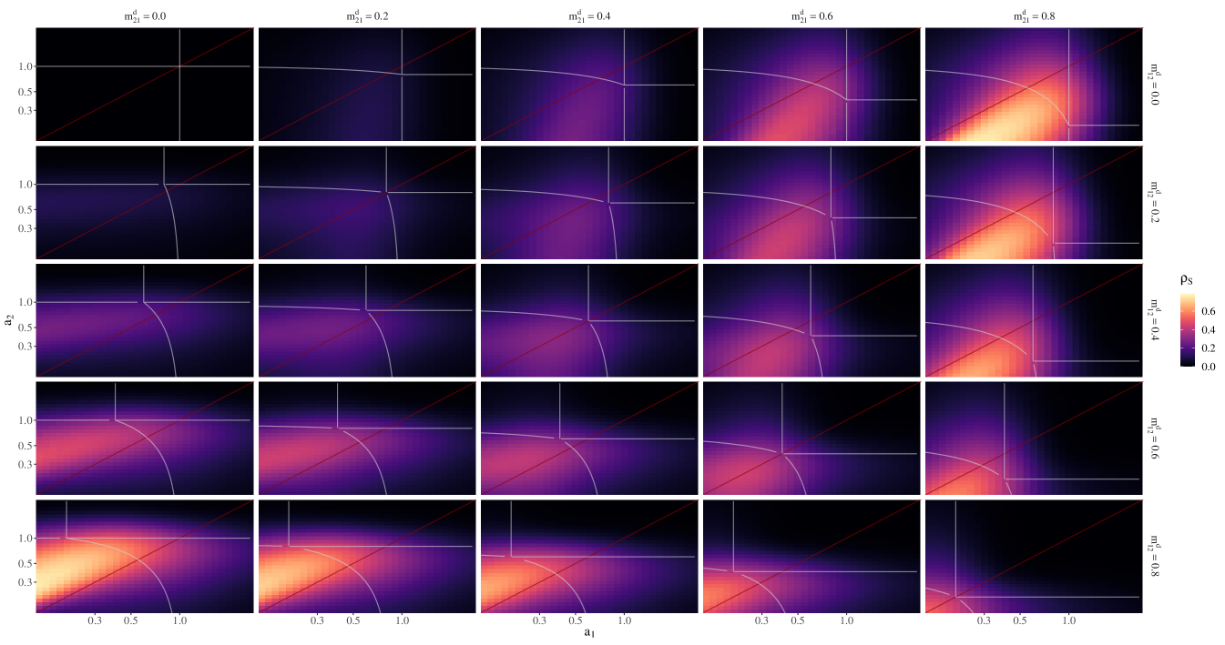
Markedly rising equity correlations at sufficiently low asset values are also observed with additional equity cross-holdings of 10% (figure 2) and asymmetric asset values (figure 3). As the figure is no longer symmetric with respect to the firms equity values, we show the initial values of $a_{1}$ and $a_{2}$ (in log-scale) instead. The Suzuki areas, i.e., default boundaries, are indicated by grey lines and the equity correlations are color coded. Again, at sufficiently large debt cross-holding fractions a marked increase in equity correlations is observed, especially in the $\Xi_{dd}$ Suzuki area, i.e., during crisis.

$\displaystyle\frac{\Delta_{12}}{\Delta_{11}}$	$\displaystyle=\frac{\pi_{ss}\frac{1}{1-M_{12}^{s}M_{21}^{s}}M_{12}^{s}\mathbb{E}^{Q}\left[\frac{A_{2,T}}{a_{2}}\bigm{\|}\Xi_{ss}\right]+\pi_{sd}\frac{1}{1-M_{12}^{d}M_{21}^{s}}M_{12}^{d}\mathbb{E}^{Q}\left[\frac{A_{2,T}}{a_{2}}\bigm{\|}\Xi_{sd}\right]}{\pi_{ss}\frac{1}{1-M_{12}^{s}M_{21}^{s}}\mathbb{E}^{Q}\left[\frac{A_{1,T}}{a_{1}}\bigm{\|}\Xi_{ss}\right]+\pi_{sd}\frac{1}{1-M_{12}^{d}M_{21}^{s}}\mathbb{E}^{Q}\left[\frac{A_{1,T}}{a_{1}}\bigm{\|}\Xi_{sd}\right]}$
	$\displaystyle=\frac{\frac{1}{1-M_{12}^{s}M_{21}^{s}}M_{12}^{s}\mathbb{E}^{Q}\left[\frac{A_{2,T}}{a_{2}}\bigm{\|}\Xi_{ss}\right]+\frac{\pi_{sd}}{\pi_{ss}}\frac{1}{1-M_{12}^{d}M_{21}^{s}}M_{12}^{d}\mathbb{E}^{Q}\left[\frac{A_{2,T}}{a_{2}}\bigm{\|}\Xi_{sd}\right]}{\frac{1}{1-M_{12}^{s}M_{21}^{s}}\mathbb{E}^{Q}\left[\frac{A_{1,T}}{a_{1}}\bigm{\|}\Xi_{ss}\right]+\frac{\pi_{sd}}{\pi_{ss}}\frac{1}{1-M_{12}^{d}M_{21}^{s}}\mathbb{E}^{Q}\left[\frac{A_{1,T}}{a_{1}}\bigm{\|}\Xi_{sd}\right]}$
	$\displaystyle\xrightarrow[a_{1},a_{2}\to\infty]{}M_{12}^{s}\frac{\mathbb{E}^{Q}\left[\frac{A_{2,T}}{a_{2}}\bigm{\|}\Xi_{ss}\right]}{\mathbb{E}^{Q}\left[\frac{A_{1,T}}{a_{1}}\bigm{\|}\Xi_{ss}\right]}$	(46)

	$\displaystyle\left\lVert\bm{x}^{}(\bm{a}_{1})-\bm{x}^{}(\bm{a}_{2})\right\rVert_{1}$	$\displaystyle=\left\lVert\bm{g}(\bm{a}_{1},\bm{x}^{}(\bm{a}_{1}))-\bm{g}(\bm{a}_{2},\bm{x}^{}(\bm{a}_{2}))\right\rVert_{1}$
		$\displaystyle=\left\lVert\bm{g}(\bm{a}_{1},\bm{x}^{}(\bm{a}_{1}))-\bm{g}(\bm{a}_{1},\bm{x}^{}(\bm{a}_{2}))+\bm{g}(\bm{a}_{1},\bm{x}^{}(\bm{a}_{2}))-\bm{g}(\bm{a}_{2},\bm{x}^{}(\bm{a}_{2}))\right\rVert_{1}$
		$\displaystyle\leq\left\lVert\bm{g}(\bm{a}_{1},\bm{x}^{}(\bm{a}_{1}))-\bm{g}(\bm{a}_{1},\bm{x}^{}(\bm{a}_{2}))\right\rVert_{1}+\left\lVert\bm{g}(\bm{a}_{1},\bm{x}^{}(\bm{a}_{2}))-\bm{g}(\bm{a}_{2},\bm{x}^{}(\bm{a}_{2}))\right\rVert_{1}$
		$\displaystyle\leq\max_{\bm{\xi}}\left\lVert\bm{K}_{\bm{\xi}}\right\rVert_{1}\left\lVert\bm{x}^{}(\bm{a}_{1}))-\bm{x}^{}(\bm{a}_{2}))\right\rVert_{1}+\left\lVert\bm{a}_{1}-\bm{a}_{2}\right\rVert_{1}$
	$\displaystyle\implies\left\lVert\bm{x}^{}(\bm{a}_{1})-\bm{x}^{}(\bm{a}_{2})\right\rVert_{1}$	$\displaystyle\leq(1-\max_{\bm{\xi}}\left\lVert\bm{K}_{\bm{\xi}}\right\rVert_{1})^{-1}\left\lVert\bm{a}_{1}-\bm{a}_{2}\right\rVert_{1}\;.$