CrossGen: Learning and Generating Cross Fields for Quad Meshing
Abstract.
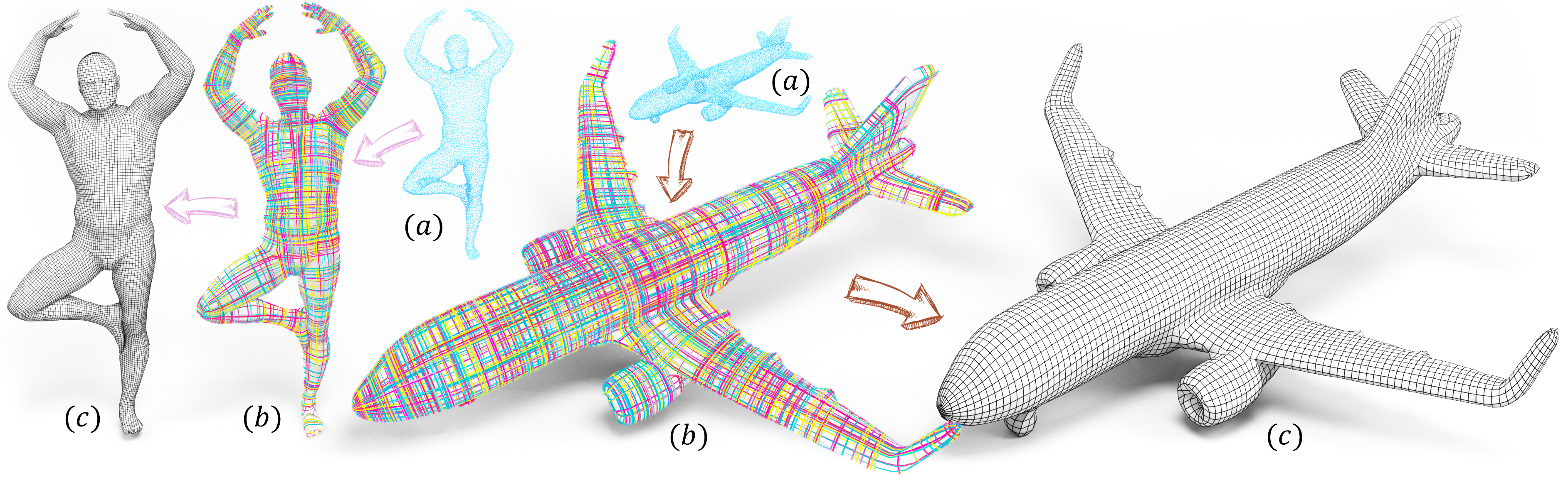
Cross fields play a critical role in various geometry processing tasks, especially for quad mesh generation. Existing methods for cross field generation often struggle to balance computational efficiency with generation quality, using slow per-shape optimization. We introduce CrossGen, a novel framework that supports both feed-forward prediction and latent generative modeling of cross fields for quad meshing by unifying geometry and cross field representations within a joint latent space. Our method enables extremely fast computation of high-quality cross fields of general input shapes, typically within one second without per-shape optimization. Our method assumes a point-sampled surface, or called a point-cloud surface, as input, so we can accommodate various different surface representations by a straightforward point sampling process. Using an auto-encoder network architecture, we encode input point-cloud surfaces into a sparse voxel grid with fine-grained latent spaces, which are decoded into both SDF-based surface geometry and cross fields (see the teaser figure). We also contribute a dataset of models with both high-quality signed distance fields (SDFs) representations and their corresponding cross fields, and use it to train our network. Once trained, the network is capable of computing a cross field of an input surface in a feed-forward manner, ensuring high geometric fidelity, noise resilience, and rapid inference. Furthermore, leveraging the same unified latent representation, we incorporate a diffusion model for computing cross fields of new shapes generated from partial input, such as sketches. To demonstrate its practical applications, we validate CrossGen on the quad mesh generation task for a large variety of surface shapes. Experimental results demonstrate that CrossGen generalizes well across diverse shapes and consistently yields high-fidelity cross fields, thus facilitating the generation of high-quality quad meshes.
1. Introduction
Cross fields are fundamental in various geometry processing tasks, such as quadrilateral (quad) mesh generation (Jakob et al., 2015; Huang et al., 2018; Pietroni et al., 2021; Bommes et al., 2009; Dielen et al., 2021; Bommes et al., 2013b; Zhang et al., 2020), surface subdivision (Loop and Schaefer, 2008; Shen et al., 2014), layout generation (Campen et al., 2012), and shape parameterization (T-spline design) (Campen and Zorin, 2017), as they provide a powerful way to capture the underlying structure and flow of surface geometry. By aligning with principal curvature directions and conforming to sharp feature edges or the boundaries of open surfaces, cross fields effectively capture the natural flow of the underlying geometry, leading to more coherent and visually consistent results.
The main driving force for cross field generation is the task of quad meshing, which plays a pivotal role in computer graphics, engineering, and scientific computing. From character animation and digital sculpting to physics simulation and architectural geometry, quad meshes offer benefits such as simpler subdivision schemes and compatibility with downstream applications such as parameterization and spline construction. A major factor determining the fidelity and adaptability of a quad mesh is the cross field (see Fig. 2). It is noted that better fields can produce quad meshes with fewer distortions, more uniform spacing, and improved alignment with intrinsic surface features (Vaxman et al., 2016; Pietroni et al., 2021).
Although high-quality cross fields offer clear advantages, generating cross fields that accurately capture the intrinsic geometry of complex shapes is non-trivial. Most methods rely on slow per-shape optimization, such as Dong et al. (2025) and Huang et al. (2018), which can take several minutes for a single shape. These methods do not generalize to new shapes without optimization. However, data-driven approaches for generalizable cross field generation remain under-explored. One closely related work is Dielen et al. (2021), which proposes a method specifically for learning directional fields for the human mesh category using a data-driven approach. This method is specifically designed and tested on a single category and relies on global shape encoding. Extending it to generalizable cross field generation across various shape categories is an open problem. These optimization-based methods or data-driven approaches are typically slow or lack demonstrated generalization ability across categories, limiting their practical utility.
In this work, we aim to address the above challenges by focusing on two core objectives: (1) Fast high-fidelity cross field generation, so cross fields can be computed in milliseconds without the need for slow iterative per-shape optimization; and (2) Generalization across a broad range of shape types, including smooth organic surfaces, common objects, CAD models, and surfaces with open boundaries.
To fulfill these objectives, we propose a novel framework, called CrossGen. The input to our method is assumed to a point-cloud surface, which can be a raw point cloud or points sampled from another surface representation, such as a triangle mesh surface. Hence we may also accommodate an input shape given in any surface representation since it can be converted to a point-cloud surface through sampling. Furthermore, we assume that each point of the input is associated with a surface normal vector, which is either provided directly or estimated using the method proposed by Xu et al. (2023). Our network simultaneously outputs a signed distance field (SDF) of the input shape and the cross field. The zero-level set of the SDF provides a continuous surface for extracting a quad mesh as guided by the output cross field. See the teaser figure for an illustration.
CrossGen adopts an auto-encoder architecture. The encoder transforms the input point clouds into a latent space composed of sparse grids of embeddings. These embeddings are then decoded into a high-resolution feature grid, which supports the simultaneous prediction of the SDF and cross field through two multi-layer perception (MLP) branches. Note that the encoder predominantly captures localized geometric details rather than global shape semantics, in order to enhance cross-categorical generalization capacity across diverse topological classes. Additionally, leveraging the same learned latent space, we explore the extension of our framework to generative modeling by incorporating a two-stage diffusion pipeline in the latent space. With this extension, the synthesis of novel 3D shapes and the computation of their cross fields are carried out in an end-to-end manner.
To train our network, we need a dataset of diverse shapes with annotations of paired SDF-based surfaces and high-quality cross fields. To the best of our knowledge, there is currently no publicly available dataset of this kind. Hence, we have made a diverse dataset of 3D shapes. For each shape, we compute an SDF to capture its geometry, along with a corresponding cross field aligned with principal curvature directions or sharp features. The resulting dataset comprises over 10,000 shapes, offering rich geometric and structural diversity to support robust and generalizable model training.
In summary, we make the following contributions:
-
•
Unified geometry representation. We develop a novel auto-encoder network as the backbone of CrossGen for robust learning of cross-fields of a large variety of input shapes. Specifically, the unique design of the encoder with a local perception field enables CrossGen to generalize well across diverse shape types and remain robust to out-of-domain inputs and rotational variations. For inference, CrossGen computes a cross-field within one second, several orders of magnitude faster over the state-of-the-art optimization-based methods.
-
•
Large-scale dataset. We contribute a training dataset of over 10,000 shapes annotated with high-quality SDFs and cross field, which is the first dataset of its kind.
-
•
Performance validation. We present extensive validation and comparisons of CrossGen with the existing methods to demonstrate the efficacy of CrossGen in terms of efficiency and quality of the cross fields and quad meshes computed.
We will publicly release both our dataset and code. In addition to high-quality SDFs and cross field pairs, the dataset will also include quad meshes extracted from the cross fields, facilitating further research and downstream applications.
2. Related Work
2.1. Cross Field Generation
There are numerous existing works (Sageman-Furnas et al., 2019; Diamanti et al., 2015; Panozzo et al., 2014; Ray et al., 2008; Hertzmann and Zorin, 2000; Vaxman et al., 2017) on generating cross fields of polygonal mesh surfaces. These efforts can be classified into two categories: optimization-based methods and data-driven methods.
Optimization-based Methods
Several methods utilize optimization to create cross fields. Mixed-Integer Quadrangulation (MIQ) (Bommes et al., 2009) initializes the cross field by aligning it with one edge of a triangular patch and subsequently applies a mixed integer optimization to ensure consistency of the cross fields across adjacent patches. While this method effectively preserves local consistency of the cross field, it fails to ensure global consistency across the entire 3D model. Power Fields (Knöppel et al., 2013) and PolyVectors (Diamanti et al., 2014) introduce convex smoothness energies for generating smooth N-RoSy fields. Power Fields (Knöppel et al., 2013) achieves global optimality through a convex formulation, but relies on a nonlinear transformation that can introduce additional singularities and geometric distortion. Instant Meshes (IM) (Jakob et al., 2015) and its variants (Huang et al., 2018; Pietroni et al., 2021) employ extrinsic energy to guide cross field optimization, enabling the generation of visually high-quality fields. However, their strong reliance on local information often undermines global consistency and leads to undesirable singularities.
Most of the above methods prioritize cross field smoothness at the expense of accurate alignment with principal curvature directions. Ideally, a high-quality cross field should strike a balance between smoothness and faithful alignment to principal curvature directions or sharp features. To this end, NeurCross (Dong et al., 2025) jointly optimizes the cross field and a neural signed distance field (SDF), where the zero-level set of the SDF serves as a proxy for the input surface. NeurCross (Dong et al., 2025) outperforms existing methods in terms of robustness to surface noise and geometric fluctuations, and alignment with curvature directions and sharp feature curves. However, its optimization process is computationally intensive, limiting its applicability in real-time or interactive scenarios. Moreover, all of these methods require per-shape optimization and thus not generalizable to new shapes. Our method, in contrast, is data-driven and therefore generalizable. It can generate cross fields for new shapes without the need for per-shape optimization.
Data-driven Methods
As a pioneering effort in utilizing deep learning for generalized generation, Dielen et al. (2021) introduces a fully automated, learning-based approach for predicting direction fields. By combining the information from a global network encoding the global semantics, a local network encoding the local geometry information, and a set of local reference frames indicating the local triangle position and rotation, it can infer a frame field in a feed-forward manner. However, this method relies on a global network (i.e., PointNet (Qi et al., 2017)) to encode the global domain knowledge of a single category (i.e., human-like body priors of quad meshes). Therefore it remains open as how to extend this method to shapes of different categories and even unseen categories. This method also assumes shapes are aligned in a canonical space, thus even small non-rigid changes, such as head rotations in human models, may disrupt the predictions.
The more recent work Point2Quad (Li et al., 2025) proposes a learning-based approach to extract quad meshes from point clouds by generating quad candidates via -NN grouping and filtering them using an MLP-based classifier. While promising, this candidate-driven approach requires post-processing heuristics and may produce non-watertight or non-manifold meshes. Furthermore, this method tends to produce extra undesired singularities, as shown by our test. In contrast, our method employs a sparse, locality-aware encoder that captures intrinsic geometric features without relying on global semantics. This design enables robust generalization across diverse shape categories and resilience to non-rigid deformations or pose variations, without requiring canonical alignment.
2.2. Cross Field Applications
Cross fields play a critical role in various geometry processing tasks. In quad mesh generation (Bommes et al., 2013a), they guide parameterization to ensure quad edges align with principal curvature directions, producing meshes that better preserve surface geometry and curvature, enhancing both aesthetic and functional performance. For surface subdivision (Shen et al., 2014), cross fields are used to construct the base mesh topology by decomposing the parameter space, automatically determining singular points, and ensuring tangential continuity across boundaries. Similarly, in T-spline design (Campen and Zorin, 2017), cross fields support the computation of global conformal parameterizations, from which aligned T-mesh domains are derived. These T-meshes enable the construction of smooth, piecewise rational surfaces for precise geometric modeling. In architectural geometry (Vouga et al., 2012), cross fields are employed to create specialized planar quad meshes, including conic meshes, that achieve structural stability and moment-free equilibrium in steel-glass assemblies. By aligning mesh edges with curvature fields, these designs ensure self-supporting frameworks with minimal forces on the glass, supporting efficient and elegant constructions. Together, these applications highlight the versatility and importance of cross fields in geometry processing and design. In this work, we focus specifically on quadrilateral meshing, which serves as a foundational component for many of these applications.
3. Method
Our goal is to efficiently generate a high-quality cross field of a given input point-cloud surface. We propose CrossGen based on an autoencoder architecture with novel designs of both encoder and decoder to enhance the generalization to unseen shapes. Fig. 3 shows the pipeline of CrossGen. In the following we describe the nework architecture, loss functions, and training dataset.
3.1. Network Architecture
Network Design
CrossGen adopts an autoencoder network architecture that takes a point-cloud surface as input and outputs the SDF of the input shape and a cross field on it. In order to ensure generalization across diverse shapes, we propose to use a shallow encoder based on a convolutional neural network (CNN) that focuses on local shape information without the need for learning global shape semantics. We then adopt a deep CNN decoder that takes into consideration of global geometry context for smooth and globally consistent generation of both SDFs and cross fields. We will shortly explain how to achieve these capabilities of learning local or global information using different ranges of the receptive field of a CNN.
Our design of using a local encoder and a global decoder is crucial for network generalization. On the one hand, shapes across different categories often appear globally different but share local similarities. For example, different local parts such as the chairs and the table may share similar local geometry, as illustrated in Fig. 4. Using a local geometry encoding mechanism helps to capture these local similar patterns, improving generalization across these diverse categories as demonstrated in (Mittal et al., 2022; Rombach et al., 2022). On the other hand, geometry decoding necessitates the integration of global geometric context to ensure smoothness and consistency in predictions, thereby enabling the learning of a more generalized representation.
Encoder
We adopt point clouds as the input surface format, which conveniently accommodates raw point-cloud surface as we as other surface representations, since any other surface representation can be converted to a point-cloud representation with a simple uniform sampling process. The resulting input to the encoder is a 3D point set. Let the input point set be denoted by , where each point is assumed to be associated with its corresponding surface unit normal vector as an input feature. These surface normal vectors can be extracted from the original continuous surface if provided as input, or estimated using Xu et al. (2023) for a raw point-cloud surface. These points are initially quantized into the vertices of a high-resolution cubic grid to ensure that the geometric details are well captured. This quantized data is subsequently encoded into 16-dimensional latent embeddings by a linear projection layer and fed into the encoder , which uses a sparse convolutional neural network (CNN) architecture (Choy et al., 2019) – a crucial choice for efficiently processing high-resolution 3D data while significantly reducing computational overhead.
The encoder consists of a sequence of convolutional layers and residual blocks that progressively downsample the input representation. As data propagates through the network, with the successive spatial resolutions of the feature maps being , , , , and , and corresponding feature dimensions being 16, 32, 64, 128, and 128. Each downsampling step uses a single convolutional layer to ensure a small receptive field and encourage the encoding of local geometric structures rather than global semantic features. At the network bottleneck, i.e. latent space, the 3D shape is compactly represented as a set of latent patch descriptors , where ( by default) denotes the feature dimensionality, as shown in Fig. 3 (b).
Decoder
The decoder , which also utilizes the sparse CNN architecture (Choy et al., 2019), comprises a sequence of convolutional upsampling layers and residual blocks, progressively increasing the spatial resolution of the feature maps to , , and , with the corresponding feature dimensions decreasing from 128 to 64 and then to 32. This process yields a high-resolution feature grid, as shown in Fig. 3 (c). At each resolution level, multiple convolutional layers are employed to expand the receptive field, enabling the propagation of geometric information to neighboring regions and enhancing feature aggregation for accurate SDF and cross field decoding.
\begin{overpic}[width=113.81102pt]{figs/receptive_field.jpg} \put(13.0,-10.0){\small{Small RF}} \put(65.0,-10.0){\small{Large RF}} \end{overpic}
Receptive Field
The receptive field (RF) of a CNN describes how much context of the input a network can “see” when making predictions at a given location. It defines the geometric context available for encoding the input point cloud surface and predicting the output, i.e. SDFs or cross fields. As shown in the inset for 2D illustration, smaller receptive fields focus on local details, while larger ones capture broader shape context. As discussed in Section 3.1, although shapes from different categories may vary globally, they often share local geometric similarities. To leverage this, we employ a small receptive field in the encoder to focus on local geometry (see Fig. 4). Meanwhile, we adopt a large receptive field in the decoder to aggregate broader context, which promotes smoothness and global coherence in the predicted cross fields.
SDF and Cross Field Modules
Subsequent to the construction of our high-resolution volumetric feature representation (see Fig. 3 (c)), we employ trilinear interpolation to extract two 32-dimensional feature vectors: one at the input points for cross field prediction, and another at query points for SDF prediction. The query set is sampled from a thin shell surrounding the zero-level set of the SDF, composed of points whose ground truth SDF magnitudes fall below a prescribed threshold (we use by default). Note that constitutes a proper subset of .
These interpolated features are fed into two distinct MLP decoders (see Fig. 5). One MLP decoder, , maps the feature vector at point to one cross field direction, while another, , maps the feature vector at point to a SDF value. In essence, decodes the interpolated feature vector at input points into directional cross field vectors, while interprets features in the thin shell into SDF values.
3.2. Loss Function
For training of CrossGen, we draw inspiration from previous works (Wang et al., 2025; Dong et al., 2025; Rombach et al., 2022) and design a composite loss function comprising four terms:
-
(1)
Occupancy Loss: Denoted , a term for multi-resolution volumetric fidelity that is applied to sparse grid representations across the successive layers of the decoder.
-
(2)
Cross Field Loss: Denoted , a term for enforcing cross field consistency at the input point cloud .
-
(3)
SDF Loss: Denoted , a term for predicting SDF values at queried points within the thin-shell space around the zero-level set of the SDF.
-
(4)
Latent Space Regularization: Denoted , a term that enforces structural coherence in the latent representation space for optimized feature encoding.
These individual loss terms and their corresponding weights are explained in detail below.
Occupancy Loss
In our pipeline, both the encoder and decoder adopt the sparse CNN architecture (Choy et al., 2019) for good computational and memory efficiency. In the encoder , empty voxels are directly removed during the downsampling process, keeping only the occupied regions for efficient feature extraction. During upsampling by the decoder , newly generated fine-grained sub-voxels, denoted as , are retained and marked as occupied only if they intersect with the thin shell region surrounding the zero-level set of the SDF; the rest are discarded.
To supervise voxel occupancy prediction at each resolution level of the output of the decoder , we introduce an occupancy loss , defined as the discrepancy between the predicted occupancy values and the ground truth occupancy labels .
| (1) |
where BCE(·) is the binary cross entropy, that is:
| (2) |
Cross Field Loss
Given a surface point , the cross field branch predicts one direction vector of the cross field at , denoted by . This predicted vector needs to be constrained to lie within the tangent plane at . Hence, we project onto the tangent plane defined by and its corresponding GT unit normal vector .
\begin{overpic}[width=113.81102pt]{figs/method_2.jpg} \put(55.0,38.0){$\boldsymbol{p}$} \put(70.0,62.0){$\mathcal{M}_{\text{cf}}(\boldsymbol{p})$} \put(81.5,34.0){$\bar{\boldsymbol{\alpha}}_{\boldsymbol{p}}$} \put(51.0,20.0){$\boldsymbol{\beta}_{\boldsymbol{p}}$} \put(44.5,69.0){$\boldsymbol{n}_{\boldsymbol{p}}$} \put(-3.0,46.0){\small{tangent plane}} \end{overpic}
As illustrated in the inset figure, we consider a local region centered at . Using the unit normal , we project the predicted vector onto the tangent plane, resulting in , a direction vector that lies within the tangent plane at . That is
| (3) |
We then normalize vector to obtain the unit vector , which represents one cross field direction at point predicted by our network. The second direction is computed as . Thus, the cross field at point predicted by our CrossGen is given by the pair , both of which are unit vectors lying in the tangent plane.
During training, to learn the cross field , we provide supervision by comparing it against the ground truth cross field . However, the exact correspondence between the two pairs is ambiguous due to their rotational symmetry. Following Dong et al. (2025), it suffices to require that one vector (i.e. ) from be aligned, being parallel or perpendicular, to both vectors in . It can be proved that this requirement is fulfilled if and only if attains its minimum value of 1 (Dong et al., 2025). Hence, the cross field loss term can be written as:
| (4) |
where denotes the absolute value.
SDF Loss
The SDF loss at point , measuring the discrepancy between the predicted value and the ground truth SDF , is defined as:
| (5) |
Latent Space Regularization
To prevent high variance and stabilize the latent space , we incorporate a KL divergence regularization term (Kingma and Welling, 2013), following (Mo et al., 2019; Rombach et al., 2022). This constrains the latent space distribution toward a standard normal distribution . Both empirical evidence and established theoretical results (Van Den Oord et al., 2017; Yan et al., 2022; Mittal et al., 2022; Kingma and Welling, 2013) demonstrate that this distributional constraint ensures a topologically coherent and smooth latent space (Mo et al., 2019; Rombach et al., 2022), substantially reducing information entropy during continuous shape parametrization transformations. Hence, we define the latent space regularization as follows:
| (6) |
where denotes the mean and the variance.
Total Loss
Finally, the overall training loss is defined as the sum of the occupancy loss, cross field loss, SDF loss, and the latent space regularization term:
| (7) |
where denote the corresponding weights of different loss terms to balance and stabilize the training process.
3.3. Dataset for Training
We have constructed a large-scale dataset of 3D shapes with ground-truth SDFs and cross fields for training our network and evaluating our method. To the best of our knowledge, there is no public dataset of 3D shapes that offers the ground truth of paired SDF and cross fields, which are needed for our training. For all the shapes in the dataset, their ground truth SDFs are computed using the Truncated Signed Distance Function (TSDF) (Werner et al., 2014), and their cross fields are computed using NeurCross (Dong et al., 2025).
To ensure geometric diversity for training a highly generalizable and robust network, the dataset contains 1,700 distinct shapes, including smooth organic surfaces, common object shapes (e.g. chairs, airplanes), and CAD models from the following sources:
-
(1)
Smooth Organic Shapes: These shapes are drawn from DeformingThings4D (Li et al., 2021), a synthetic dataset comprising 1,972 animation sequences across 31 categories of humanoid and animal models, with each category having 100 posed instances. We randomly select 10 models per category, yielding a total of 310 models.
-
(2)
Common Object Shapes: We sample 550 shapes from ShapeNetCore (Chang et al., 2015), which consists of 51,300 clean 3D models spanning 55 categories, by randomly selecting 10 shapes in each category, yielding 550 models. Additionally, we randomly select 530 models from Thingi10K (Zhou and Jacobson, 2016), a dataset known for its diverse collection of geometrically intricate 3D shapes.
-
(3)
CAD Models: We select 310 models from the ABC dataset (Koch et al., 2019), which comprises one million CAD models with explicitly parameterized curves and surfaces.
To enhance model resilience and promote orientation-invariant cross field predictions, the 1,700 distinct shapes in the dataset are augmented with random rotations, yielding over 10,000 shapes, and all the shapes are normalized to the cube to ensure consistent scaling across the shapes. Fig. 6 presents examples of cross field and SDF surfaces included in our dataset. This training dataset is partitioned using a 9:1 train-test split ratio.
3.4. Application to Quad Meshing
Quad Mesh Extraction
We now discuss how to use the cross field predicted by CrossGen to produce a quad mesh of the given shape. Since the input to CrossGen is a discrete point-cloud surface but existing quad mesh extraction methods require a mesh surface to operate on, we use the SDF predicted by CrossGen to provide such a continuous surface for quad meshing. Specially, we obtain a triangle mesh surface of the zero-level set of the predicted SDF using the Marching Cubes method (Lorensen and Cline, 1987). Then we compute the center points of the triangle faces and query their corresponding features from the high-resolution grid (Fig. 3 (c)). These features are then passed through the cross field branch to predict the cross fields. Finally, the predicted cross field and reconstructed surface mesh are used together to extract a field-aligned quad mesh. If the input shape is provided as a triangle mesh, we directly perform quad mesh extraction using the predicted cross field, without needing to reconstruct the surface through the SDF branch.
For quad mesh extraction, we implement a two-step pipeline similar to Dong et al. (2025); Bommes et al. (2009); Dielen et al. (2021). We first employ the global seamless parameterization algorithm from the libigl (Jacobson et al., 2017), which establishes parametric alignment with the predicted cross field. Then we utilize the libQEx (Ebke et al., 2013) to extract the quadrilateral tessellation from the parameterized representation.
Novel Quad Mesh Generation
With our unified geometry representation, 3D shapes are encoded into a sparse latent space that captures both geometric structure and cross field information. This latent space provides a natural foundation for generative modeling (Zheng et al., 2023). By incorporating a diffusion model within this latent, CrossGen can be extended to synthesize novel shapes and compute their cross fields in an end-to-end manner, providing an efficient way of quad meshing of the novel shapes. We provide further details and evaluations of this generative capability of CrossGen in Sec. 4.3.
4. Experiments
Implementation Details
We utilize distinct evaluation metrics to measure the quality of the generated cross field and the resulting quad mesh. (1) To evaluate the quality of the generated cross field, we employ two metrics: angular error (AE) relative to the principal curvature directions and computational time. The definition of AE is similar to that of Eq. 4, where . (2) To assess the quality of the generated quad meshes, we adopt five standard metrics following Huang et al. (2018) and Dong et al. (2025): area distortion (Area), angle distortion (Angle), number of singularities (# of Sings), Chamfer Distance (CD), and Jacobian Ratio (JR). Area distortion (Area), scaled by , measures the standard deviation of quadrilateral face areas, reflecting the uniformity of element sizing. Angle distortion (Angle), is computed as , where denotes interior angles and is the total number of angles; it captures deviations from the ideal right angles. Chamfer Distance (CD), scaled by and measured using the norm, evaluates geometric similarity between the predicted and ground truth surfaces. Jacobian Ratio (JR) quantifies local deformation uniformity by computing the ratio between the smallest and largest Jacobian determinants across element corners, ranging from 0 (degenerate) to 1 (perfect parallelogram). The number of singularities counts irregular vertices in the quad mesh, reflecting topological regularity.
During training, we uniformly sample 150,000 points from the ground-truth mesh as input and apply random point dropping as an augmentation strategy. We trained our model on a system equipped with 8 NVIDIA GeForce RTX 4090 GPUs, each with 24 GB of memory. The training was performed for 2,000 epochs using the Adam optimizer (Kingma and Jimmy, 2014) with a learning rate of and a batch size of 16. The full training process took approximately 15 days to converge on the complete dataset.
| Angular Error (AE) | Time (s) | ||
|---|---|---|---|
| all | high-res. | ||
| MIQ (Bommes et al., 2009) | 0.15 | 265.68 | 1201.38 |
| Power Fields (Knöppel et al., 2013) | 0.10 | 3.13 | 6.31 |
| PolyVectors (Diamanti et al., 2014) | 0.08 | 1.41 | 2.17 |
| IM (Jakob et al., 2015) | 0.06 | 2.13 | 5.28 |
| QuadriFlow (Huang et al., 2018) | 0.06 | 2.37 | 5.58 |
| NeurCross (Dong et al., 2025) | 0.04 | 360.58 | 912.46 |
| CrossGen (Ours) | 0.04 | 0.067 | 0.079 |
4.1. Comparisons
Quantitatively comparing our method is difficult because there are no publicly available learning-based methods for cross field generation in a feed-forward manner. However, to provide a comprehensive understanding of CrossGen’s performance, we compare it with several state-of-the-art optimization-based methods, including MIQ (Bommes et al., 2009), Power Fields (Knöppel et al., 2013), PolyVectors (Diamanti et al., 2014), IM (Jakob et al., 2015), QuadriFlow (Huang et al., 2018), and NeurCross (Dong et al., 2025). For all the methods, except MIQ (Bommes et al., 2009), we use their official open-source implementations with default parameters. As MIQ (Bommes et al., 2009) does not provide source code, we adopt its implementation from libigl (Jacobson et al., 2017). Since all the baselines take mesh surfaces input, we also test the option of using the input mesh at the stage of quad mesh extraction.
Cross Field Evaluation
Tab. 1 presents a quantitative comparison between our method and the baseline approaches. On the test data, our method and NeurCross (Dong et al., 2025) achieve the lowest angular error (AE) compared to the principal curvature directions, outperforming all other baselines. Benefiting from the direct inference design, CrossGen achieves the fastest average runtime, outperforming NeurCross (Dong et al., 2025) by approximately 5382 times on the full test data.
Note that only NeurCross (Dong et al., 2025) and our method are GPU-accelerated; all other baselines run on the CPU. To further evaluate performance under high-resolution inputs, we tested 50 randomly selected shapes from the test set, each with over 100,000 faces. As shown in Tab. 1, our method maintains a consistent runtime regardless of input resolution, demonstrating resolution-invariant efficiency. In contrast, all CPU-based methods show significantly increased runtime with higher resolution, while NeurCross (Dong et al., 2025), despite running on the GPU, is over 11,550 times slower than CrossGen and becomes increasingly constrained by computational overhead at higher resolutions. Fig. 7 presents a visual comparison of the cross fields generated by various methods.
| Area | Angle | # of Sings | CD | JR | |
| MIQ (Bommes et al., 2009) | 4.63 | 1.79 | 66.71 | 8.63 | 0.66 |
| Power Fields (Knöppel et al., 2013) | 4.55 | 1.77 | 85.41 | 8.76 | 0.72 |
| PolyVectors (Diamanti et al., 2014) | 4.53 | 1.72 | 87.21 | 8.75 | 0.71 |
| IM (Jakob et al., 2015) | 5.07 | 3.11 | 297.15 | 9.85 | 0.74 |
| QuadriFlow (Huang et al., 2018) | 5.04 | 2.28 | 98.31 | 28.38 | 0.79 |
| NeurCross (Dong et al., 2025) | 4.01 | 1.48 | 70.03 | 8.14 | 0.86 |
| CrossGen (Ours) | 4.32 | 1.60 | 80.65 | 8.45 | 0.83 |
| CrossGen∗ (Ours) | 4.28 | 1.55 | 78.17 | 8.23 | 0.84 |
Quad Mesh Evaluation
To evaluate the effectiveness of our method in downstream applications, we apply it to quadrilateral meshing tasks and compare the resulting mesh quality with optimization-based approaches in Tab. 2. Except for IM (Jakob et al., 2015) and QuadriFlow (Huang et al., 2018), all methods employ the same quad mesh extraction technique, libQEx (Ebke et al., 2013). Note that our method assumes a point-cloud surface as input, whereas the existing quad mesh extraction methods requires a triangle mesh as the base surface for parameterization and quad extraction. Since all the baseline methods operate on ground-truth triangle meshes, to evaluate our method comprehensively, we consider two settings in Tab. 2: (1) We test our model using the same ground-truth mesh as used the baseline methods as the base surface for querying the cross field and quad meshing, denoted as CrossGen∗. (2) Starting from point cloud input, we use the SDF branch to reconstruct a surface via Marching Cubes (Lorensen and Cline, 1987), which is then used as the base surface for quad meshing, denoted as CrossGen.
Tab. 2 shows the quantitative results comparing with baseline methods. Our method ranks second only to NeurCross across multiple evaluation metrics, outperforming all other baselines. We note that since NeurCross is used as the expert model to generate the GT data for training our CrossGen network, its performance is expected to be an upper bound for CrossGen’s performance. Besides, while both our method and NeurCross produce a higher number of singularities compared to MIQ (Bommes et al., 2009), our method achieves lower Jacobian Ratio (JR) values, indicating that MIQ (Bommes et al., 2009) tends to generate more distorted quadrilaterals. Fig. 8 presents a visual comparison, where our method produces high-quality and structurally consistent quadrilateral meshes, with results that are overall better or comparable to those of all the baseline methods. In addition, the setting CrossGen, which reconstructs the surface from point cloud inputs via the SDF branch, achieves results comparable to CrossGen∗, which uses the GT mesh as input. A visual comparison of the two settings is shown in Fig. 9. These results highlight the effectiveness of our SDF branch in producing high-quality surface geometry suitable for downstream quad meshing tasks.
Extraction Methods
We use existing methods to generate quad meshes guided by cross fields produced by CrossGen. There three widely adopted open-source extractors: the IM method (Jakob et al., 2015), libQEx (Ebke et al., 2013), and QuadWild (Pietroni et al., 2021). The IM extractor, specifically designed for IM (Jakob et al., 2015), leverages local parameterization to accelerate the extraction process. While it offers high efficiency, this speed often comes at the expense of mesh quality, typically resulting in increased singularities and non-quad face (e.g, triangle faces as shown in Fig. 8). In comparison, libQEx (Ebke et al., 2013) and QuadWild (Pietroni et al., 2021) tend to generate higher-quality quad meshes, though they are slower than IM. As noted in NeurCross (Dong et al., 2025), libQEx (Ebke et al., 2013) is particularly suited for quad meshing of free-form shapes, while QuadWild (Pietroni et al., 2021) is specifically designed to preserve sharp features and thus well-suited for CAD models and surfaces with open boundaries. Hence, we will test the performance of CrossGen in combination with both libQEx and QuadWild in the quad meshing task.
Fig. 10 shows quad meshes generated using libQEx (Ebke et al., 2013) and QuadWild (Pietroni et al., 2021), respectively, each driven by cross fields predicted by different baseline methods, as well as CrossGen. With each mesh extraction method fixed, the mesh quality is solely determined by the quality of the cross field provided. Fig. 10 shows that CrossGen consistently produces quad meshes of better quality than other baseline methods, indicating the superior quality of the cross field predicted by CrossGen.
Although CrossGen delivers extremely fast computation of cross fields, we have not accelerated the step of quad mesh extraction. Specifically, on our test dataset, libQEx (Ebke et al., 2013) and QuadWild (Pietroni et al., 2021) require an average of 40.81 seconds and 15.17 seconds, respectively, to extract a quad mesh from a given cross fields. Since the inference time for cross field prediction in our method is negligible, the total runtime from the input point cloud to the final quad mesh ranges from 15 to 41 seconds, depending on whether QuadWild (Pietroni et al., 2021) or libQEx (Ebke et al., 2013) is used to extract the quad mesh.
Comparison with Point2Quad
Point2Quad (Li et al., 2025) is a learning-based method that generates quad meshes directly from point clouds, primarily targeting CAD-like geometries. In their paper, only results on CAD shapes are presented, and no pretrained models are publicly available. Therefore, for comparison, we refer to the qualitative results provided in their official repository. As shown in Fig. 11, while Point2Quad can generate plausible quads on simple CAD shapes, it struggles to preserve global field smoothness, resulting in increased singularities in the generated quad meshes. In contrast, our method produces field-aligned quad meshes with improved regularity.
4.2. Analysis
Robustness to Missing and Sparse Input.
A key strength of CrossGen lies in its robustness to diverse point cloud inputs, enabled by the flexibility of using point clouds. Two common scenarios are incomplete and sparsely sampled data. In real-world settings, 3D scans frequently suffer from missing regions or low-resolution sampling. Unlike traditional methods that rely on complete surface meshes, CrossGen remains effective even when substantial portions of the input geometry are absent. By leveraging a locality-aware latent space, our model can infer global structure and cross fields from limited data. As shown in Fig. 12, CrossGen successfully reconstructs coherent surfaces and high-quality quad meshes even when inputs contain missing regions (b) or are reduced to as few as 10K points (c), demonstrating strong resilience and practicality in challenging data conditions.
Resistance to Noise
For point cloud inputs (Fig. 13 (a)), a triangle mesh surface is required to produce a quad mesh. One option is to use Poisson reconstruction (Kazhdan and Hoppe, 2013) to generate the surface (Fig. 13 (b)), but this approach can struggle to produce accurate results especially when the point cloud contains significant noise. In contrast, our method learns both SDF and cross field representations, enabling us to directly infer a high-quality SDF output from point cloud data via the SDF branch, even for noisy point clouds. We then extract the geometry surface using the Marching Cubes algorithm (Lorensen and Cline, 1987) (Fig. 13 (c)), sample points on the surface, and query the decoder’s feature volume to generate the corresponding cross field (Fig. 13 (d)) and extract the final quad mesh (Fig. 13 (e)). In Fig. 14, we further evaluate the robustness of our model under varying levels of Gaussian noise. Despite increasing noise, our method consistently produces smooth surfaces and coherent quad meshes, demonstrating strong resilience to input perturbations.
Robustness to Rotation
Another important feature of CrossGen is its robustness to random rotations. Unlike most existing methods that rely on shapes in a canonical pose, our method can process shapes with random pose inputs. By leveraging the learned local latent space representation, CrossGen can handle arbitrary orientations, making it more flexible and applicable in dynamic scenarios where the pose of the input shapes may vary without a requirement of a predefined orientation, as shown in Fig. 15.
Generalization to Out-of-domain Shapes
One more key strength of CrossGen is its ability to handle out-of-domain geometries and new shape categories. In our experiments, we tested our method on shapes from previously unseen categories in the training stage. Despite not being trained on these specific shapes, CrossGen successfully predicts high-quality cross fields, demonstrating its ability to generalize across a wide range of geometries and surface types, as shown in Fig. 16. This ability is crucial for real-world applications where new, previously unseen shapes may need to be processed without requiring retraining or fine-tuning on each new dataset.
Open-boundary Surfaces
Given a set of 3D points sampled from open-boundary surfaces, we first encode them into a high-resolution feature grid, then query the corresponding cross fields via the cross field branch, and finally extract the quad mesh using QuadWild (Pietroni et al., 2021). Fig. 17 presents quad mesh results generated by our method on the shapes with open boundaries. Although our training dataset does not explicitly include surfaces with open boundaries, we find that our model generalizes well to such surfaces. We attribute this capability to the use of a sparse and local encoder in our model’s encoding process. By focusing on local surface features, the encoder inherently emphasizes learning local geometry, enabling greater flexibility and generalization.
4.3. Quad Meshing of Novel Generated Shapes
To take advantage of the latent space learned by CrossGen, we have also explored the extension of CrossGen to generative modeling. Specifically, we design a two-stage diffusion pipeline that operates directly within this latent space, inspired by LAS-Diffusion (Zheng et al., 2023) and TRELLIS (Xiang et al., 2024). As illustrated in Fig. 18, our quad mesh generation pipeline begins with an occupancy diffusion model on sketch conditions (Fig. 18 (a)), which synthesizes a coarse voxel occupancy distribution in the latent space, providing a rough approximation of the global structure and topology of the target shape. In the second stage, conditioned on the coarse occupancy, a fine-grained latent diffusion model refines the representation by generating high-resolution latent embeddings that capture detailed geometry and cross field information necessary for downstream meshing (Fig. 18 (b)). Finally, the resulting latent codes are decoded into a cross field by the decoder (Fig. 18 (c)).
To demonstrate the effectiveness of generative capacity, we train the proposed two-stage diffusion pipeline on the full chair and airplane categories. Our method successfully generates cross fields that produce diverse and coherent quad meshes, consistently aligned with the input sketch conditions, as shown in Fig. 19. The results show that our latent space captures both global shape priors and cross field details necessary for high-quality quad meshing.
5. Ablation Study
To demonstrate the effectiveness of CrossGen, we conduct an ablation study to compare two different cross field representations. Existing methods, such as those proposed in Bommes et al. (2009), typically initialize a local coordinate system, predict the rotation angle of this coordinate system, and then generate a smooth cross field. In contrast, our approach simplifies this process by directly predicting one of the two cross field directions, which is perpendicular to the surface normal. The second direction is then calculated via the cross product. We compare these two representations while keeping the rest of the network architecture constant to ensure fairness using the metric AE (Sec. 4). Tab. 3 summarizes the prediction results, showing that our method significantly outperforms the commonly used representation. Note that our method can more easily ensure the overall consistent cross field, as illustrated in Fig. 20.
| Model setting | Rotation | Ours |
|---|---|---|
| AE | 0.34 | 0.05 |
| Time (ms) | 73.26 | 66.75 |
6. Limitations
There are three limitations that should be addressed in future work. First, our current training set is relatively small compared to large foundational models used in the 3D AIGC field, which may limit the generalization capabilities of our model for rare geometries. Second, while CrossGen works well for many types of shapes, it struggles with processing very complex objects as illustrated by the failure case in Fig. 21. These fine-grained details lead to distorted quad meshes, posing challenges for accurate cross field prediction. Finally, in this work, we take an initial step toward exploring the use of the learned latent space for novel quad mesh generation. Scaling up this approach to large-scale datasets, such as Objaverse (Deitke et al., 2023), remains an open challenge, primarily due to the lack of high-quality ground-truth quad meshes, and is left for future work.
7. Conclusion
CrossGen provides a novel framework for cross field generation directly from point clouds. By leveraging a joint latent space representation, our method enables efficient and robust decoding of both geometry and cross field information from a shared latent space, allowing for real-time cross field prediction without reliance on iterative optimization. The model exhibits strong generalization capabilities, effectively handling diverse geometric categories, including smooth organic shapes, CAD models, and surfaces with open boundaries, even when such cases were absent from the training data.
References
- (1)
- Bommes et al. (2013b) David Bommes, Marcel Campen, Hans-Christian Ebke, et al. 2013b. Integer-Grid Maps for Reliable Quad Meshing. ACM Transactions on Graphics 32, 4 (2013), 1–12.
- Bommes et al. (2013a) D. Bommes, M. Campen, H.-C. Ebke, P. Alliez, and L. Kobbelt. 2013a. Integer-grid maps for reliable quad meshing. ACM Transactions on Graphics (TOG) 32, 4 (2013), 98.
- Bommes et al. (2009) David Bommes, Henrik Zimmer, and Leif Kobbelt. 2009. Mixed-Integer Quadrangulation. ACM Transactions on Graphics 28, 3 (2009), 1–10.
- Campen et al. (2012) Marcel Campen, David Bommes, and Leif Kobbelt. 2012. Dual loops meshing: quality quad layouts on manifolds. ACM Transactions on Graphics (TOG) 31, 4 (2012), 1–11.
- Campen and Zorin (2017) Marcel Campen and Denis Zorin. 2017. Similarity maps and field-guided T-splines: a perfect couple. ACM Trans. Graph. 36, 4 (2017), Article 91.
- Chang et al. (2015) Angel X. Chang, Thomas Funkhouser, Leonidas Guibas, Pat Hanrahan, Qixing Huang, Zimo Li, Silvio Savarese, Manolis Savva, Shuran Song, Hao Su, Jianxiong Xiao, Li Yi, and Fisher Yu. 2015. ShapeNet: An Information-Rich 3D Model Repository. Technical Report arXiv:1512.03012 [cs.GR].
- Choy et al. (2019) Christopher Choy, JunYoung Gwak, and Silvio Savarese. 2019. 4D Spatio-Temporal ConvNets: Minkowski Convolutional Neural Networks. In Proceedings of the IEEE Conference on Computer Vision and Pattern Recognition. 3075–3084.
- Deitke et al. (2023) Matt Deitke, Dustin Schwenk, Jordi Salvador, Luca Weihs, Oscar Michel, Eli VanderBilt, Ludwig Schmidt, Kiana Ehsani, Aniruddha Kembhavi, and Ali Farhadi. 2023. Objaverse: A universe of annotated 3d objects. In Proceedings of the IEEE/CVF conference on computer vision and pattern recognition. 13142–13153.
- Diamanti et al. (2014) O. Diamanti, A. Vaxman, D. Panozzo, and O. Sorkine-Hornung. 2014. Designing n-PolyVector fields with complex polynomials. Computer Graphics Forum 33 (2014), 1–11.
- Diamanti et al. (2015) Olga Diamanti, Amir Vaxman, Daniele Panozzo, and Olga Sorkine-Hornung. 2015. Integrable PolyVector Fields. ACM Transactions on Graphics (proceedings of ACM SIGGRAPH) 34, 4 (2015), 38:1–38:12.
- Dielen et al. (2021) Alexander Dielen, Isaak Lim, Max Lyon, and Leif Kobbelt. 2021. Learning direction fields for quad mesh generation. In Computer Graphics Forum, Vol. 40. Wiley Online Library, 181–191.
- Dong et al. (2025) Qiujie Dong, Huibiao Wen, Rui Xu, Shuangmin Chen, Jiaran Zhou, Shiqing Xin, Changhe Tu, Taku Komura, and Wenping Wang. 2025. NeurCross: A Neural Approach to Computing Cross Fields for Quad Mesh Generation. ACM Trans. Graph. 44, 4 (2025).
- Ebke et al. (2013) H.-C. Ebke, D. Bommes, M. Campen, and L. Kobbelt. 2013. QEx: Robust quad mesh extraction. ACM Transactions on Graphics (TOG) 32, 6 (2013), 168.
- Hertzmann and Zorin (2000) Aaron Hertzmann and Denis Zorin. 2000. Illustrating smooth surfaces. ACM Press/Addison-Wesley Publishing Co., USA, 517–526.
- Huang et al. (2018) Jingwei Huang, Yichao Zhou, Matthias Niessner, et al. 2018. QuadriFlow: A Scalable and Robust Method for Quadrangulation. Computer Graphics Forum (2018).
- Jacobson et al. (2017) A. Jacobson, D. Panozzo, and et al. 2017. libigl: A simple C++ geometry processing library. http://libigl.github.io/libigl/.
- Jakob et al. (2015) Wenzel Jakob, Marco Tarini, Daniele Panozzo, and Olga Sorkine-Hornung. 2015. Instant field-aligned meshes. ACM Transactions on Graphics 34, 6 (2015), 189.
- Kazhdan and Hoppe (2013) Michael Kazhdan and Hugues Hoppe. 2013. Screened poisson surface reconstruction. ACM Transactions on Graphics (ToG) 32, 3 (2013), 1–13.
- Kingma and Jimmy (2014) Diederik P Kingma and Ba Jimmy. 2014. Adam: A method for stochastic optimization. 3rd International Conference for Learning Representations.
- Kingma and Welling (2013) Diederik P Kingma and Max Welling. 2013. Auto-encoding variational Bayes. arXiv:1312.6114.
- Knöppel et al. (2013) Felix Knöppel, Keenan Crane, Ulrich Pinkall, and Peter Schröder. 2013. Globally Optimal Direction Fields. ACM Transactions on Graphics 32, 4 (2013), 1–10.
- Koch et al. (2019) Sebastian Koch, Albert Matveev, Zhongshi Jiang, Francis Williams, Alexey Artemov, Evgeny Burnaev, Marc Alexa, Denis Zorin, and Daniele Panozzo. 2019. ABC: A Big CAD Model Dataset For Geometric Deep Learning. In The IEEE Conference on Computer Vision and Pattern Recognition (CVPR).
- Li et al. (2021) Yang Li, Hikari Takehara, Takafumi Taketomi, Bo Zheng, and Matthias Nießner. 2021. 4dcomplete: Non-rigid motion estimation beyond the observable surface. In Proceedings of the IEEE/CVF International Conference on Computer Vision. 12706–12716.
- Li et al. (2025) Zezeng Li, Zhihui Qi, Weimin Wang, Ziliang Wang, Junyi Duan, and Na Lei. 2025. Point2Quad: Generating Quad Meshes from Point Clouds via Face Prediction. IEEE Transactions on Circuits and Systems for Video Technology (2025).
- Loop and Schaefer (2008) Charles Loop and Scott Schaefer. 2008. Approximating Catmull-Clark subdivision surfaces with bicubic patches. ACM Trans. Graph. 27, 1, Article 8 (March 2008), 11 pages.
- Lorensen and Cline (1987) William E. Lorensen and Harvey E. Cline. 1987. Marching Cubes: A High Resolution 3D Surface Construction Algorithm. In SIGGRAPH.
- Mittal et al. (2022) Paritosh Mittal, Yen-Chi Cheng, Maneesh Singh, and Shubham Tulsiani. 2022. AutoSDF: Shape priors for 3D completion, reconstruction and generation. In Proceedings of the IEEE/CVF Conference on Computer Vision and Pattern Recognition. 306–315.
- Mo et al. (2019) Kaichun Mo, Paul Guerrero, Li Yi, Hao Su, Peter Wonka, Niloy Mitra, and Leonidas Guibas. 2019. StructureNet: Hierarchical Graph Networks for 3D Shape Generation. ACM Transactions on Graphics (TOG), Siggraph Asia 2019 38, 6 (2019), Article 242.
- Panozzo et al. (2014) Daniele Panozzo, Enrico Puppo, Marco Tarini, and Olga Sorkine-Hornung. 2014. Frame Fields: Anisotropic and Non-Orthogonal Cross Fields. ACM Transactions on Graphics (proceedings of ACM SIGGRAPH) 33, 4 (2014), 134:1–134:11.
- Pietroni et al. (2021) Nico Pietroni, Stefano Nuvoli, Thomas Alderighi, Paolo Cignoni, and Marco Tarini. 2021. Reliable feature-line driven quad-remeshing. ACM Trans. Graph. 40, 4 (2021), Article 155. https://doi.org/10.1145/3450626.3459941
- Qi et al. (2017) Charles R Qi, Hao Su, Kaichun Mo, and Leonidas J. Guibas. 2017. PointNet: Deep Learning on Point Sets for 3D Classification and Segmentation. In IEEE Conf. on Computer Vision and Pattern Recognition. 652–660.
- Ray et al. (2008) Nicolas Ray, Bruno Vallet, Wan Chiu Li, and Bruno Lévy. 2008. N-symmetry direction field design. ACM Trans. Graph. 27, 2, Article 10 (2008), 13 pages.
- Rombach et al. (2022) Robin Rombach, Andreas Blattmann, Dominik Lorenz, Patrick Esser, and Björn Ommer. 2022. High-resolution image synthesis with latent diffusion models. In Proceedings of the IEEE/CVF Conference on Computer Vision and Pattern Recognition (CVPR).
- Sageman-Furnas et al. (2019) Andrew O. Sageman-Furnas, Albert Chern, Mirela Ben-Chen, and Amir Vaxman. 2019. Chebyshev nets from commuting PolyVector fields. ACM Trans. Graph. 38, 6, Article 172 (Nov. 2019), 16 pages.
- Shen et al. (2014) Jingjing Shen, Jiří Kosinka, Malcolm A. Sabin, and Neil A. Dodgson. 2014. Conversion of trimmed NURBS surfaces to Catmull–Clark subdivision surfaces. Computer Aided Geometric Design 31, 7 (2014), 486–498. Recent Trends in Theoretical and Applied Geometry.
- Van Den Oord et al. (2017) Aaron Van Den Oord, Oriol Vinyals, et al. 2017. Neural discrete representation learning. Advances in neural information processing systems 30 (2017).
- Vaxman et al. (2016) Amir Vaxman, Marcel Campen, Olga Diamanti, et al. 2016. Directional Field Synthesis, Design, and Processing. Computer Graphics Forum 35, 2 (2016), 545–572.
- Vaxman et al. (2017) Amir Vaxman, Marcel Campen, Olga Diamanti, David Bommes, Klaus Hildebrandt, Mirela Ben-Chen Technion, and Daniele Panozzo. 2017. Directional field synthesis, design, and processing. In ACM SIGGRAPH 2017 Courses (Los Angeles, California) (SIGGRAPH ’17). Association for Computing Machinery, New York, NY, USA, Article 12, 30 pages.
- Vouga et al. (2012) Etienne Vouga, Mathias Höbinger, Johannes Wallner, and Helmut Pottmann. 2012. Design of self-supporting surfaces. ACM Trans. Graph. 31, 4, Article 87 (jul 2012), 11 pages.
- Wang et al. (2025) Jiepeng Wang, Hao Pan, Yang Liu, Xin Tong, Taku Komura, and Wenping Wang. 2025. StructRe: Rewriting for Structured Shape Modeling. ACM Trans. Graph. (April 2025). https://doi.org/10.1145/3732934
- Werner et al. (2014) Diana Werner, Ayoub Al-Hamadi, and Philipp Werner. 2014. Truncated Signed Distance Function: Experiments on Voxel Size. In Image Analysis and Recognition, Aurélio Campilho and Mohamed Kamel (Eds.). Springer International Publishing, Cham, 357–364.
- Xiang et al. (2024) Jianfeng Xiang, Zelong Lv, Sicheng Xu, Yu Deng, Ruicheng Wang, Bowen Zhang, Dong Chen, Xin Tong, and Jiaolong Yang. 2024. Structured 3D Latents for Scalable and Versatile 3D Generation. arXiv preprint arXiv:2412.01506 (2024).
- Xu et al. (2023) Rui Xu, Zhiyang Dou, Ningna Wang, Shiqing Xin, Shuangmin Chen, Mingyan Jiang, Xiaohu Guo, Wenping Wang, and Changhe Tu. 2023. Globally Consistent Normal Orientation for Point Clouds by Regularizing the Winding-Number Field. ACM Trans. Graph. 42, 4 (2023), Article 111. https://doi.org/10.1145/3592129
- Yan et al. (2022) Xingguang Yan, Liqiang Lin, Niloy J Mitra, Dani Lischinski, Daniel Cohen-Or, and Hui Huang. 2022. Shapeformer: Transformer-based shape completion via sparse representation. In IEEE/CVF Conference on Computer Vision and Pattern Recognition.
- Zhang et al. (2020) Paul Zhang, Josh Vekhter, Edward Chien, David Bommes, Etienne Vouga, and Justin Solomon. 2020. Octahedral Frames for Feature-Aligned Cross Fields. ACM Trans. Graph. 39, 3, Article 25 (April 2020), 13 pages.
- Zheng et al. (2023) Xin-Yang Zheng, Hao Pan, Peng-Shuai Wang, Xin Tong, Yang Liu, and Heung-Yeung Shum. 2023. Locally Attentional SDF Diffusion for Controllable 3D Shape Generation. ACM Transactions on Graphics (SIGGRAPH) 42, 4 (2023).
- Zhou and Jacobson (2016) Qingnan Zhou and Alec Jacobson. 2016. Thingi10K: A Dataset of 10,000 3D-Printing Models. arXiv preprint arXiv:1605.04797 (2016).