Crossover from exciton polarons to trions in doped two-dimensional semiconductors at finite temperature
Abstract
We study systematically the role of temperature in the optical response of doped two-dimensional semiconductors. By making use of a finite-temperature Fermi-polaron theory, we reveal a crossover from a quantum-degenerate regime with well-defined polaron quasiparticles to an incoherent regime at high temperature or low doping where the lowest energy “attractive” polaron quasiparticle is destroyed, becoming subsumed into a broad trion-hole continuum. We demonstrate that the crossover is accompanied by significant qualitative changes in both absorption and photoluminescence. In particular, with increasing temperature (or decreasing doping), the emission profile of the attractive branch evolves from a symmetric Lorentzian to an asymmetric peak with an exponential tail involving trions and recoil electrons at finite momentum. We discuss the effect of temperature on the coupling to light for structures embedded into a microcavity, and we show that there can exist well-defined polariton quasiparticles even when the exciton-polaron quasiparticle has been destroyed, where the transition from weak to strong light-matter coupling can be explained in terms of the polaron linewidths and spectral weights.
I Introduction
The notion of a quantum impurity, where a particle is dressed by excitations of a quantum gas, was first introduced by Landau in 1933 Landau (1933) to describe the behavior of conduction electrons in a dielectric medium. The properties of this dressed impurity (or polaron), such as mobility or effective mass, are changed with respect to those of an isolated impurity, leading to strong modifications of, e.g., electrical and thermal transport. Despite nearly a century of work, the polaron problem continues to attract significant interest, with noticeable realizations in ultracold atomic gases Massignan et al. (2014); Levinsen and Parish (2015); Scazza et al. (2022), 3He impurities in 4He Bardeen et al. (1967), and the Kondo effect generated by localized magnetic impurities in a metal Kondo (1964), just to cite a few examples.
Recently, the absorption and emission spectra of doped two-dimensional (2D) transition metal dicalchogenide (TMD) monolayers Sidler et al. (2017); Goldstein et al. (2020); Koksal et al. (2021); Liu et al. (2021); Xiao et al. (2021); Zipfel et al. (2022) have been interpreted in terms of a Fermi-polaron model Suris (2003); Efimkin and MacDonald (2017); Rana et al. (2020, 2021a, 2021b); Efimkin et al. (2021). Here, the optically generated exciton is dressed by excitations of a 2D Fermi gas of charge carriers (electrons or holes) induced by either gating or natural doping of the TMD monolayer. This leads to the formation of “attractive” and “repulsive” Fermi polarons, where the exciton attracts or repels the surrounding charge carriers, respectively. Furthermore, when such a TMD monolayer is embedded in a microcavity Sidler et al. (2017); Chakraborty et al. (2018); Emmanuele et al. (2020); Koksal et al. (2021); Lyons et al. (2022), the strong coupling between light and matter can lead to the formation of Fermi polaron polaritons.
The intense recent activity on this topic is motivated by several features of exciton-polaron quasiparticles. The dressing of polaritons by a Fermi gas can boost their pairwise interactions or non-linearities Tan et al. (2020); Emmanuele et al. (2020), which can potentially be exploited to reach the polariton blockade regime Kyriienko et al. (2020). Another interesting aspect of this configuration is the possibility of manipulating dressed excitons or polaritons by external electric and magnetic fields Efimkin and MacDonald (2018); Cotleţ et al. (2019); Smoleński et al. (2019); Chervy et al. (2020). Finally, exciton polarons can be used as a probe of strongly correlated states of electrons, such as Wigner crystals in a TMD monolayer Smoleński et al. (2021); Shimazaki et al. (2021), quantum Hall physics in TMD monolayers Smoleński et al. (2019), fractional quantum Hall states in proximal graphene layers Popert et al. (2022), and correlated Mott states of electrons in a Moiré superlattice Schwartz et al. (2021).
The theoretical analysis of the Fermi polaron in 2D semiconductors has so far mainly focused on the zero-temperature limit 111 While the results in Refs. Baeten and Wouters (2015); Rana et al. (2020) have been derived at finite temperature, the former only considered infinite exciton mass, while the latter did not analyze the consequences of temperature on the polaron description.. However, a natural question to ask is how the system changes with temperature, since this has been shown to strongly modify the nature of the Fermi polaron in cold-atom experiments Yan et al. (2019). In particular, there is a competing picture to that of the Fermi polaron based on few-body complexes such as excitons and trions, which provides a description for the photoluminescence of the attractive branch in doped semiconductors at finite temperature Bronold (2000); Carbone et al. (2020); Zhumagulov et al. (2020).
In this paper, we use a finite-temperature variational approach developed in the context of cold atoms Liu et al. (2019) to reveal the important role that temperature plays in the exciton-polaron problem. In particular, we demonstrate that, when the temperature becomes large compared to the Fermi energy of charge carriers, the attractive Fermi polaron merges with a continuum of states comprised of a bound trion and unbound Fermi-sea-hole—the so-called trion-hole continuum. Here, the attractive branch ceases to be a well-defined quasiparticle and it crosses over into an incoherent regime dominated by the trion-hole continuum. We discuss the implications of this crossover for the existence of polariton quasiparticles when the semiconductor is strongly coupled to light in a microcavity. By contrast, we find that temperature does not qualitatively change the nature of the repulsive branch at typical doping levels, only its polaron properties.
We find that the destruction of the attractive polaron quasiparticle has little effect on the energy and spectral weight, but it strongly modifies the linewidth and the overall shape of the attractive peak in both absorption and photoluminescence. In particular, we observe that the attractive branch evolves from a symmetric Lorentzian shape to a strongly asymmetric profile with an exponential tail below the trion energy. In the latter trion-dominated regime, our theory becomes perturbatively exact since it corresponds to the lowest order term in a quantum virial expansion Mulkerin et al. (2022). Note that, even though our model is formulated to describe doped 2D semiconductors, our results can be easily generalized to 2D atomic Fermi gases Koschorreck et al. (2012); Zhang et al. (2012); Darkwah Oppong et al. (2019), and they can straightforwardly be extended to the three-dimensional case.
The paper is organized as follows: In Sec. II we introduce the model describing excitons and electrons in a doped TMD monolayer. In Sec. III we describe the variational approach for impurities at finite temperature, we relate it to the -matrix approach, and we define absorption and photoluminescence. In Sec. IV we illustrate the results for optical absorption and photoluminescence, comparing the case of finite temperature against the zero temperature limit. We also carry out a perturbatively exact quantum virial expansion to relate the results of this work with those of the accompanying paper Mulkerin et al. (2022). In Sec. V we extend the formalism and results to the case where the doped TMD monolayer is embedded into a microcavity to allow for strong light-matter coupling. Finally, in Sec. VI we conclude and present future perspectives of this work.
II Model
We consider the following model Hamiltonian describing a doped 2D semiconductor such as a TMD monolayer:
| (1a) | ||||
| (1b) | ||||
| (1c) | ||||
| (1d) | ||||
where is the system area (throughout this paper we set ). The Hamiltonian describes the fermionic medium-only part, i.e., a Fermi gas of either electrons or holes, in terms of the fermionic operator that creates a charge carrier with mass and dispersion . For concreteness, we consider the specific case where the charge carriers are electrons, but our results can be trivially extended to the case of hole doping. For simplicity, we treat electrons as non-interacting, an assumption which becomes exact in the high-temperature, low-doping limit Mulkerin et al. (2022). We furthermore ignore the spin/valley degree of freedom such that all the electrons are spin polarized but distinguishable from the electron within the exciton (see Ref. Tiene et al. (2022) for a theoretical analysis of the case where the charge carriers are indistinguishable). This minimal model is reasonable for describing the polaron and trion physics in TMD monolayers, such as MoSe2 monolayers Sidler et al. (2017); Efimkin and MacDonald (2017); Efimkin et al. (2021).
The medium is described within the grand canonical ensemble, where the chemical potential is related to the excess electron density by
| (2) |
where is the Fermi energy and the inverse temperature. While we use a grand canonical formalism for the medium, it is convenient to consider only a single excitonic impurity in the canonical formalism Liu et al. (2019), as in . Formally, this corresponds to considering uncorrelated excitons, and this description is thus appropriate for a low density of excitons, i.e., the quantum impurity limit. Following previous works Sidler et al. (2017); Efimkin and MacDonald (2017); Glazov (2020), we treat the exciton as a structureless boson, with corresponding creation operator , mass and free-particle dispersion . This is because in TMD monolayers the optically generated exciton is tightly bound and its binding energy is larger than all other relevant energy scales of the problem. Note that, throughout this paper, energies are measured with respect to that of the exciton at rest.
The term (1d) describes the short-range attractive interaction between electrons and excitons, which can be approximated as a contact interaction Fey et al. (2020); Efimkin et al. (2021) with coupling strength up to a high-momentum cutoff . The renormalization of such an interaction can be carried out by relating the bare parameters to the trion binding energy :
| (3) |
Note that all our results are independent of cutoff since we formally take .
Our formalism is applicable to a general quantum impurity in a 2D Fermi gas, including both ultracold atomic gases and doped semiconductors. To be concrete, in the following we will consider the experimentally relevant case of electron-doped MoSe2 monolayers, where meV Sidler et al. (2017); Zipfel et al. (2022) and Kormányos et al. (2015). In this system one can readily achieve doping densities in the range of 0–40 meV Sidler et al. (2017).
III Finite-temperature ansatz
At finite temperature, one can employ the variational approach for impurity dynamics developed in Ref. Liu et al. (2019) in the context of the Fermi polaron problem in ultracold atomic gases. This variational approach has been successfully used to model dynamical probes such as Ramsey spectroscopy Cetina et al. (2016); Liu et al. (2019) and Rabi oscillations Scazza et al. (2017); Adlong et al. (2020), as well as static thermodynamic properties such as the impurity contact Yan et al. (2019); Liu et al. (2020a). For completeness, we review the approach here, formulating it for the 2D semiconductor problem. We consider the case of zero impurity momentum, relevant for evaluating absorption and emission. The generalization to finite impurity momentum is discussed in Appendix A.
The starting point of the variational approach Liu et al. (2019) is the time-dependent impurity operator that approximates the exact operator in the Heisenberg picture, . We choose the form
| (4) |
which is written in terms of the time-dependent variational coefficients and . The truncated form of this operator is similar to that of the Chevy ansatz Chevy (2006) employed for the zero-temperature state, and describes an impurity dressed by a single excitation of the fermionic medium.
The time-dependent exciton operator (4) does not coincide with the exact solution of the Heisenberg equation of motion, and thus we determine the variational coefficients by minimizing the error function
| (5) |
with respect to and . Here, the trace is over medium-only states, is an error operator, and is the medium-only density matrix with the medium partition function in the grand canonical ensemble. By considering the stationary solutions, and , we obtain the following eigenvalue problem:
| (6a) | ||||
| (6b) | ||||
Here, and we have used the Fermi-Dirac distribution for the electron occupation, , and for the hole occupation, . Note that we have dropped terms that vanish when ; for instance, since , terms like also go to zero as .
The set of equations in (6) constitutes an eigenvalue problem which can be solved to give a set of eigenvalues and associated eigenvectors and , with a discrete index. We require that the corresponding stationary operators
are orthonormal under a thermal average, , implying that
The stationary operators thus form a complete basis within which we can expand the approximate impurity operator (4), giving
| (7) |
where and where we have used the boundary condition .
The exciton retarded Green’s function in the time domain, can be evaluated approximately within the variational ansatz (4) by using Eq. (7). By taking the Fourier transform into the frequency domain we obtain:
| (8) |
where the small imaginary part originates from the Heaviside function in the retarded Green’s function .
III.1 Exciton self-energy and matrix
As discussed above, solving the eigenvalue problem (6) allows us to evaluate the exciton Green’s function. It turns out that it is numerically convenient to instead consider the exciton self-energy , which is related to the Green’s function via
| (9) |
The expression for the exciton self-energy can be derived by manipulating the eigenvalue problem (6) Liu et al. (2019), following the same procedure valid at zero temperature Combescot et al. (2007) — for completeness we describe this in Appendix B. In this way, the exciton self-energy reads
| (10) |
where the inverse of the matrix is defined as
| (11) |
The same expression (10) can also be derived by using a diagrammatic expansion within the ladder approximation Combescot et al. (2007); Liu et al. (2019). Thus, our variational approach provides an additional theoretical foundation for the ladder diagrams.
It is profitable to separate the vacuum contribution to the matrix, describing the electron-exciton scattering in the absence of a surrounding Fermi gas, from the many-body contribution. To this end, we note that the logarithmic divergence of the second term in (11) cancels with that of the inverse contact interaction constant (3), allowing the vacuum contribution to be calculated analytically Levinsen and Parish (2015):
| (12a) | ||||
| (12b) | ||||
| (12c) | ||||
where is the trion mass and is the exciton-electron reduced mass. Note that the vacuum matrix (12b) has a pole at the bound state, i.e., the trion energy, , where is the trion kinetic energy (for a summary of the trion properties at finite momentum and finite doping, see Appendix C). The many-body contribution to the matrix has to be evaluated numerically—for details on the numerical procedure see Appendix D.
III.2 Absorption and photoluminescence
The optical absorption coincides with the exciton spectral function (up to a frequency-independent prefactor):
| (13) |
Indeed, in the linear-response regime, the spectral function is equivalent to the transfer rate from an initial state containing no excitons (the impurity vacuum) to a final state containing a single exciton. Here, the impurity vacuum and single-impurity states are eigenstates of the Hamiltonian, i.e., and . Using Fermi’s golden rule, we have
| (14) |
where is the medium-only partition function introduced above. By using the completeness of the basis, one can easily show that Eq. (14) coincides with (13) — see Ref. Liu et al. (2020b). Using the definition (14), it is now straightforward to show that the exciton optical absorption satisfies the sum-rule:
| (15) |
In order to evaluate the photoluminescence, we instead consider the opposite situation, i.e., an initial state containing the medium and the exciton, and a final state after the exciton has recombined to emit a photon. Here, we have assumed that the exciton density is low enough such that each exciton can be treated individually. The transfer rate at thermal equilibrium is then given by
| (16) |
where is the density matrix associated with the interacting exciton and medium system (1) and the associated partition function. It is straightforward to show that the photoluminescence satisfies the following sum rule
| (17) |
Using the properties of the delta function, the absorption and photoluminscence can be related by a detailed balanced condition Liu et al. (2020b):
| (18) |
The thermodynamic, Boltzmann-type scaling between absorption and emission profiles (18) is also known as the Kubo-Martin-Schwinger relation Kubo (1957); Martin and Schwinger (1959), the Kennard-Stepanov relation Kennard (1918); Stepanov (1957); McCumber (1964) or the van Roosbroeck-Shockley relation van Roosbroeck and Shockley (1954), depending on the context within which it has been studied, and it applies to a broad range of systems, including semiconductors Band and Heller (1988); Chatterjee et al. (2004); Ihara et al. (2009). It relies on the assumption that the population of excited states, here excitons, has thermalized at a temperature before the emission and that they are otherwise uncorrelated. Note also that the thermalization temperature can be different from the system lattice (cryostat) temperature.
III.3 Numerical implementation
Even though one only has to evaluate two momentum integrals to obtain the exciton Green’s function in Eq. (9), namely the integrals in Eqs. (10) and (12c), some comments about the numerical procedure are necessary. For the optical absorption (13), the numerical convergence of the integrals is much improved by shifting the frequency to the complex plane, . Apart from helping with convergence, this shift provides a simplified description of the exciton’s intrinsic broadening due to effects beyond those included in the Hamiltonian such as recombination and disorder. In the following, we have used the typical value meV.
Including implies that the exciton spectral function decays as a Lorentzian at low and high energies. However, one cannot evaluate the photoluminescence using this procedure. Indeed, by using the detailed balance condition (18), the photoluminescence diverges at infinitely low frequencies if one uses a finite value of to evaluate the absorption, since the Boltzmann occupation increases more rapidly than the Lorentzian decay of absorption. This means that photoluminescence needs to be evaluated by first calculating absorption at and then multiplying by the Boltzmann occupation. The effects of the exciton intrinsic decay time can be re-introduced at the end of the calculation by convolving the photoluminescence with a Lorentzian profile with broadening . This procedure is described in detail in Appendix D.
IV Results
We now illustrate our results for both optical absorption and photoluminescence. In order to stress the differences between the zero and finite temperature cases, let us first briefly summarize what is known about polarons at zero temperature.
IV.1 Zero temperature
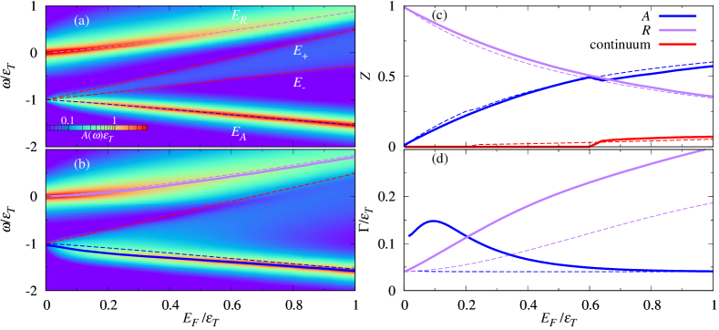
Numerous theoretical works have so far analyzed the zero-temperature properties of an impurity interacting with a free Fermi gas, in the context of both semiconductor heterostructures Suris (2003); Sidler et al. (2017); Efimkin and MacDonald (2017); Rana et al. (2020, 2021a, 2021b); Efimkin et al. (2021) and ultracold atomic gases Massignan et al. (2014); Scazza et al. (2022). The main polaron properties at are summarized in Fig. 1. In panel (a) we plot the doping and energy dependence of the spectral function. One observes that the optical absorption is dominated by two polaron quasiparticle resonances: the attractive polaron branch at lower energy and the repulsive polaron branch at higher energy . The energies are evaluated from the positions of the absorption peaks in Fig. 1. Here, both polaron branches are quasiparticles in the sense that satisfy the condition Fetter and Walecka (2003)
| (19) |
which coincides with a pole of the exciton Green’s function when the corresponding imaginary part of the self-energy becomes small. Note that the repulsive branch eventually stops satisfying this condition when Ngampruetikorn et al. (2012), and thus ceases to be a polaron quasiparticle. This large doping regime is not analyzed in this work.
In the limit of vanishing doping, the attractive branch energy recovers the trion energy , while the repulsive branch energy reduces to the exciton energy, . (We remind the reader that we measure energies with respect to that of the exciton at rest). However, differently from the trion, whose energy blueshifts with doping due to its interactions with the surrounding electrons [see Ref. Parish (2011) and Eq. (61)], the attractive polaron branch redshifts with doping. At the same time, the repulsive polaron branch blueshifts with doping. Thus, at zero temperature, as soon as doping is finite, the attractive and repulsive polaron quasiparticles are no longer the trion and the exciton, respectively, even if they recover the corresponding energies at low doping. Furthermore, within the single particle-hole-excitation ansatz (4), the effective mass of the attractive polaron Schmidt et al. (2012); Parish and Levinsen (2013) does not evolve into the trion mass at low doping.
As far as the coupling to light of the polaron branches is concerned, at very low doping the repulsive branch retains all the spectral weight and the attractive branch is dark, as is also the case for the trion. However, when doping increases, there is a transfer of oscillator strength from the repulsive to the attractive branch. This is shown in Fig. 1(c), where we plot the doping dependence of the spectral weights for each branch. At low doping , grows linearly with , which agrees with the doping dependence of the trion oscillator strength Glazov (2020).
There are also important differences between the attractive and repulsive polaron branches at zero temperature, even though they both satisfy Eq. (19) for values of doping up to . The attractive polaron is always a sharp resonance, with a Lorentzian broadening coinciding with the intrinsic broadening — see Fig. 1(d). By solving the eigenvalue problem (6) at zero temperature, one finds that the attractive branch energy coincides with the lowest eigenvalue energy, , which is separated from the energy of the excited states by a gap. By contrast, the repulsive branch does not correspond to a specific eigenstate; rather it is composed of a continuum of eigenstates with closely spaced eigenvalues, resulting in a polaron quasiparticle with finite lifetime. As a consequence, its broadening grows monotonically with and only coincides with at small doping — see Fig. 1(d).
In between the attractive and repulsive branches, one can observe in Fig. 1(a) a continuum of trion and Fermi-sea-hole states with a well-defined relative momentum in the variational function . The boundaries of this so-called trion-hole continuum can be evaluated from the energy of a trion (see Appendix C) plus a hole separately. If the hole has zero momentum , then, because of momentum conservation, the trion is also at zero momentum and the upper boundary of the trion-hole continuum is
| (20) |
Conversely, the energy of the trion-hole lower bound is
| (21) |
where both the hole and trion are at , with an arbitrary direction, and is the trion energy [which can be evaluated from Eq. (58)]. Thus, at zero temperature and finite doping, the attractive branch is separated from the trion-hole continuum by an energy gap. Note that, while this is a consequence of considering a single excitation of the medium, our results are consistent with those of diagrammatic quantum Monte Carlo Goulko et al. (2016) which demonstrated that there is a region of anomalously low spectral weight (a “dark continuum”) above the narrow attractive polaron branch. Furthermore, calculations that incorporate Coulomb interactions between charges also obtain a suppression of spectral weight of this continuum Rana et al. (2020).
IV.2 Finite temperature
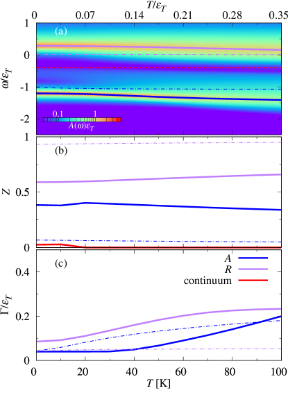
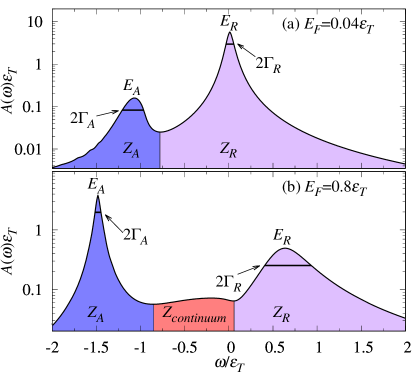
We now discuss the effect of temperature on the optical response. Figure 1(b-d) allows a comparison between the doping-dependent properties of optical absorption at zero and finite temperature. Both the energies and spectral weights of attractive and repulsive branches have a very weak dependence on temperature in the regime . The branch energies are slightly redshifted, while () is slightly smaller (larger) compared to the zero-temperature case. This small variation with temperature is also observed in Fig. 2(a,b) for a fixed doping. The most important difference at finite temperature is the behavior of the trion-hole continuum, which subsumes the attractive branch when , i.e., at sufficiently low doping or sufficiently high temperature. This can be clearly seen from Fig. 1(b), where we no longer observe a sharp lower bound of the trion-hole continuum at low doping because, at finite temperature, the unbound hole belonging to the trion-hole continuum can thermally occupy any momentum state. However, the upper bound of the trion-hole continuum is still clearly visible and approximately follows the zero-temperature expression (20). Similarly, for a fixed doping in Fig. 2(a), we observe that the trion-hole continuum is only well-separated from the attractive branch at low temperatures.
Since the spectral weight of the trion-hole continuum is small, its merging with the attractive branch only slightly affects the attractive peak energy. However, the disappearance of the attractive polaron quasiparticle strongly modifies the attractive-branch linewidth . In particular, we observe in Fig. 1(d) that has a striking non-monotonic dependence at low doping, while it decreases towards its zero-temperature value (corresponding to the intrinsic broadening ) when increases. Likewise, increasing the temperature at fixed doping can substantially increase from , as shown in Fig. 2(c). As we will discuss in Sec. IV.3, this behavior signals a crossover from a coherent Fermi polaron regime to an incoherent trion-dominated regime, where there no longer exists a well-defined attractive quasiparticle that is separated from the trion-hole continuum.
The repulsive branch, on the other hand, remains a polaron quasiparticle with a finite lifetime (broadening) for the dopings considered in this work (). In particular, we see that temperature does not change the nature of the repulsive branch in Figs. 1 and 2, but it can lead to a faster increase of the half linewidth with increasing doping [Fig. 1(d)].
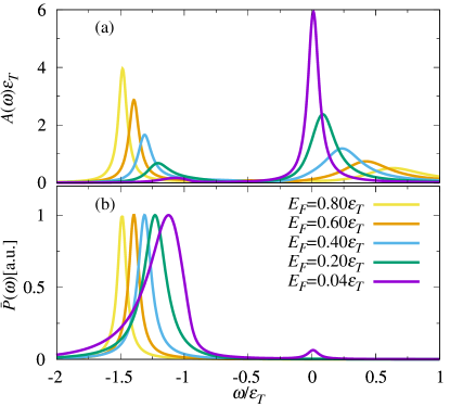
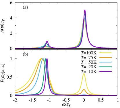
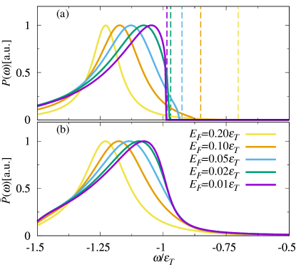
We now discuss the shape of the optical response profiles and how they evolve with either doping or temperature. Figures 3 and 4 display both the absorption and the Lorentzian convolved photoluminescence (see Appendix D) at fixed temperature and fixed doping, respectively. The repulsive polaron quasiparticle shows up approximately as a Lorentzian symmetric profile in both absorption and photoluminescence spectra, with a full width at half maximum (FWHM) that increases with increasing . Note that the FWHM of the repulsive branch only has a weak dependence on temperature in Fig. 4 since has been fixed to a low value such that the intrinsic width dominates [see Fig. 2(c)]. By contrast, the shape of the attractive branch is strongly modified by temperature: in the low-temperature (high-doping) regime , it is described by a Lorentzian with FWHM , while for , it develops a strongly asymmetric shape with an exponential tail below the trion energy. This evolution in the asymmetry of the attractive branch once again indicates a crossover from a Fermi-polaron quasiparticle to a continuum of trion states.
In Fig. 5 we further analyze the shape of the attractive peak at low doping , comparing the Lorentzian convolved photoluminescence with the “bare” photoluminescence , where we have removed the effects of any intrinsic exciton broadening. In panel (a), we observe a sharp onset of the photoluminescence which approximately coincides with the upper boundary of the trion-hole continuum at zero temperature, . Thus, according to Eq. (20), it blueshifts with increasing doping. As shown in Fig. 5(b), any intrinsic broadening only smooths out the sharp onset, while it has little effect on the position of the peak. When increases, the sharp onset tends to disappear as the attractive peak redshifts and detaches from the trion-hole continuum.
Our calculated profiles for the attractive branch are in excellent quantitative agreement with recent experiments in the high-temperature (low-doping) regime Zipfel et al. (2022), as discussed in the accompanying paper Mulkerin et al. (2022). The exponential tail of the asymmetric attractive peak has previously been modelled within a trion picture for the case of photoluminescence Esser et al. (2000, 2001); Ross et al. (2013); Christopher et al. (2017). There, the tail is ascribed to the kinetic energy of remaining electrons after the exciton within each trion has decayed into a photon. This description in terms of electron recoil can be formally derived from our theory in the limit of weak interactions, as we will discuss in Sec. IV.4.
IV.3 Loss of the attractive polaron quasiparticle: polaron to trion-hole continuum crossover
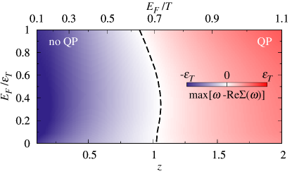
In this section, we use the pole condition in Eq. (19) to characterize the crossover from a well-defined polaron quasiparticle to a trion-hole continuum with increasing temperature (decreasing doping). In order to find the values of temperature and doping at which this crossover occurs, we plot in Fig. 6 the local maximum value of the function for and identify the curve of doping versus fugacity at which this maximum value is zero. For , we find that this occurs roughly when and thus . On the left of this curve, we lose the attractive polaron quasiparticle, as the condition (19) cannot be satisfied, i.e., . On the right of this curve, instead, the system is in the polaron regime where (19) is satisfied.
In order to further illustrate this crossover, we compare the results for the polaron energies, spectral weights and linewidths extracted from the spectral function with those obtained by treating the polaron as a well-defined quasiparticle Fetter and Walecka (2003). In the latter case, the polaron properties can be obtained directly from the expression of the impurity self-energy. Close to a quasiparticle resonance, the exciton Green’s function can be approximated as
| (22) |
where is the two-branch index, and the quasiparticle energy is a solution of Eq. (19). The pole weight or residue is
| (23) |
and the polaron damping rate is
| (24) |
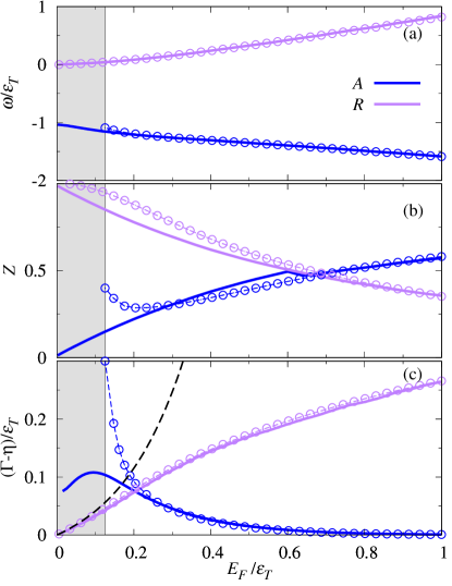
We compare the results for , , and obtained with both methods in Fig. 7. We observe that the positions of the poles coincide to high accuracy with those of the spectral function maxima — see panel (a). For the repulsive branch, both the spectral weight and the broadening from the quasiparticle theory are in good agreement with those evaluated from the spectral function, even when the linewidth is non-negligible. By contrast, for the attractive branch, the results depart from one another when we approach the (gray) region where there is no attractive quasiparticle, and the quasiparticle description breaks down since, according to Eq. (23), when .
In the following section, we analyze the system properties well inside the trion-hole continuum (gray) regime, where the attractive branch is no longer a polaron quasiparticle. Here, for temperatures , we can apply a systematic quantum virial expansion. This connects the results of this work with those obtained in the accompanying paper Mulkerin et al. (2022).
IV.4 Virial expansion and connection to the trion wave function at high temperature or low doping
As discussed, at high temperature or low doping such that the fugacity , the attractive polaron quasiparticle disappears and the attractive branch only consists of a broad continuum. In this limit, one can formally apply a perturbatively exact quantum virial expansion in the fugacity Mulkerin et al. (2022). We will now briefly discuss how this expansion is related to the polaron theory, and how this allows us to demonstrate that the trion picture results of Refs. Esser et al. (2000); Zipfel et al. (2022) are contained within the polaron formalism.
When and , we can formally expand the Fermi occupation function which then coincides with the Boltzmann distribution . Likewise, to leading order in we have — see Eq. (12). Within this expansion, the exciton self-energy in Eq. (10) becomes
| (25) |
In other words, to leading order in the fugacity, the self-energy is determined by two-body interactions weighted by a Boltzmann distribution.
Focusing first on the attractive branch, the dominant contribution to the self-energy arises from the pole of the matrix at the trion energy. We therefore expand the matrix for , with the result
| (26) |
where . The matrix can be expressed in terms of the vacuum () trion wave function for a contact electron-exciton interaction (see Appendix F). In our case, the relative momentum is , and therefore the kinetic energy of the relative motion is . Using the expression for the vacuum trion wave function in the center of mass frame, (see Appendix C), we have
| (27) |
Here, the numerator is derived by manipulating the relation between the trion wave function and , and is momentum independent. However, this is a special property of the contact electron-exciton interaction, and Eq. (27) in fact yields the correct generalization for an arbitrary electron-exciton interaction that leads to the formation of a trion. In other words, it can be applied for any realistic trion wave function. For details of the generalization to arbitrary interactions, see Appendix F.
Using the approximation for the vacuum matrix, Eq. (27), the self-energy in Eq. (25) becomes
| (28) |
where denotes the principal value. This explicitly relates the self-energy calculated within the polaron theory to the trion wave function in the regime where the fugacity is small, and importantly it applies for any realistic trion wave function. A similar approach involving trion wave functions has been used to calculate absorption Bronold (2000). Note that the real part diverges logarithmically when , and therefore it cannot in general be neglected close to the onset of the attractive branch.
For the repulsive branch, we can again apply Eq. (25) to find the leading contribution at small fugacity. In the regime where , the width of the repulsive branch is much smaller than the trion binding energy, and to lowest order in the fugacity, we can simply evaluate the repulsive polaron self-energy within the repulsive branch by taking . We then use the fact that, to logarithmic accuracy, the logarithmic behavior at small momentum is generic for the vacuum matrix for any short-range interaction Adhikari (1986); Landau and Lifshitz (2013) and thus we have
| (29) |
where is the Euler-Mascheroni constant. Here, we have evaluated the integral by noting that the integral is dominated by for small , and the inclusion of originates from expanding the integral to the first subleading order in .
The self-energies in Eqs. (28) and (29) can now be directly inserted into the Dyson equation (9) to yield the absorption in Eq. (13) or the photoluminescence in Eq. (18). To be explicit, within the virial expansion we have the exciton spectral function
| (30) |
This yields a broad continuum for the attractive branch, where the spectral weight vanishes at , and when we are far below this onset, we have . Therefore we have an exponential tail modulated by the trion wave function:
| (31) |
The peak of the absorption is between the onset and the tail, and therefore it will not correspond to the vacuum trion energy. This can lead to an overestimate of the trion binding energy in experiments Zipfel et al. (2022), as shown in the accompanying paper Mulkerin et al. (2022). From Eq. (29), we find that the repulsive branch is a Lorentzian of width . We have compared in Fig. 7(c) this expression against the numerical evaluation of the repulsive branch half linewidth (where we have removed the effect of the intrinsic exciton lifetime), finding excellent agreement at low doping, inside the region of validity of the virial expansion.
For the photoluminescence, we find
| (32) |
where we have used the fact that the width of the repulsive branch is much smaller than the temperature, and thus the repulsive branch is very weakly modified by the Boltzmann factor.
IV.5 Connection to the trion theory of electron recoil
Finally, we discuss how our theory relates to the calculation of electron recoil in previous trion-picture calculations such as by Esser et al., Refs. Esser et al. (2000, 2001). As we shall demonstrate, that theory corresponds to a weak-interaction limit of the low doping/high temperature version of our polaron theory. To see this, we take the limit of a small self-energy in the Dyson equation in Eq. (9) as follows:
| (33) |
Since the terms only have a pole at (i.e., at the bare exciton energy), the attractive branch is obtained from the imaginary part of the self-energy. The detailed balance equation (18) then implies that the corresponding PL from the attractive branch is
| (34) |
where we used Eq. (28). Up to frequency-independent prefactors, this precisely matches the result of Esser et al. Thus, the trion-picture PL is already contained within the polaron picture. However, as we have already argued, the trion picture calculation assumes that we are in a weakly interacting limit where the self-energy is much smaller than the frequency. This assumption manifestly breaks down close to the onset of the attractive branch, where the real part of the self-energy diverges, and hence the previous trion picture calculation fails to correctly describe the onset and shape of the attractive branch. On the other hand, it correctly identifies the exponential tail of the PL, which is dominated by the imaginary part of the self-energy.
For the repulsive branch, the trion picture again uses the weak-interaction limit of the Dyson equation (33), this time neglecting even the second term on the right hand side. This results in
| (35) |
with a small correction that counteracts the oscillator strength transferred to the attractive branch Esser et al. (2001). We see that the trion picture fails to describe the Lorentzian shape of the repulsive polaron, which arises from the exciton-electron scattering states as well as the full Dyson series.
V Strong light-matter coupling
We now extend the formalism of Sec. III to describe recent experiments where a doped TMD monolayer was embedded into a microcavity Sidler et al. (2017); Chakraborty et al. (2018); Emmanuele et al. (2020); Koksal et al. (2021); Lyons et al. (2022). In this case, the strong coupling between light and matter can lead to the formation of Fermi polaron-polaritons Baeten and Wouters (2015); Sidler et al. (2017). A particularly important question is whether there still exists strong coupling to light either because of temperature induced broadening effects or because the attractive branch does not correspond to a well-defined quasiparticle.
To describe the light-matter coupled system, we add two terms describing cavity photons and the photon-exciton interaction to the Hamiltonian (1):
| (36a) | ||||
| (36b) | ||||
| (36c) | ||||
Photons are described by the bosonic creation operator and, in a cavity, they acquire a quadratic dispersion Kavokin et al. (2017), where is the photon-exciton energy detuning. Typically the photon mass in a planar microcavity is Kavokin et al. (2017). The term (36c) describes an exciton recombining to emit a photon and vice versa, with a coupling strength given by the Rabi splitting Kavokin et al. (2017). In monolayer TMDs, this is typically in the range of 1-2 Liu et al. (2014); Dufferwiel et al. (2015).
In order to derive the photon Green’s function and the optical absorption in the strong coupling regime, one can follow the same procedure employed in Sec. III. The difference is that now we formulate a variational ansatz for the time-dependent photon operator, with an analogous form to (4):
| (37) |
We neglect the dressing of the photon operator by a particle-hole excitation . This term involves photon recoil, and therefore implies energies far off resonance from the exciton and trion energies because of the extremely small mass of the photon.
To obtain the eigenvalue problem for the light-matter coupled system, we introduce the error operator corresponding to the photon and minimize the error function, Eq. (5), with respect to the variational coefficients , , and . Considering the stationary solutions, we find
| (38a) | ||||
| (38b) | ||||
| (38c) | ||||
where we have again neglected terms that vanish in the limit These equations reduce to those for the exciton polaron, Eq. (6), when we take and . By following an analogous derivation to that in Sec. III, one can easily demonstrate that the retarded photon Green’s function in the frequency domain is given by:
| (39) |
For the same reason that we can neglect the particle-hole dressing of the photon operator in the ansatz (37), the expressions for the exciton self-energy in Eqs. (10) and (11) are not affected by the coupling to light. Therefore, we can derive the coupled exciton and photon Green’s functions in the strong coupling regime by inverting the matrix Levinsen et al. (2019)
and evaluating the diagonal elements, giving:
| (40a) | ||||
| (40b) | ||||
The expression (40a) for the exciton Green’s function in terms of the self-energy can also be obtained by following the same procedure as in Appendix B, where we have first eliminated the photon amplitude by solving Eq. (38c), i.e., . Finally, in the strong coupling regime, optical absorption coincides (up to a frequency-independent prefactor) with the photon spectral function Ćwik et al. (2016):
| (41) |
which we will focus on in the following.
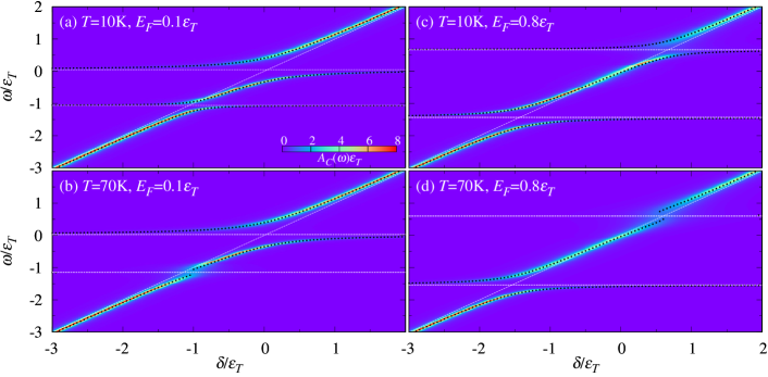
We plot in Fig. 8 the finite-temperature photon spectral function at normal incidence as a function of energy and detuning . When , the strong coupling to light leads to three polariton branches, the lower (LP), middle (MP), and upper polariton (UP), as can be seen in Fig. 8(a,c).
The existence of these polariton modes is connected to the attractive and repulsive exciton branches in the presence of doping. We can capture the behavior of the Fermi polaron-polaritons by employing a three coupled oscillator model, which yields the following simplified expression for the photon Green’s function
| (42) | ||||
| (43) |
Here, we have explicitly included a cavity photon lifetime and we have used the extracted parameters for the exciton-polaron branches in the absence of coupling to light, namely the energies , spectral weights , and half linewidths . Note that we cannot evaluate the polariton branch energies as the (complex) eigenvalues of the matrix Savona et al. (1995). Rather, we have to evaluate first the photon spectral function (41) and then determine the polariton energies from the photon spectral function peak positions. The comparison in Fig. 8 between the LP, MP and UP energies obtained in this way and the full calculation demonstrates essentially perfect agreement.
Remarkably, we find that a strong enough light-matter coupling can produce well-defined polariton quasiparticles (where ) for the lower and middle branches even when there is no attractive polaron quasiparticle and Eq. (19) is not satisfied. However, once the linewidths approach , the energy splitting between branches closes, indicating a loss of strong coupling. We observe this in the low-doping regime for LP and MP [Fig. 8(b)], and in the high-doping regime for MP and UP [Fig. 8(c,d)]. Within the three coupled oscillator model, this transition from weak to strong light-matter coupling approximately occurs when , as expected, though there are small deviations when the attractive branch is no longer a well-defined polaron quasiparticle. To conclude, the effect of temperature on this transition can be easily accounted for by considering its effect on the quasiparticle linewidths and spectral weights (see Sec. IV).
VI Conclusions and perspectives
We have studied the optical properties of a doped two-dimensional semiconductor at a finite temperature using a Fermi-polaron approach involving a single excitation of the fermionic medium. Our results reveal that the attractive branch can experience a smooth transition from a regime where it is a well-defined quasiparticle to a regime where is subsumed into a broad continuum of trion-hole scattering states. This crossover results in a strong change in the spectral lineshape and can be driven by either decreasing doping or increasing temperature, but it cannot occur at zero temperature. While the Fermi polaron theory is able to capture both limits, theories based on the trion wavefunction necessarily only apply in the limit where there is no a well-defined quasiparticle. In particular, we formally show that the trion theory corresponds to a weak-interaction limit of our finite-temperature Fermi polaron theory.
In the regime of strong light-matter coupling, we have shown how the temperature can modify the properties of the Fermi polaron-polaritons. We demonstrate that the strong-to-weak coupling crossover observed at finite temperature for the attractive branch at low enough doping and the repulsive branch in the high doping regime can be explained in terms of the linewidths and spectral weights of the two branches.
In future studies, it would be interesting to investigate how the quasiparticle transition of the attractive branch, driven by either temperature or doping, would affect the interactions between exciton impurities. In particular, common descriptions of polaron-polaron interactions use Landau’s theory of dilute solutions Yu and Pethick (2012), which assumes well-defined quasiparticles. Such interactions could, for instance, be measured using coherent multidimensional spectroscopy on gated 2D materials, similarly to recent experiments on intrinsically doped samples Muir et al. (2022).
Acknowledgements.
We gratefully acknowledge useful discussions with Dmitry Efimkin. AT and FMM acknowledge financial support from the Ministerio de Ciencia e Innovación (MICINN), project No. AEI/10.13039/501100011033 (2DEnLight). FMM acknowledges financial support from the Proyecto Sinérgico CAM 2020 Y2020/TCS-6545 (NanoQuCo-CM). JL and MMP are supported through Australian Research Council Future Fellowships FT160100244 and FT200100619, respectively. JL, BM and MMP also acknowledge support from the Australian Research Council Centre of Excellence in Future Low-Energy Electronics Technologies (CE170100039).Appendix A Finite impurity momentum
For completeness, we generalize the finite-temperature polaron formalism illustrated in Sec. III to absorption and photoluminescence at finite momentum. This can in principle be measured in doped semiconductors using angle-resolved photoemission spectroscopy Madéo et al. (2020); Man et al. (2021). Similarly to Eq. (4), we approximate the exciton operator in the Heisenberg picture at finite momentum as
| (44) |
The derivation then follows similarly to the zero momentum case. We minimize the error function , where , obtaining the following eigenvalue problem:
| (45a) | ||||
| (45b) | ||||
where . The exciton Green’s function can thus be written in terms of the eigenvalues and eigenvectors as
| (46) |
Equivalently, the exciton Green’s function can be written in terms of the exciton self-energy at finite momentum
| (47) | ||||
| (48) |
where the inverse of the matrix is defined in Eq. (11). This follows the same procedure as in the case of , which is described in Appendix B.
The absorption of a photon with momentum is given by
| (49) |
Absorption and photoluminescence can be connected using detailed balance conditions as derived in the main text, starting from the Fermi’s golden rule definitions:
| (50a) | ||||
| (50b) | ||||
Thus, the detailed balance condition is identical to that at zero momentum:
| (51) |
Appendix B Exciton self-energy
In this appendix, we demonstrate that the exciton self-energy can be derived starting from the eigenvalue equations (6) and that it coincides with the expression (10) that can be derived within a matrix formalism. Let us start from the eigenvalue problem (6) which can be rewritten in terms of the auxiliary function :
| (52a) | ||||
| (52b) | ||||
| (52c) | ||||
Introducing Eq. (52c) into Eq. (52a) and solving for we obtain
| (53) |
where we have used that in the limit . Substituting (53) into Eq. (52b), one thus finally obtains an implicit equation for the energy :
| (54) |
This expression coincides with the pole of the exciton Green’s function (9) and therefore we can identify the self-energy term correcting the exciton energy because of the exciton-electron interaction as the term:
| (55) |
Recalling that , we obtain exactly the expression (10) in the main text. By a completely equivalent procedure, we can arrive at the self-energy in the case of finite exciton momentum, Eq. (48).
Appendix C Trion
In this appendix, we summarize for completeness the known trion properties within our model Hamiltonian (1). At zero temperature, a trion with momentum in the presence of a Fermi sea is described as:
| (56) |
The trion wave function satisfies the Schrödinger equation Parish (2011)
| (57) |
and the trion energy can be evaluated by solving the implicit equation:
| (58) |
Note that some care has to be taken when comparing the trion energy with that of a bare exciton, since the Fermi sea in Eq. (56) involves one less electron. This difference has been taken into account in Eqs. (20) and (21) of the main text. We now discuss the solution of Eq. (58) in various limits.
When , it is profitable to introduce the relative momentum in the center of mass frame , so that the electron momentum becomes , with , where is the trion mass, and the exciton momentum becomes , with . Now one has that relative and center of mass kinetic energies factorize, , where , is the trion reduced mass, and . Thus, the trion energy and wave function are given by
| (59) | ||||
| (60) |
where and where .
At finite doping and zero momentum , Eqs. (57) and (58) can also be solved exactly to give
| (61) | ||||
| (62) |
At finite doping and finite momentum, Eq. (58) can be solved analytically Parish and Levinsen (2013) to find an implicit equation for . Here, one finds that the trion acquires a finite momentum when .
We can now analyze the trion coupling strength to light. At zero doping, , trions do not couple to light, and thus cannot be probed optically. This is because the matrix element between a trion state and a cavity photon plus a majority particle at zero momentum of the light-matter interaction term is given by
| (63) |
Taking the squared amplitude of this matrix element, we see that the coupling to light of a single trion scales as , which is vanishingly small.
On the other hand, if we have electrons within , then the coupling to light scales instead as . Thus, even though the coupling per electron vanishes, the net effect of having an electronic medium is to create a continuum of states, with a total spectral weight that scales as , in agreement with Ref. Glazov (2020).
Appendix D Numerical evaluation of the many-body matrix and the exciton self-energy
In contrast to the vacuum matrix (12b), the many-body correction in Eq. (12c) cannot be evaluated analytically. The approach we illustrate in the following allows us to treat it in a simpler way and to evaluate it numerically, even when the intrinsic exciton linewidth is set to zero. Let us start by re-writing (12c) in an equivalent form:
| (64) |
The -integral can then be evaluated numerically by applying the Sokhotski–Plemelj theorem
where is the integral principal part.
As far as the -integral for evaluating the exciton self-energy (10) is concerned, it can be re-written in the following equivalent form by defining :
This integral has a pole when . Using a model involving contact interactions in 2D means that such a pole always exists, and furthermore it is a simple pole Engelbrecht and Randeria (1992). Thus, we define to be the pole of the matrix.
In this case, we can apply the Cauchy residue theorem to write:
| (65) |
where the principal part prescription is used in the vicinity of the pole at , and the residue can be evaluated as
| (66) |
From the expression of the exciton self-energy, we can get the exciton Green’s function (9), absorption (13), and photoluminesence (18). These results allow us to evaluate the absorption and photoluminescence without any intrinsic homogeneous broadening for the exciton. For absorption alone, the integration method illustrated here is unnecessary, as one can conveniently shift the frequency to the complex plane, , where is related to the exciton decay rate, giving well converged results. However, as explained in the main text, for the luminescence one has to adopt the numerical method illustrated here. Thus, in order to compare with experiments, we introduce the effect of lifetime broadening at the end by convolving the photoluminescence with a Lorentzian profile with broadening :
| (67) |
Appendix E Extracting polaron properties at finite temperature
In this appendix we illustrate how to extract the polaron energies, spectral weights, and half linewidths of Figs. 1 and 2 from the spectral function profile . This is illustrated in Fig. 9. The polaron energy is evaluated as the spectral function peak position, the linewidth as the full width at half maximum (FWHM) and the spectral weight as the area under the peak. We have used the location of the spectral function minima as limits for the integrals evaluating the spectral weights: If there is only one minimum, this is the upper (lower) bound for evaluating (), while if there are two minima, these are the limits for evaluating the trion-hole continuum spectral weight . This criterion is the origin of the discontinuity of the residues in Figs. 1, 2, and 7.
Note that, in the cases shown in Fig. 9, at low doping of panel (a) the trion-hole continuum does not appear because is merged with the attractive branch, which in this case, ceases to be a polaron quasiparticle resonance in the sense explained in Sec. IV.3. This can also be appreciated by the non-Lorentzian and asymmetric form of the spectral function around . By contrast, at larger doping in panel (b), the attractive branch is separated from the continuum, is a polaron quasiparticle in this case and recovers the Lorentzian symmetric shape.
Appendix F Relationship between electron-exciton matrix and the trion wave function
While Eq. (28) was derived for the special case of contact exciton-electron interactions, it is in fact general and can be applied for any realistic trion wave function. To see this, we note that the generalization of Eq. (25) to arbitrary two-body transition operator is
| (68) |
We have defined the two-body state in terms of the relative momentum and the total momentum which are related to the electron momentum via and the exciton momentum via .
To evaluate the matrix element of the transition operator for an electron-exciton interaction that yields a trion bound state, we use the relationship between the Green’s operator and the transition operator at energy :
| (69) |
Here, and (which, for the two-body problem, should be evaluated in the canonical ensemble, effectively taking ). Close to the trion resonance, we can neglect the first term, and we therefore have the spectral representation
| (70) |
where in the third step we approximated the expectation value by inserting the trion state, and in the last step we used the pole condition. Taking and using we see that Eq. (68) reduces to Eq. (28) which demonstrates that it holds for arbitrary electron-exciton interactions that lead to trion formation.
In the special case of contact interactions, the numerator of Eq. (F) reduces to due to Eq. (60), and therefore it reproduces the pole expansion in Eq. (26) as it should. Note that the fact that the matrix in this case is independent of the relative momentum is a special feature of contact interactions.
References
- Landau (1933) L. D. Landau, Über die Bewegung der Elektronen in Kristalgitter, Phys. Z. Sowjetunion 3, 644 (1933).
- Massignan et al. (2014) P. Massignan, M. Zaccanti, and G. M. Bruun, Polarons, dressed molecules and itinerant ferromagnetism in ultracold Fermi gases, Reports on Progress in Physics 77, 034401 (2014).
- Levinsen and Parish (2015) J. Levinsen and M. M. Parish, Strongly interacting two-dimensional Fermi gases, Annual Review of Cold Atoms and Molecules 3, 1 (2015).
- Scazza et al. (2022) F. Scazza, M. Zaccanti, P. Massignan, M. M. Parish, and J. Levinsen, Repulsive Fermi and Bose Polarons in Quantum Gases, Atoms 10 (2022).
- Bardeen et al. (1967) J. Bardeen, G. Baym, and D. Pines, Effective Interaction of 3He Atoms in Dilute Solutions of 3He in 4He at Low Temperatures, Phys. Rev. 156, 207 (1967).
- Kondo (1964) J. Kondo, Resistance Minimum in Dilute Magnetic Alloys, Progress of Theoretical Physics 32, 37 (1964).
- Sidler et al. (2017) M. Sidler, P. Back, O. Cotlet, A. Srivastava, T. Fink, M. Kroner, E. Demler, and A. Imamoglu, Fermi polaron-polaritons in charge-tunable atomically thin semiconductors, Nature Physics 13, 255 (2017).
- Goldstein et al. (2020) T. Goldstein, Y.-C. Wu, S.-Y. Chen, T. Taniguchi, K. Watanabe, K. Varga, and J. Yan, Ground and excited state exciton polarons in monolayer MoSe2, The Journal of Chemical Physics 153, 071101 (2020).
- Koksal et al. (2021) O. Koksal, M. Jung, C. Manolatou, A. N. Vamivakas, G. Shvets, and F. Rana, Structure and dispersion of exciton-trion-polaritons in two-dimensional materials: Experiments and theory, Phys. Rev. Research 3, 033064 (2021).
- Liu et al. (2021) E. Liu, J. van Baren, Z. Lu, T. Taniguchi, K. Watanabe, D. Smirnov, Y.-C. Chang, and C. H. Lui, Exciton-polaron Rydberg states in monolayer MoSe2 and WSe2, Nature Communications 12, 6131 (2021).
- Xiao et al. (2021) K. Xiao, T. Yan, Q. Liu, S. Yang, C. Kan, R. Duan, Z. Liu, and X. Cui, Many-Body Effect on Optical Properties of Monolayer Molybdenum Diselenide, The Journal of Physical Chemistry Letters 12, 2555 (2021).
- Zipfel et al. (2022) J. Zipfel, K. Wagner, M. A. Semina, J. D. Ziegler, T. Taniguchi, K. Watanabe, M. M. Glazov, and A. Chernikov, Electron recoil effect in electrically tunable monolayers, Phys. Rev. B 105, 075311 (2022).
- Suris (2003) R. A. Suris, Correlation Between Trion and Hole in Fermi Distribution in Process of Trion Photo-Excitation in Doped QWs, in Optical Properties of 2D Systems with Interacting Electrons (Springer Netherlands, 2003) pp. 111–124.
- Efimkin and MacDonald (2017) D. K. Efimkin and A. H. MacDonald, Many-body theory of trion absorption features in two-dimensional semiconductors, Phys. Rev. B 95, 035417 (2017).
- Rana et al. (2020) F. Rana, O. Koksal, and C. Manolatou, Many-body theory of the optical conductivity of excitons and trions in two-dimensional materials, Phys. Rev. B 102, 085304 (2020).
- Rana et al. (2021a) F. Rana, O. Koksal, M. Jung, G. Shvets, and C. Manolatou, Many-body theory of radiative lifetimes of exciton-trion superposition states in doped two-dimensional materials, Phys. Rev. B 103, 035424 (2021a).
- Rana et al. (2021b) F. Rana, O. Koksal, M. Jung, G. Shvets, A. N. Vamivakas, and C. Manolatou, Exciton-Trion Polaritons in Doped Two-Dimensional Semiconductors, Phys. Rev. Lett. 126, 127402 (2021b).
- Efimkin et al. (2021) D. K. Efimkin, E. K. Laird, J. Levinsen, M. M. Parish, and A. H. MacDonald, Electron-exciton interactions in the exciton-polaron problem, Phys. Rev. B 103, 075417 (2021).
- Chakraborty et al. (2018) B. Chakraborty, J. Gu, Z. Sun, M. Khatoniar, R. Bushati, A. L. Boehmke, R. Koots, and V. M. Menon, Control of Strong Light–Matter Interaction in Monolayer WS2 through Electric Field Gating, Nano Letters 18, 6455 (2018), pMID: 30160968.
- Emmanuele et al. (2020) R. P. A. Emmanuele, M. Sich, O. Kyriienko, V. Shahnazaryan, F. Withers, A. Catanzaro, P. M. Walker, F. A. Benimetskiy, M. S. Skolnick, A. I. Tartakovskii, I. A. Shelykh, and D. N. Krizhanovskii, Highly nonlinear trion-polaritons in a monolayer semiconductor, Nature Communications 11, 3589 (2020).
- Lyons et al. (2022) T. P. Lyons, D. J. Gillard, C. Leblanc, J. Puebla, D. D. Solnyshkov, L. Klompmaker, I. A. Akimov, C. Louca, P. Muduli, A. Genco, M. Bayer, Y. Otani, G. Malpuech, and A. I. Tartakovskii, Giant effective Zeeman splitting in a monolayer semiconductor realized by spin-selective strong light–matter coupling, Nature Photonics 16, 632 (2022).
- Tan et al. (2020) L. B. Tan, O. Cotlet, A. Bergschneider, R. Schmidt, P. Back, Y. Shimazaki, M. Kroner, and A. İmamoğlu, Interacting Polaron-Polaritons, Phys. Rev. X 10, 021011 (2020).
- Kyriienko et al. (2020) O. Kyriienko, D. N. Krizhanovskii, and I. A. Shelykh, Nonlinear Quantum Optics with Trion Polaritons in 2D Monolayers: Conventional and Unconventional Photon Blockade, Phys. Rev. Lett. 125, 197402 (2020).
- Efimkin and MacDonald (2018) D. K. Efimkin and A. H. MacDonald, Exciton-polarons in doped semiconductors in a strong magnetic field, Phys. Rev. B 97, 235432 (2018).
- Cotleţ et al. (2019) O. Cotleţ, F. Pientka, R. Schmidt, G. Zarand, E. Demler, and A. Imamoglu, Transport of Neutral Optical Excitations Using Electric Fields, Phys. Rev. X 9, 041019 (2019).
- Smoleński et al. (2019) T. Smoleński, O. Cotlet, A. Popert, P. Back, Y. Shimazaki, P. Knüppel, N. Dietler, T. Taniguchi, K. Watanabe, M. Kroner, and A. Imamoglu, Interaction-Induced Shubnikov–de Haas Oscillations in Optical Conductivity of Monolayer , Phys. Rev. Lett. 123, 097403 (2019).
- Chervy et al. (2020) T. Chervy, P. Knüppel, H. Abbaspour, M. Lupatini, S. Fält, W. Wegscheider, M. Kroner, and A. Imamoǧlu, Accelerating Polaritons with External Electric and Magnetic Fields, Phys. Rev. X 10, 011040 (2020).
- Smoleński et al. (2021) T. Smoleński, P. E. Dolgirev, C. Kuhlenkamp, A. Popert, Y. Shimazaki, P. Back, X. Lu, M. Kroner, K. Watanabe, T. Taniguchi, I. Esterlis, E. Demler, and A. Imamoğlu, Signatures of Wigner crystal of electrons in a monolayer semiconductor, Nature 595, 53 (2021).
- Shimazaki et al. (2021) Y. Shimazaki, C. Kuhlenkamp, I. Schwartz, T. Smoleński, K. Watanabe, T. Taniguchi, M. Kroner, R. Schmidt, M. Knap, and A. m. c. Imamoğlu, Optical Signatures of Periodic Charge Distribution in a Mott-like Correlated Insulator State, Phys. Rev. X 11, 021027 (2021).
- Popert et al. (2022) A. Popert, Y. Shimazaki, M. Kroner, K. Watanabe, T. Taniguchi, A. Imamoğlu, and T. Smoleński, Optical Sensing of Fractional Quantum Hall Effect in Graphene, Nano Letters 22, 7363 (2022), pMID: 36124418.
- Schwartz et al. (2021) I. Schwartz, Y. Shimazaki, C. Kuhlenkamp, K. Watanabe, T. Taniguchi, M. Kroner, and A. Imamoğlu, Electrically tunable Feshbach resonances in twisted bilayer semiconductors, Science 374, 336 (2021).
- Note (1) While the results in Refs. Baeten and Wouters (2015); Rana et al. (2020) have been derived at finite temperature, the former only considered infinite exciton mass, while the latter did not analyze the consequences of temperature on the polaron description.
- Yan et al. (2019) Z. Yan, P. B. Patel, B. Mukherjee, R. J. Fletcher, J. Struck, and M. W. Zwierlein, Boiling a Unitary Fermi Liquid, Phys. Rev. Lett. 122, 093401 (2019).
- Bronold (2000) F. Bronold, Absorption spectrum of a weakly n-doped semiconductor quantum well, Phys. Rev. B 61, 12620 (2000).
- Carbone et al. (2020) M. R. Carbone, M. Z. Mayers, and D. R. Reichman, Microscopic model of the doping dependence of linewidths in monolayer transition metal dichalcogenides, The Journal of Chemical Physics 152, 194705 (2020).
- Zhumagulov et al. (2020) Y. V. Zhumagulov, A. Vagov, D. R. Gulevich, P. E. Faria Junior, and V. Perebeinos, Trion induced photoluminescence of a doped MoS2 monolayer, The Journal of Chemical Physics 153, 044132 (2020).
- Liu et al. (2019) W. E. Liu, J. Levinsen, and M. M. Parish, Variational Approach for Impurity Dynamics at Finite Temperature, Phys. Rev. Lett. 122, 205301 (2019).
- Mulkerin et al. (2022) B. C. Mulkerin, A. Tiene, F. M. Marchetti, M. M. Parish, and J. Levinsen, Virial expansion for the optical response of doped two-dimensional semiconductors (2022), accompanying paper.
- Koschorreck et al. (2012) M. Koschorreck, D. Pertot, E. Vogt, B. Fröhlich, M. Feld, and M. Köhl, Attractive and repulsive Fermi polarons in two dimensions, Nature 485, 619 (2012).
- Zhang et al. (2012) Y. Zhang, W. Ong, I. Arakelyan, and J. E. Thomas, Polaron-to-Polaron Transitions in the Radio-Frequency Spectrum of a Quasi-Two-Dimensional Fermi Gas, Phys. Rev. Lett. 108, 235302 (2012).
- Darkwah Oppong et al. (2019) N. Darkwah Oppong, L. Riegger, O. Bettermann, M. Höfer, J. Levinsen, M. M. Parish, I. Bloch, and S. Fölling, Observation of Coherent Multiorbital Polarons in a Two-Dimensional Fermi Gas, Phys. Rev. Lett. 122, 193604 (2019).
- Tiene et al. (2022) A. Tiene, J. Levinsen, J. Keeling, M. M. Parish, and F. M. Marchetti, Effect of fermion indistinguishability on optical absorption of doped two-dimensional semiconductors, Phys. Rev. B 105, 125404 (2022).
- Glazov (2020) M. M. Glazov, Optical properties of charged excitons in two-dimensional semiconductors, The Journal of Chemical Physics 153, 034703 (2020).
- Fey et al. (2020) C. Fey, P. Schmelcher, A. Imamoglu, and R. Schmidt, Theory of exciton-electron scattering in atomically thin semiconductors, Phys. Rev. B 101, 195417 (2020).
- Kormányos et al. (2015) A. Kormányos, G. Burkard, M. Gmitra, J. Fabian, V. Zólyomi, N. D. Drummond, and V. Fal’ko, kp theory for two-dimensional transition metal dichalcogenide semiconductors, 2D Materials 2, 022001 (2015).
- Cetina et al. (2016) M. Cetina, M. Jag, R. S. Lous, I. Fritsche, J. T. M. Walraven, R. Grimm, J. Levinsen, M. M. Parish, R. Schmidt, M. Knap, and E. Demler, Ultrafast many-body interferometry of impurities coupled to a Fermi sea, Science 354, 96 (2016).
- Scazza et al. (2017) F. Scazza, G. Valtolina, P. Massignan, A. Recati, A. Amico, A. Burchianti, C. Fort, M. Inguscio, M. Zaccanti, and G. Roati, Repulsive Fermi Polarons in a Resonant Mixture of Ultracold 6Li Atoms, Phys. Rev. Lett. 118, 083602 (2017).
- Adlong et al. (2020) H. S. Adlong, W. E. Liu, F. Scazza, M. Zaccanti, N. D. Oppong, S. Fölling, M. M. Parish, and J. Levinsen, Quasiparticle Lifetime of the Repulsive Fermi Polaron, Phys. Rev. Lett. 125, 133401 (2020).
- Liu et al. (2020a) W. E. Liu, Z.-Y. Shi, J. Levinsen, and M. M. Parish, Radio-Frequency Response and Contact of Impurities in a Quantum Gas, Phys. Rev. Lett. 125, 065301 (2020a).
- Chevy (2006) F. Chevy, Universal phase diagram of a strongly interacting Fermi gas with unbalanced spin populations, Phys. Rev. A 74, 063628 (2006).
- Combescot et al. (2007) R. Combescot, A. Recati, C. Lobo, and F. Chevy, Normal State of Highly Polarized Fermi Gases: Simple Many-Body Approaches, Phys. Rev. Lett. 98, 180402 (2007).
- Liu et al. (2020b) W. E. Liu, Z.-Y. Shi, M. M. Parish, and J. Levinsen, Theory of radio-frequency spectroscopy of impurities in quantum gases, Phys. Rev. A 102, 023304 (2020b).
- Kubo (1957) R. Kubo, Statistical-Mechanical Theory of Irreversible Processes. I. General Theory and Simple Applications to Magnetic and Conduction Problems, Journal of the Physical Society of Japan 12, 570 (1957).
- Martin and Schwinger (1959) P. C. Martin and J. Schwinger, Theory of Many-Particle Systems. I, Phys. Rev. 115, 1342 (1959).
- Kennard (1918) E. H. Kennard, On The Thermodynamics of Fluorescence, Phys. Rev. 11, 29 (1918).
- Stepanov (1957) B. I. Stepanov, Universal relation between the absorption spectra and luminescence spectra of complex molecules, Sov. Phys. Dokl. 2, 81 (1957).
- McCumber (1964) D. E. McCumber, Einstein Relations Connecting Broadband Emission and Absorption Spectra, Phys. Rev. 136, A954 (1964).
- van Roosbroeck and Shockley (1954) W. van Roosbroeck and W. Shockley, Photon-Radiative Recombination of Electrons and Holes in Germanium, Phys. Rev. 94, 1558 (1954).
- Band and Heller (1988) Y. B. Band and D. F. Heller, Relationships between the absorption and emission of light in multilevel systems, Phys. Rev. A 38, 1885 (1988).
- Chatterjee et al. (2004) S. Chatterjee, C. Ell, S. Mosor, G. Khitrova, H. M. Gibbs, W. Hoyer, M. Kira, S. W. Koch, J. P. Prineas, and H. Stolz, Excitonic Photoluminescence in Semiconductor Quantum Wells: Plasma versus Excitons, Phys. Rev. Lett. 92, 067402 (2004).
- Ihara et al. (2009) T. Ihara, S. Maruyama, M. Yoshita, H. Akiyama, L. N. Pfeiffer, and K. W. West, Thermal-equilibrium relation between the optical emission and absorption spectra of a doped semiconductor quantum well, Phys. Rev. B 80, 033307 (2009).
- Fetter and Walecka (2003) A. L. Fetter and J. D. Walecka, Quantum theory of many-particle systems (Courier Corporation, 2003).
- Ngampruetikorn et al. (2012) V. Ngampruetikorn, J. Levinsen, and M. M. Parish, Repulsive polarons in two-dimensional Fermi gases, Europhysics Letters 98, 30005 (2012).
- Parish (2011) M. M. Parish, Polaron-molecule transitions in a two-dimensional Fermi gas, Phys. Rev. A 83, 051603 (2011).
- Schmidt et al. (2012) R. Schmidt, T. Enss, V. Pietilä, and E. Demler, Fermi polarons in two dimensions, Phys. Rev. A 85, 021602 (2012).
- Parish and Levinsen (2013) M. M. Parish and J. Levinsen, Highly polarized Fermi gases in two dimensions, Phys. Rev. A 87, 033616 (2013).
- Goulko et al. (2016) O. Goulko, A. S. Mishchenko, N. Prokof’ev, and B. Svistunov, Dark continuum in the spectral function of the resonant Fermi polaron, Phys. Rev. A 94, 051605 (2016).
- Esser et al. (2000) A. Esser, E. Runge, R. Zimmermann, and W. Langbein, Photoluminescence and radiative lifetime of trions in GaAs quantum wells, Phys. Rev. B 62, 8232 (2000).
- Esser et al. (2001) A. Esser, R. Zimmermann, and E. Runge, Theory of Trion Spectra in Semiconductor Nanostructures, physica status solidi (b) 227, 317 (2001).
- Ross et al. (2013) J. S. Ross, S. Wu, H. Yu, N. J. Ghimire, A. M. Jones, G. Aivazian, J. Yan, D. G. Mandrus, D. Xiao, W. Yao, and X. Xu, Electrical control of neutral and charged excitons in a monolayer semiconductor, Nature Communications 4, 1474 (2013).
- Christopher et al. (2017) J. W. Christopher, B. B. Goldberg, and A. K. Swan, Long tailed trions in monolayer MoS2: Temperature dependent asymmetry and resulting red-shift of trion photoluminescence spectra, Scientific Reports 7, 14062 (2017).
- Adhikari (1986) S. K. Adhikari, Quantum scattering in two dimensions, American Journal of Physics 54, 362 (1986).
- Landau and Lifshitz (2013) L. D. Landau and E. M. Lifshitz, Quantum mechanics: non-relativistic theory, Vol. 3 (Elsevier, 2013).
- Baeten and Wouters (2015) M. Baeten and M. Wouters, Many-body effects of a two-dimensional electron gas on trion-polaritons, Phys. Rev. B 91, 115313 (2015).
- Kavokin et al. (2017) A. V. Kavokin, J. J. Baumberg, G. Malpuech, and F. P. Laussy, Microcavities (Oxford University Press, 2017).
- Liu et al. (2014) X. Liu, T. Galfsky, Z. Sun, F. Xia, E.-c. Lin, Y.-H. Lee, S. Kèna-Cohen, and V. M. Menon, Strong light-matter coupling in two-dimensional atomic crystals, Nature Photonics 9, 30 (2014).
- Dufferwiel et al. (2015) S. Dufferwiel, S. Schwarz, F. Withers, A. A. P. Trichet, F. Li, M. Sich, O. Del Pozo-Zamudio, C. Clark, A. Nalitov, D. D. Solnyshkov, G. Malpuech, K. S. Novoselov, J. M. Smith, M. S. Skolnick, D. N. Krizhanovskii, and A. I. Tartakovskii, Exciton-polaritons in van der Waals heterostructures embedded in tunable microcavities, Nature Communications 6, 8579 (2015).
- Levinsen et al. (2019) J. Levinsen, F. M. Marchetti, J. Keeling, and M. M. Parish, Spectroscopic Signatures of Quantum Many-Body Correlations in Polariton Microcavities, Phys. Rev. Lett. 123, 266401 (2019).
- Ćwik et al. (2016) J. A. Ćwik, P. Kirton, S. De Liberato, and J. Keeling, Excitonic spectral features in strongly coupled organic polaritons, Phys. Rev. A 93, 033840 (2016).
- Savona et al. (1995) V. Savona, L. Andreani, P. Schwendimann, and A. Quattropani, Quantum well excitons in semiconductor microcavities: Unified treatment of weak and strong coupling regimes, Solid State Communications 93, 733 (1995).
- Yu and Pethick (2012) Z. Yu and C. J. Pethick, Induced interactions in dilute atomic gases and liquid helium mixtures, Phys. Rev. A 85, 063616 (2012).
- Muir et al. (2022) J. B. Muir, J. Levinsen, S. K. Earl, M. A. Conway, J. H. Cole, M. Wurdack, R. Mishra, D. J. Ing, E. Estrecho, Y. Lu, D. K. Efimkin, J. O. Tollerud, E. A. Ostrovskaya, M. M. Parish, and J. A. Davis, Interactions between Fermi polarons in monolayer WS2, Nature Communications 13, 6164 (2022).
- Madéo et al. (2020) J. Madéo, M. K. L. Man, C. Sahoo, M. Campbell, V. Pareek, E. L. Wong, A. Al-Mahboob, N. S. Chan, A. Karmakar, B. M. K. Mariserla, X. Li, T. F. Heinz, T. Cao, and K. M. Dani, Directly visualizing the momentum-forbidden dark excitons and their dynamics in atomically thin semiconductors, Science 370, 1199 (2020).
- Man et al. (2021) M. K. L. Man, J. Madéo, C. Sahoo, K. Xie, M. Campbell, V. Pareek, A. Karmakar, E. L. Wong, A. Al-Mahboob, N. S. Chan, D. R. Bacon, X. Zhu, M. M. M. Abdelrasoul, X. Li, T. F. Heinz, F. H. da Jornada, T. Cao, and K. M. Dani, Experimental measurement of the intrinsic excitonic wave function, Science Advances 7, eabg0192 (2021).
- Engelbrecht and Randeria (1992) J. R. Engelbrecht and M. Randeria, Low-density repulsive Fermi gas in two dimensions: Bound-pair excitations and Fermi-liquid behavior, Phys. Rev. B 45, 12419 (1992).