Crystallization and melting of bacteria colonies and Brownian Bugs
Abstract
Motivated by the existence of remarkably ordered cluster arrays of bacteria colonies growing in Petri dishes and related problems, we study the spontaneous emergence of clustering and patterns in a simple nonequilibrium system: the individual-based interacting Brownian bug model. We map this discrete model into a continuous Langevin equation which is the starting point for our extensive numerical analyses. For the two-dimensional case we report on the spontaneous generation of localized clusters of activity as well as a melting/freezing transition from a disordered or isotropic phase to an ordered one characterized by hexagonal patterns. We study in detail the analogies and differences with the well-established Kosterlitz-Thouless-Halperin-Nelson-Young theory of equilibrium melting, as well as with another competing theory. For that, we study translational and orientational correlations and perform a careful defect analysis. We find a non standard one-stage, defect-mediated, transition whose nature is only partially elucidated.
pacs:
02.50.Ey, 05.10.Gg, 05.40.-a, 87.18.EdI Introduction
Spontaneous emergence of clustering is a widespread phenomenon in population biology, ecology, material science, and other fields Murray ; Levin . Either passive or active “particles” (trees, bacteria, plankton, etc.) bunch together forming dense localized clusters embedded in an, otherwise, almost empty surrounding space. The patchy distribution of plankton in the ocean surface plankton , the spatial distribution of vegetation in semi-arid regions vegetation , or the fascinating patterns generated by bacteria grown in Petri dishes Budrene ; BJ are some examples. Some simple mechanisms leading to clustering have been described:
(i) Non-interacting inertial particles moving in a fluctuating environment (as a turbulent flow) may become clustered Coalescence . This path coalescence mechanism has been claimed to contribute to plankton patchiness.
(ii) Branching and annihilating Brownian particles (also called super-Brownian processes) tend to bunch together. This type of clustering has its roots in the fact that offsprings are created within a local neighborhood of their parents and die anywhere, giving rise to an overall tendency to form localized colonies Young .
(iii) In some cases, clustering stems from the interaction with a second “field” influencing the dynamics (water in models for vegetation patchiness vegetation , nutrients or chemicals in models for chemotactic bacteria clustering Levin , etc.) through some type of feedback mechanism. Reaction-diffusion equations have proven to be a convenient tool to model clustering at a mesoscopic level in this case Murray ; Cross ; Walgraef ; Fuentes .
Contrarily to the cases above, there are clustering models in which individuals interact with each other in a direct way. For example, their effective interaction can be such that the reproduction rate (or some other individual dynamical property) is diminished by a factor depending on the relative abundance of neighboring individuals. As a well documented example of this, let us mention the empirically observed Janzen-Connell effect in ecology: owing to various circumstances (presence of specialized pests or predators, competence for resources, etc.), the effective reproduction rate of an individual decreases with the number of conspecific specimens surrounding it JC . Similar effects appear also in bacteria colonies, social phenomena, and in systems exhibiting collective motion collective .
In many of these systems, clusters are distributed in space in a disordered way but, very remarkably, in some other cases they self-organize forming rather regular patterns. As a simple example to bear in mind, let us focus on the strikingly ordered patterns self-generated by Escherichia Coli, Salmonella typhimorium, and other bacteria grown in Petri dishes. When grown in a substrate of nutrients under adequate conditions these bacteria colonies structure themselves into clusters which, in their turn, self-organize in spirals, squares, or crystal-like hexagonal arrays (as a beautiful illustration, see Fig.1 in Budrene or page 529 of BJ ).
How ordered can such two-dimensional patterns be? This question resembles very much the problem of crystal ordering in equilibrium solids and the existence of a melting (freezing) solid/liquid (liquid/solid) transition. For two-dimensional systems in thermodynamic equilibrium the Mermin-Wagner-Hohenberg (MWH) theorem MW rules out continuous symmetries to be spontaneously broken in the presence of fluctuations. This covers the case of translational invariance and, therefore, two dimensional crystals/solids cannot exhibit true long-range translational order (destroyed by low-energy Goldstone modes). Indeed, the most popular equilibrium melting theory (to be described in some detail below KT ; KTHNY ; Strandburg ; Nelson ) predicts the melting transition to occur in two-stages, and to include an intermediate hexatic phase in between a quasi long-range ordered solid phase and the disordered (or isotropic or liquid) phase. Alternatively, a competing theory Chui predicts a unique discontinuous transition between such two phases.
Note, notwithstanding, that all the clustering problems described above occur away from thermodynamic equilibrium. Actually, many of them exhibit absorbing states, a quintessential example of irreversible nonequilibrium dynamics (fluctuations can lead from activity to the absorbing state, but not the other way around AS ).
Does the MWH theorem applies to nonequilibrium problems as self-organized bacteria colonies? Do they exhibit a melting/freezing transition similar to that occurring in equilibrium? Do they have an hexatic phase?
Nonequilibrium problems violating the MWH theorem are well known. A notorious example is provided by the model of self-propelled particles proposed by Vicsek et al. collective which illustrates how communities (flocks, schools) of interacting individuals (birds, fishes) move coherently, with true long-range order, adopting a collective non-vanishing velocity (which breaks the continuous rotational symmetry). Soon after the introduction of such a model it was proved in an elegant way that, indeed, true long-range order emerges owing to inherently nonequilibrium effects TT (see also Racz for a related, though different, nonequilibrium mechanism leading to true long-range two-dimensional ordering). Is the MWH violated in a similar way for the clustering problems described above?
Aimed at answering the previously posed questions and to scrutinize the role of fluctuations in nonequilibrium clustered systems exhibiting self-organized patterns, we analyze here a simple model of individual interacting particles bugs1 ; bugs2 ; framos exhibiting clustering as well as ordered patterns.
Our main conclusions are as follows: while we find a solid phase with quasi long-range translational order and a disordered phase in analogy with equilibrium situations, we do not find any evidence either of the hexatic phase predicted by the most popular theory for equilibrium melting KT ; KTHNY ; Strandburg ; Nelson , nor we find the discontinuous transition predicted by competing theories Chui . Instead, we report on a one-stage continuous transition analogous to what was reported in numerical investigations of other equilibrium JJ and nonequilibrium QG melting problems. An explanation justifying our findings, supported by the analysis of topological defects and likely to be valid for other systems, is proposed.
The paper is structured as follows. First we define the model, describe its basic ingredients and introduce a Langevin equation capturing all its relevant traits at a continuous level. We discuss briefly its main phenomenology: emergence of clusters and ordering into hexagonal patterns. Afterwards, we report on its numerical analysis paying attention to the melting transition (including a careful analysis of topological defects) and compare our results with standard equilibrium melting theories. Finally, we discuss our findings from a general perspective and present the conclusions.
II The Interacting Brownian bug model and its Langevin representation
The individual-based model we study here, the “interacting Brownian bug” (IBB) model, was recently introduced by two of us bugs1 ; bugs2 . It consists of branching-annihilating Brownian particles (bugs, bacteria) which interact with each other within a finite distance, bugs1 . Particles move off-lattice in a -dimensional interval with periodic boundary conditions, obeying a dynamics by which particles can:
-
•
diffuse (at rate ) performing Gaussian random jumps of variance ,
-
•
dissappear spontaneously (at rate ),
-
•
branch, creating an offspring at their same spatial coordinates with a density-dependent rate :
(1) where is the particle label, (reproduction rate in isolation) and (saturation number) are fixed parameters, and stands for the number of particles within a radius from .
The control parameter is while the function enforces the transition rates positivity. See otros where similar models in which the death or the diffusion rate are density-dependent are studied.
The main phenomenology of the IBB is as follows bugs1 ; bugs2 ; framos . For large values of there is a stationary finite density of bugs (active phase) while for small values the system falls ineluctably into the vacuum (absorbing phase). Separating these two regimes there is a critical point at some value , belonging to the directed percolation (DP) universality class framos characterizing in a robust way transitions into absorbing states AS .
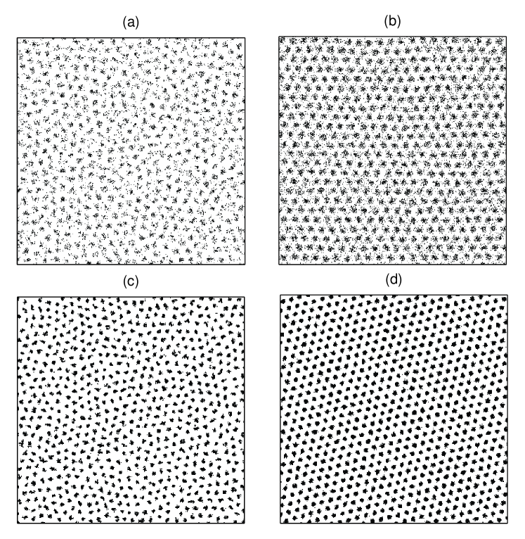
In the active phase, owing to the local-density dependent dynamical rules particles group together forming clusters (see Fig. 1 (a) and (b)) provided that the diffusion constant is small enough (for large values of D, homogeneous distributions are obtained). Such clusters have a well-defined typical diameter (which can be analytically estimated nb ) and a characteristic number of particles within, which depend on the parameters , , and bugs1 ; bugs2 . Well inside the active phase, when the clusters start filling the available space they self-organize in spatial structures with remarkable hexagonal order (see Fig.1 (b)).
From the theoretical side, an important breakthrough is that the IBB model can be cast into a continuous stochastic equation bugs1 . Indeed, by applying standard Fock-space (Doi-Peliti GF ) techniques, a Langevin equation including the main relevant traits of the problem in a parsimonious way can be derived (see Appendix A in bugs1 and references therein). The Langevin equation for the local density density of bugs reads (in the Ito representation)
where the noise amplitude is a function of the microscopic parameters and is a normalized Gaussian white noise. This includes only the leading terms in a density expansion; for instance, a higher order noise term appear in the mapping bugs1 but it does not alter the results reported in what follows in any significant way.
Note that, leaving aside the non-local saturation term, this equation coincides with the Reggeon-field theory or Gribov process, describing at a coarse-grained level systems with absorbing states in the directed percolation (DP) class (see AS and references therein). Let us underline the presence of a square-root multiplicative noise. Note also that the deterministic part of Eq.(II), including a non-local saturation term, is identical to the equation proposed by Fuentes et al. Fuentes . Eq.(II) is therefore a simple (the simplest) stochastic generalization of such model.
The main advantage of the continuous Langevin equation above is that it allows for analytical studies and permits to scrutinize the effect of fluctuations (by just tuning the noise amplitude). It also constitutes a more general, elegant, and compact formulation of the problem. For these reasons, we choose Eq.(II) as the starting point of our forthcoming analyses.
III Integration of the Langevin equation and first analyses
Analytical studies of the deterministic part of Eq.(II) (i.e. mean field analyses) have already been performed in bugs1 ; bugs2 ; Fuentes . They permit, for instance, to understand the wave-length instability mechanism leading to pattern formation, as well as many other aspects. In order to analyze the full stochastic Eq.(II) and, in particular, its associated melting/freezing transition, one needs to resort to computational studies.
However, integrating numerically Langevin equations with square-root noise is a highly non-trivial task; owing to the fact that for small density values the square-root term (with multiplies a random number) becomes larger in amplitude than the deterministic terms, standard integration schemes (Euler, Runge-Kutta, etc.) lead ineluctably to unphysical negative values of the density field dickman , and this pathology is not easily cured in any naïve way. Luckily, a very efficient scheme, specifically devised to overcome such a difficulty, has been recently proposed Dornic .
The method is a split-step algorithm in which the system is discretized in space and two evolution operations are performed at each discrete time-step: (i) first, the noise term is treated in an exact way, by sampling the conditional probability distribution coming out of the (exactly solvable) associated Fokker-Planck equation at each site. By sampling in an exact way such a distribution an output is produced at each site. (ii) Afterwards, the remaining deterministic terms are integrated using any standard scheme taking as the input at each site the output of the previous step at each site. More details and applications can be found in Dornic .
To implement the split-step scheme to integrate Eq.(II) in two dimensions, we discretize the space, by introducing a lattice of linear size or ( is already at the limit of our present computational power). We fix the discrete time step to , , , (which is small enough to have clustering) and use either or as a control parameter. For all of the simulations reported here we initialize the system with a homogeneous initial density, , leave it relax towards its stationary state (reached typically after Monte Carlo steps), and perform steady-state measurements (averaging over, at least, configurations).
First of all, we verify that Eq.(II) reproduces qualitatively all the basic phenomenology of the microscopic IBB model: (i) an absorbing phase for small values of , (ii) an active disordered phase, encountered by increasing for a fixed and (iii) an active ordered crystal-like phase which is reached by further increasing the value of or alternatively, fixing and reducing the noise amplitude, (see Fig.(1 (c) and (d))).
Separating (i) and (ii) there is a directed-percolation-like phase transition, while our focus here is on the transition from the disordered active phase (ii) to the ordered self-organized one (iii). In order to study the effect of the noise on such a transition, from now on, we fix , well into the active phase, and use the noise amplitude, , as a tuning parameter. Fig. 1 (plots (c) and (d)) shows two snapshots obtained for with and respectively. While in both cases clusters of localized activity () exist, only in the second one clusters are self-organized into an ordered hexagonal array.
III.1 Cluster analyses
A preliminary step towards a systematic cluster analysis is to have an efficient method to detect and label them. We have implemented an algorithm, based in the Hoshen-Kopelman one HK as follows. First, to avoid spurious clusters we apply a smoothening filter to the noisy field in our simulations, which removes its short wavelength fluctuations:
| (3) |
where is the cluster average radius (almost constant for the considered parameter range). Then we define a “smoothened” binary field, taking a value () wherever (). The threshold is fixed to an optimal value , found by trial and error, and we verify that an excellent cluster identification (as compared to visual inspection) is obtained. The output is not very sensible to the threshold choice although small variations can be observed. Once the binary discretized field has been constructed, a standard Hoshen-Kopelman algorithm is straightforwardly employed. It generates a list of clusters, together with the list of spatial coordinates ascribed to (the center of mass of) each of them.
Having described the main computational techniques, we now report on various observables characterizing collective properties of clusters.
The average cluster mobility, , is defined as the standard deviation of the excursion of the cluster center of mass (during a fixed-length time interval), averaged over many different clusters in the steady state
| (4) |
where are the center of mass cluster coordinates and stands for averages in the steady state.
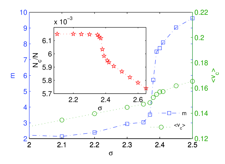
In Fig. 2 we plot as a function of the noise amplitude ; the mobility exhibits a sharp transition (sharper upon enlarging the system size) from the low-noise phase in which the clusters are almost frozen and localized in space to the high noise one in which they move more freely. The change of behavior occurs around .
Fig. 2 shows also the average velocity (in modulus) of the cluster center of mass versus . While for small values of we observe a linear dependence between and linear , this linear dependence is broken above certain noise threshold (again around ), at which its derivative exhibits a discontinuity. Above the transition point the velocity increases non-linearly with .
We have also measured (Fig.2 inset) the number of clusters per surface unit as a function of . While in the disordered phase the density of clusters increases as the noise strength is reduced, it remains constant (at a value corresponding to the maximum capacity) once the threshold for an ordered structure is reached.
The three described observables provide evidence of a melting/freezing transition. The change of behavior occurs in all cases at a unique point, somewhere around . A more detailed finite size scaling analysis would be required to pin down the critical point with more accuracy using these observables.
The picture that emerges from these measurements is that clusters emerge at a mesoscopic scale out of the nonequilibrium microscopic rules and then, upon reducing the noise-amplitude, they self-organize into frozen patterns with reduced mobility and velocity and with a more compact packing. In this sense, clusters become the equivalent of “particles” in standard liquid/solid transitions.
III.2 Structure Function Analysis.
In order to obtain an alternative, more direct, estimation of the location of the freezing/melting transition not relying on the (computationally costly) identification of clusters, we analyze a properly defined structure function. As the overall density varies upon changing parameters and system size, it is convenient to define a normalized version of the structure function as follows
| (5) |
where is the Fourier transform of the normalized density
| (6) |
is the momentum, stands for spherical averages over all two-dimensional vectors with module , and the normalized density is
| (7) |
Using this normalized density, and by virtue of the Parseval’s identity, it is guaranteed that is normalized to unity for all parameter values and system-sizes.
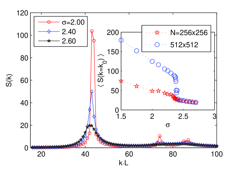
Fig.3 shows the structure-function for a size as a function of , for three different noise amplitudes: and . The three curves exhibits a very pronounced first Bragg-peak at positions around (which corresponds to and therefore a separation between clusters . Their respective heights decrease with noise strength: the larger the noise the less ordered the structure. Nevertheless, perfect ordering (delta-peak at a given mode) will never be reached as cluster internal fluctuations enforce some dispersion in the structure function.
Given that has been normalized, the height at , , constitutes a good measure of the degree of order. Actually, an abrupt transition is obtained at about for the largest available size (see (Fig.3)): above the transition decreases abruptly corresponding to the breakdown (melting) of the ordered patterns. Also, observe in the inset of Fig.3 that the degree of order is enhanced upon enlarging the system size from to . We will come back to analyze this issue later.
IV Two-dimensional melting theories: a short review
The evidence accumulated so far, both from cluster analyses and structure function measurements, reveals the existence of a melting/freezing transition, somewhere around . The key question we face now is: does such a nonequilibrium transition exhibit the well-known universal features of standard equilibrium melting/freezing in two-dimensional systems?
Note, in addition, that here the number of clusters (particles) is not constant but fluctuates, and its average value varies as a function of the control parameter, . Is this relevant for the properties at the melting/freezing transition?
Before tackling these problems, for the sake of completeness, and for future reference, in this section we briefly summarize the main results of the celebrated standard theory of two-dimensional melting: the Kosterlitz-Thouless-Halperin-Nelson-Young (KTHNY) theory KT ; KTHNY ; Strandburg ; Nelson . We also discuss briefly an alternative competing theory.
The KTHNY is based on a statistical physics analysis of topological defects, i.e. particles with a number of nearest neighbors (assuming a Voronoi or Wigner-Seitz construction) other than . Dislocations perturb translational order and disclinations hinder orientational order Nelson ; Strandburg . A detailed inspection of hexagonal ordering in the presence of fluctuations reveals that disclinations correspond to free monopoles, either five-fold or seven-fold, where five and seven refer to the number of nearest neighbors as measured in a Voronoi or Wigner-Seitz construction. Analogously, dislocations can be identified with tight pairs (i.e. dipoles) of a five-fold and a seven-fold disclinations. The disordered (or isotropic or liquid) phase is characterized by the proliferation of defects: both monopoles and dipoles.
The main prediction of the KTHNY theory is that, contrarily to what happens in higher dimensional systems, where the melting occurs discontinuously at a unique transition point, in two-dimensional systems melting occurs in two stages. Translational and orientational order lose their stability at different Kosterlitz-Thouless-like KT critical points where dislocations and disclinations, respectively, unbind.
The theory assumes that in the solid phase there are nor free dipoles nor monopoles, but only quadrupoles (low-energy excitations), that the number of dislocations/dipoles throughout the first (melting) transition is small and that they are generated progressively in a smooth way as the temperature is risen. This allows to treat the system at the melting transition as a weakly interacting gas of dipoles/dislocations. An analogous assumption is made for monopoles/disclinations at the second transition point where monopoles unbind from dipoles.
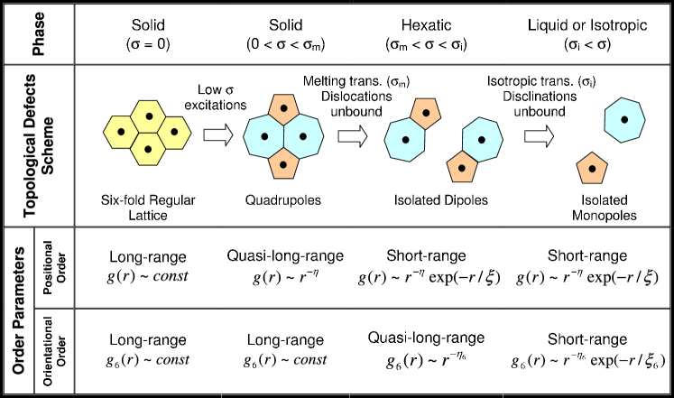
The three phases put forward by the KTHNY theory are as follows KTHNY ; Strandburg ; Nelson (see Fig. 4 for a graphical illustration):
-
•
Only at zero temperature the lattice ordering can be perfect while, for any non-vanishing temperature, defects appear. Below a first critical point (denoted here) defects are tight together in quadrupoles, hindering translational order. As a result, translational correlation functions decay algebraically in space (with continuously varying exponents), as corresponds to quasi long-range order. Orientational correlations (see below for a precise definition) decay at long distances to a non-vanishing constant value, corresponding to true long-range orientational order explanation .
-
•
Above a first critical point, , dipoles/dislocations unbound from quadrupoles, destroy translational order (i.e. translational correlations decay exponentially fast). They also affect orientational correlations which decay algebraically with a continuously variant exponent obeying and a diverging correlation length, i.e. they exhibit quasi-long-range orientational order. This is the, so called, hexatic phase.
-
•
Above a second (isotropic) critical point, , monopoles/disclinations unbind from dipoles, hindering quasi long range orientational order. Both translational and orientational correlations decay exponentially. The associated correlation lengths diverge as stretched exponentials of the form where is the distance to . This is the isotropic (also called disordered or liquid) phase.
This scenario has been verified in a number of numerical Hexatic ; Strandburg and experimental Hexatic-exp ; Strandburg studies, while it was not verified in others JJ ; QG .
Despite of its success, the KTHNY is not the only plausible theory of two-dimensional melting. A competing one was proposed by Chui Chui , who argued that some systems should exhibit a unique first-order melting transition mediated by the appearance of “grain boundaries”. In this picture, chains of defects appear limiting ordered grains and separate neighboring mismatching domains. The main difference between this theory and the KTHNY one is that here the transition appears owing to a collective excitation of defects. In some systems, it has been shown that the melting transition can change from KTHNY to first order upon changing some parameter Strandburg , so both theories can be taken as complementary.
V Analysis of the nonequilibrium melting/freezing transition
To determine the plausibility of the KTHNY scenario (or, instead, that of competing theories) for the nonequilibrium transition under study, we analyze in this section translational and orientational order in numerical simulations of Eq.(II).
V.1 Translational Order
Translational order can be studied by measuring the two-point radial correlation function:
| (8) |
where stands for averages in the stationary state taken over all pairs of particles at generic positions r and separated by a distance .
In Fig.5 we plot as a function of for different values of above and below the critical point. For all parameter values the wavy curves reveal the clustered nature of the density distribution. To determine their asymptotic trends, we analyze the envelope of such curves, and fit it to the behavior predicted by the KTHNY theory:
| (9) |
where and are fitting parameters. Note that, the power-law corresponds to the KTHNY prediction while the exponential allows to describe finite-size induced cut-offs. Fig.6 shows the results of such a fit for different values of . In all cases, the fit correlation coefficient is large than . Note first the abrupt jump of the translational correlation length at the critical value ; in the ordered phases it converges to a saturation value controlled by system size (see figure caption), while in the disordered one it takes much smaller values. On the other hand, the exponent changes continuously from a value nearby at the critical point (in perfect agreement with the KTHNY prediction, which imposes ) to smaller values as is decreased, confirming the generic algebraic decay of in the solid phase, with an exponential cut-off given by the system size.
To check the internal consistency of our results, we also estimate by analyzing the previously obtained structure-function results. As is trivially related to through a Fourier transform, and (which depends only on the modulus of , ) can be modeled in the solid phase by (for simplicity, we omit here the exponential, system size induced, cut-off ) one can find after simple algebra, that for a two-dimensional system of size
| (10) |
where is the zero-order Bessel function. Using the asymptotic behavior of it is not difficult to obtain that
| (11) |
for the mode (which is the only one for which there are not destructive interferences).
Actually, in the inset of Fig.(3) we showed that while the curves for overlap for different system sizes above the critical point, bellow it, they growth with system size. Indeed they grow algebraically with a slightly -dependent exponent which for all values is in the interval . Therefore, exploiting Eq.(11) we derive a value for which is in the interval in rather good agreement with the direct measurements above. Summing up, we have deduced, in two independent ways, results consistent with algebraically decaying correlations as predicted by the KTHNY scenario.
V.2 Orientational Order
To quantify the degree of orientational order of a given configuration in the steady state, we first identify the clusters using the algorithm described above. After that, a Voronoi tessellation of the system configuration is constructed Voronoi . For each configuration, the corresponding tessellation gives as output the list of clusters and the set of nearest neighbors of each. Finally, for each cluster , we define Strandburg ; KTHNY ; Nelson
| (12) |
where the sum extends over the neighbors of cluster ; is the angle between the centers of mass of clusters and and an arbitrary fixed reference axis. The average of over different clusters,
| (13) |
where is the total number of clusters, is a global orientational order parameter. An associated susceptibility can be also defined,
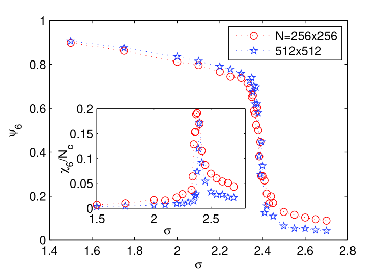
Fig. 7 (main plot) shows as a function of for two different system sizes. For , changes abruptly in the interval from a large value for below to relatively small ones above . Note that finite size effects operate in opposite directions below and above the transition and the curves intersect at some point between these two regimes (resembling what happens for the Binder cumulant at continuous phase transitions). This provides a useful criterion to locate the critical point; using the two available sizes, the best estimation is , and strongly suggests that the transition is continuous in agreement with the KTHNY scenario. On the other hand, the susceptibility (inset of Fig. 7) exhibits a sharp peak, which moves slightly to the right with increasing system size, being located at for .
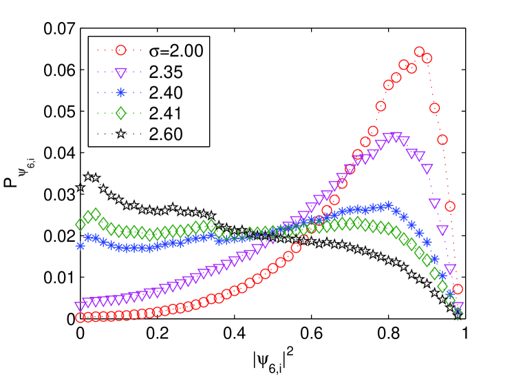
The probability distribution function (pdf) of provides additional information about the nature of the transition. In Fig. 8 we plot the pdf as a function of (to have only positive values) for various and size . At small values of (as or ) the pdf is unimodal and peaked around a high value. Increasing the noise strength the peak becomes less pronounced. For noise values around the transition point, the pdfs are rather flat, a new peak appears nearby zero, and the average value shift (in an apparently continuous way) from a high value in the ordered phase to a small one in the disordered one.
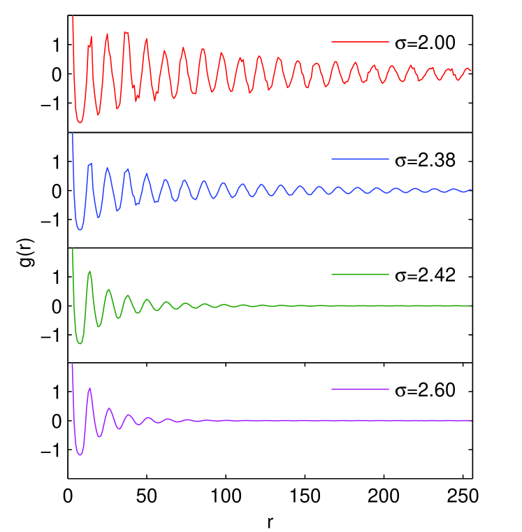
To further check the predictions of the KTHNY theory it is necessary to determine the two-point orientational correlation function:
| (14) |
where the average is taken over all pairs of clusters separated by a distance (results shown in Fig. 9).
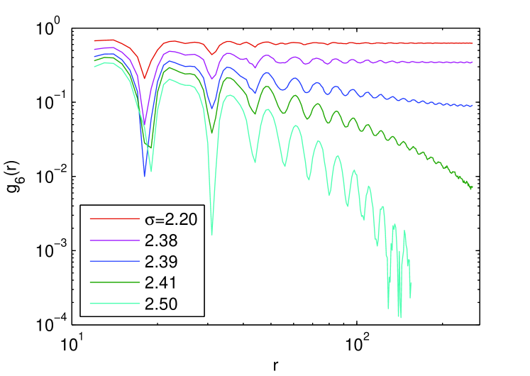
While for the envelope of the curves veers down in a double-logarithmic plot (i.e. decay exponentially) for values smaller than the envelopes converge to constant values in the long distance limit, signaling the emergence of true long-range orientational order in the crystal-like phase. We find no evidence of a hexatic phase, characterized by generic power-law decaying orientational correlations. If it actually exists it should be very narrow and could not be detected within our present numerical resolution. Indeed, we have scanned in steps of units (not shown), and we always find that the envelopes either bend down below certain separatrix (i.e. the critical point, which here we estimate to be at ) or flatten above such a value.
V.3 Analysis of the isotropic phase
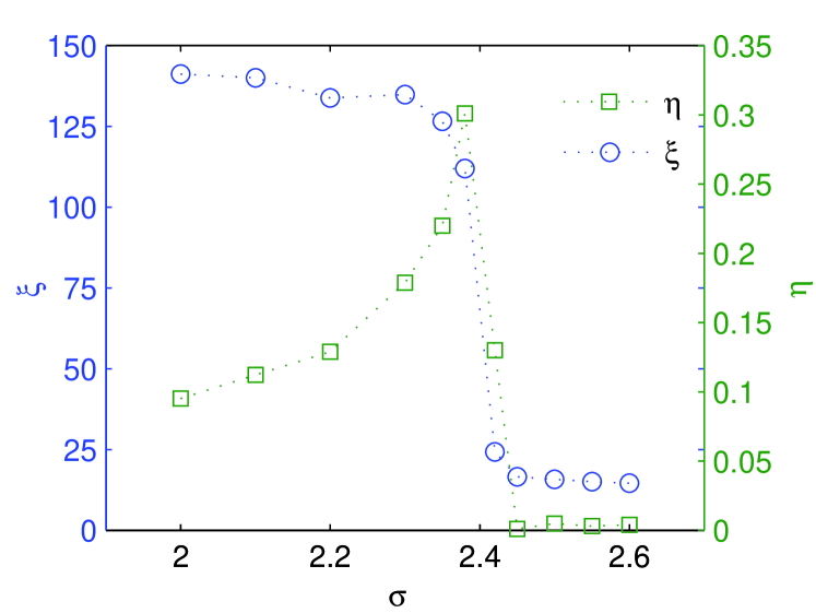
As synthesized above, the KTHNY theory predicts that in the disordered or isotropic phase KTHNY ; Strandburg ; Nelson
| (15) |
where is a critical exponent and , the orientational correlation length. The theory also predicts a divergence in as the critical point is approached
| (16) |
where is the distance to the critical point and and are constants. A similar, stretched exponential behavior is also predicted for the susceptibility, .
Both and can be measured by fitting the envelopes of for different values of to Eq.(15). We have performed a two-parameter ( and ) fit, and obtain the results summarized in Table 1. Observe the very fast grow of upon approaching the transition point. The estimations of are very close to the KTHNY value (actually, they become indistinguishable by including error-bars). Not surprisingly, close to the critical point, the correlation coefficient, , is worse than far from it.
| 2.39 | 291.8 | 0.320 | 0.977 |
| 2.41 | 70.5 | 0.298 | 0.997 |
| 2.45 | 47.8 | 0.299 | 0.995 |
| 2.50 | 30.6 | 0.261 | 0.998 |
| 2.55 | 24.1 | 0.245 | 0.997 |
| 2.60 | 22.5 | 0.254 | 0.996 |
In Fig. 10 we show the results obtained by fitting the simulation results to the predicted stretched exponential behavior Eq.(16). The fit is excellent in both cases and allows for estimations of the critical point location: using and using .
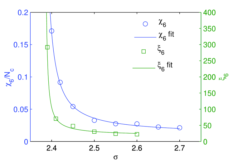
These results provide a strong backing for a KTHNY scenario in the isotropic phase.
V.4 Summary of the numerical observations
Summing up, the numerical analyses detailed above are consistent with the KTHNY theory in any respect, except for the fact that no evidence of a hexatic phase is found. Our results are compatible with a scenario very similar to the KTHNY one, but with the two transition points merging into a unique one, occurring somewhere between and . No evidence is found of a hexatic phase. A scenario analogous to this, i.e. a one-stage continuous melting transition, has been found in other equilibrium and nonequilibrium systems JJ ; QG .
VI Defect analysis
Inspired by the analyses in QG , in this section we check the KTHNY assumptions rather than its predictions. As briefly explained above, the theory assumes that the number of dipoles/dislocations (monopoles/disclinations) throughout the first (second) transition is small and that they are generated progressively in a smooth way as the temperature is risen. This allows to treat the first (second) transition as a weakly interacting gas of dipoles/dislocations (monopoles/disclinations).
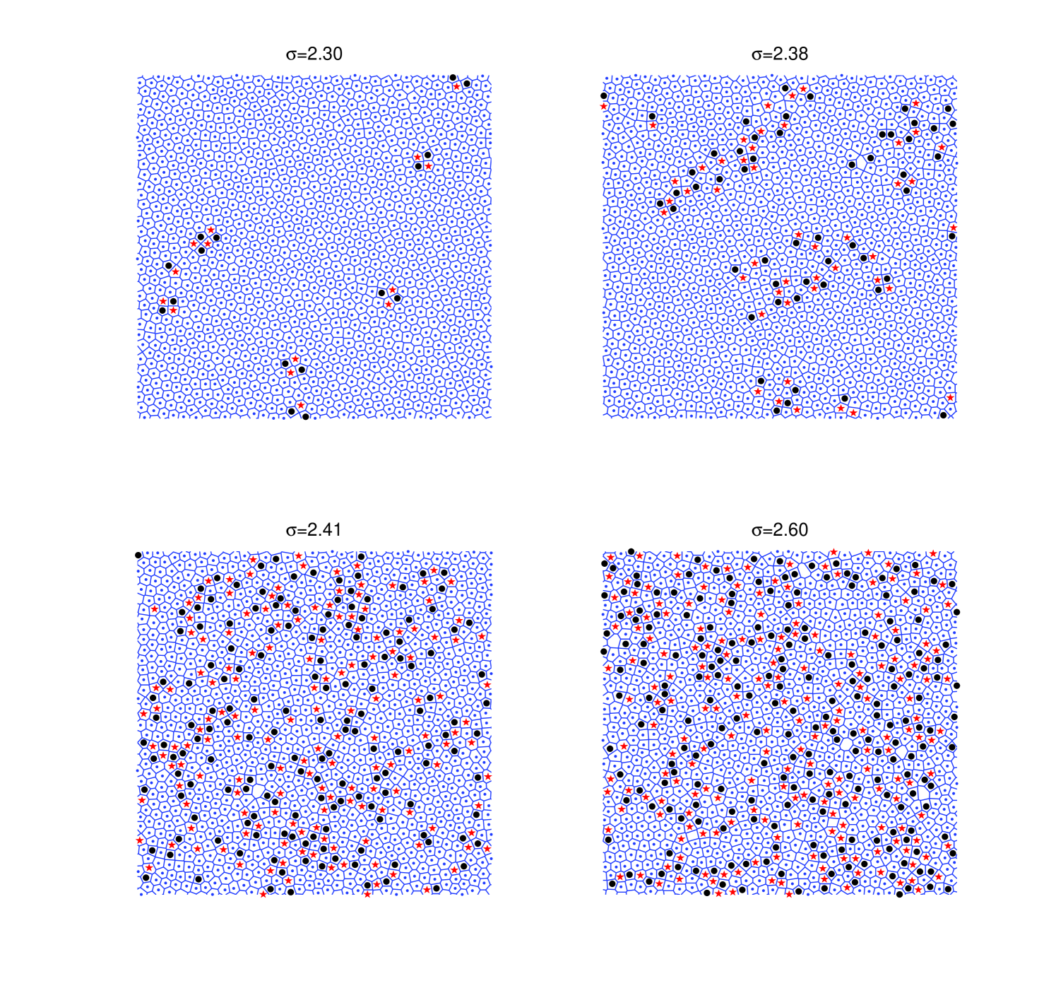
To check if this picture describes properly the behavior of our model, we scrutinize how defects appear and proliferate upon rising the noise amplitude. In Fig. 11 we plot defect maps for different values of . The lines correspond to the Voronoi construction for a given configuration; five-fold, six-fold, and seven-fold clusters are marked with black circles, central dots, and red stars respectively (higher and lower order defects correspond to blank clusters). As the noise amplitude is increased the total number of defects grows. While below the critical point only quadrupoles are significatively present, nearby the transition point isolated dipoles start unbinding. Even if unbound, they have a clear tendency to bunch together, and indeed, at slightly larger noise-amplitudes, in the isotropic phase, defects bunch together showing a tendency to form string-like structures. Deep into the isotropic phase defects proliferate, and extend through the system keeping, in any case, the propensity to form condensed string-like structures.
In this respect, it is noteworthy that Fisher, et al. Fisher predicted, within the KTHNY theory, that monopoles can appear at correlated locations showing a strong tendency to arrange themselves in small-angle grain boundaries. Contrarily, the condensates we find seem to be dominated by strings of dipoles.
To quantify the phenomenology above, we measure the density of defects (quadrupoles, dipoles and monopoles) as a function of noise amplitude (see Fig.12). The density of defects (of any type) grows from a small value below to a large value in the isotropic phase. The increase is very steep around for both dipole and monopole densities, suggesting the existence of a unique unbinding transition.
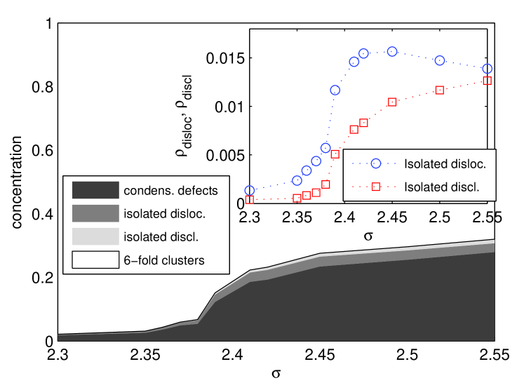
To complement the previous plot, the inset of Fig. 12 shows the density of isolated dipoles/dislocations and monopoles/disclinations versus , confirming the previous observations, that the steepest increase occurs at . Note that the total number of monopoles grows continuously upon increasing , while the presence of a relative maximum in the density of dipoles reflects the competition between two conflicting tendencies: the unbinding of dipoles from quadrupoles and the liberation of monopoles (and formation of condensed defects) from free dipoles.
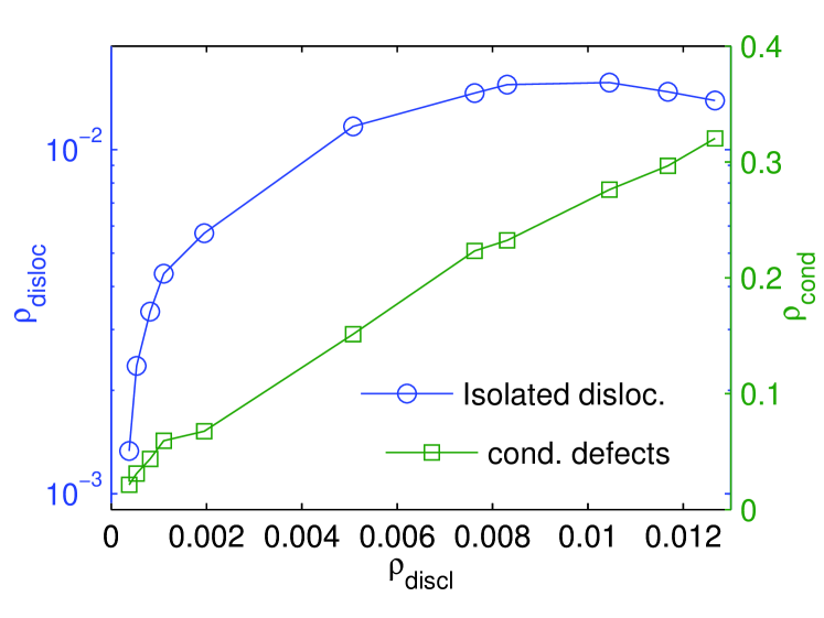
Finally, Fig. 13 shows the densities of isolated dipoles and of condensates as a function of the density of monopoles. This plot reveals a strong correlation between monopoles and dipoles and, more importantly, it illustrates how they both vanish at roughly the same point, suggesting again (up to finite size effects) the existence of a unique one-stage transition. Indeed, if the dipoles unbinding occurred before the monopoles one, the line joining the circles should intersect the vertical axis which is not the case. It is also at such a unique transition point that condensed defects appear, being their density (roughly) linearly correlated with the density of monopoles.
In summary, a detailed analysis of defects in Voronoi tessellations supports the interpretation that both dipoles and monopoles unbind at a unique critical point. At such a transition point condensed defects are generated in an apparently continuous way. In a future publication we will analyze in a more detail the correlations between isolated monopoles, dipoles and condensates to further clarify the analogies and differences with the standard KTHNY scenario, and try to develop a theoretical framework for one-stage continuous melting transitions.
VII Discussion and Conclusions
Motivated by the observation of remarkably regular arrays of clusters formed by bacteria growing in Petri dishes and related problems, we have revisited the individual-based interacting Brownian bug (IBB) model in which birth rates are local-density dependent bugs1 ; bugs2 . Apart from an absorbing phase transition, this model shows a transition from a disordered active phase, in which particles aggregate in localized clusters, to an ordered or crystallized active phase, in which clusters self-organize forming hexagonal arrays. For the sake of generality and aimed at facilitating analytical studies, rather than studying the discrete model itself we have analyzed its equivalent continuous Langevin representation. This stochastic equation, which involves a non-local saturation term as well as a square-root multiplicative noise, can be numerically integrated by discretizing it and employing a recently introduced efficient integration scheme specifically designed to deal with square-root multiplicative noise Dornic .
The main results we obtain are:
(i) First, we have shown explicitly that the continuous model (truncated to include only the leading terms) reproduces the phenomenology of the original discrete model, including an absorbing phase in which the stationary particle density is zero, a disordered active phase in which the density field is localized in clusters of activity surrounded by empty regions and, finally an ordered phase with hexagonal patterns.
(ii) We have studied the ordering transition by analyzing cluster properties (average velocity, mean-displacement, etc.) as well as by means of analyses of the structure-function. These studies reveal that a melting/freezing transition indeed occurs at some value of the noise amplitude: for small noises, clusters are trapped into hexagonal configurations as a result of a collective effect, while for noise amplitudes above threshold they have much more mobility.
(iii) To better understand and quantify the transition we have studied both translational and orientational correlation functions. In particular, we have verified that, in the solid phase, translational correlation functions exhibit generic power-law decay even if with system-size induced cut-offs. The value of the decay exponent at the melting transition being in excellent agreement with the KTHNY prediction. However, we do not found any evidence of an hexatic phase, contrarily to what predicted by the standard (Kosterlitz-Thouless-Halperin-Nelson-Young (KTHNY)) theory. This same conclusion is also borne out by analysis of the global orientational order-parameter. Up to the numerical resolution limit, this suggests the existence of a unique continuous transition point.
(iv) Above such a transition point, i.e. in the disordered or isotropic phase, the correlation functions have been shown to decay as stretched exponentials, in excellent agreement with the KTHNY predictions.
(v) We have performed a detailed analysis of defects and found that both free dipoles/dislocations and monopoles/disclinations seem to unbind from quadrupoles at a unique transition point, above which also defect condensates are formed. This is in contrast with the KTHNY scenario and leads to a continuous one-stage melting transition.
(vi) The unique transition is continuous, so it cannot be explained by the main alternative theory to KTHNY Chui which predicts a first-order melting transition.
Summing up, the phenomenology of this nonequilibrium model can be only partially described by the KTHNY theory. While the melting/freezing transition is indeed characterized by the smooth unbinding of defects this occurs through a unique continuous transition. The reason for this seems to yield in the fact that once dipoles/dislocations unbind, the perturbation they generate around them is large enough as to unbind also monopoles/disclinations: dipoles, monopoles and the string-like condensates they form are strongly correlated.
Note that, the nonequilibrium microscopic dynamics of the interacting Brownian bug model (or its equivalent Langevin representation) is responsible for the generation of mesoscopic clusters. Once such clusters are generated, they interact in an effective way, and the physics at a macroscopic scale does not seem to differ in any essential way from other equilibrium problems JJ ; QG for which a similar one-stage continuous melting transition has been reported. We believe that this scenario is not specific of nonequilibrium systems but is determined by the way in which defects interact among themselves. This might not depend on the equilibrium versus nonequilibrium nature of the process but rather on other structural details influencing the way defects interact among themselves. A more detailed analysis of defects and defect-correlation will be investigated in a future work, where we will try to develop a theoretical framework for one-stage continuous melting transitions.
Let us also emphasize that the models we have analyzed are not the best choice to explore with high numerical resolution the possibility of one-stage melting from a general perspective. Effective models,with a dynamics at the level of clusters (as opposed to having a microscopic dynamics for particles) would be a much better option from the computational point of view.
In summary, despite of interesting and not fully understood differences, the striking patterns produced by the biologically inspired Langevin equation (II) resemble very much the melting/freezing solid/liquid transition in equilibrium systems.
It is our hope that this paper will motivate further studies of (i) the effect of fluctuations on self-organized nonequilibrium patterns and (ii) the analogies and differences between the defect-mediated type of melting transition described here and standard equilibrium melting scenarios.
ACKNOWLEDGMENTS We acknowledge useful comments and discussions with F. de los Santos. This work was supported in part by the Spanish projects FIS2005-00791 and FIS2004-00953 (Ministerio de Educación y Ciencia), FQM-165 (Junta de Andalucía), and the European Commission through the NEST-Complexity project PATRES (043268).
References
- (1) J. D. Murray, Mathematical Biology, Berlin, Springer-Verlag, 1989.
- (2) G. Flierl, D. Grünbaum, S. Levin, and D. Olson, J. Theor. Biol. 196, 397 (1999).
- (3) A. P. Martin, Progr. in Oceanography, 57, 125 (2003).
- (4) Spatial Ecology, Ed. by D. Tilman and P. Kareiva, (Princeton University Press, Princeton, 1997). J. von Hardenberg et al, Phys. Rev. Lett. 87, 198101 (2001).
- (5) E. O. Budrene and H. C. Berg, Nature, 349, 630 (1991); ibid. 376, 49 (1995). D. E. Woodward et al., Biophys. J. 68, 2181 (1995).
- (6) E. Ben-Jacob, I. Cohen, H. Levine. Adv. Phys. 49, 395 (2000).
- (7) J. M. Deutsch, J. Phys. A 18, 1449 (1985). M. Wilkinson and B. Mehlig, Phys. Rev. E 68, 040101(R) (2003). T. Tél, A. de Moura, C. Grebogi, and G. Károlyi, Phys. Rep. 413, 91 (2005).
- (8) W. R. Young, A. J. Roberts, and G. Stuhne, Nature, 412, 328 (2001). See also, Y-C. Zhang, M. Serva, and M. Polikarpov, J. Stat. Phys. 58, 849 (1990). M. Meyer, S. Havlin, and A. Bunde, Phys. Rev. E 54, 5567 (1996). B. Houchmandzadeh, Phys. Rev. E 66, 052902 (2002). J. Felsenstein, Amer. Natur. 109, 359 (1975).
- (9) M. C. Cross and P. C. Hohenberg, Rev. Mod. Phys. 65, 851 (1994).
- (10) D. Walgraef, Spatio-Temporal Pattern Formation, Springer-verlag, New York, 1997.
- (11) M. A. Fuentes, M. N. Kuperman, and V. M. Kenkre, Phys. Rev. Lett. 91, 158104 (2003). Related works are: H. Sayama, M. A. M. de Aguiar, Y. Bar-Yam, and M. Baranger, Phys. Rev. E 65, 051919 (2002); Y. E. Maruvka and N. M. Shnerb, Phys. Rev. E 73, 011903 (2006).
- (12) D. H. Janzen, American Naturalist, 104, 501 (1970). For an updated review see, Tropical Forest Diversity and Dynamism, Ed. E. C. Losos and E. G. Leigh, Jr. Chicago University Press, Chicago, 2004.
- (13) T. Vicsek, A. Czirok, E. Ben-Jacob, I. Cohen, and O. Shochet, Phys. Rev. Lett. 75, 1226 (1995). See also, G. Gregoire and H. Chaté, Phys. Rev. Lett. 92, 25702 (2004). G. Gregoire, H. Chaté, and Y. Tu, Physica D 181, 157 (2003). E. V. Albano, Phys. Rev. Lett. 77 2129 (1996).
- (14) N. D. Mermin and H. Wagner, Phys. Rev. Lett. 17, 1133 (1966). P. C. Hohenberg, Phys. Rev. 158, 383 (1967). N. D. Mermin, Rev. Mod. Phys. 51, 591 (1979).
- (15) J. M. Kosterlitz and D. J. Thouless, J. Phys. C 6, 1181 (1973).
- (16) B. I. Halperin and D. R. Nelson, Phys. Rev. Lett. 41, 121 (1978). D. R: Nelson and B. I. Halperin, Phys. Rev. B 19, 2457 (1979). D. R: Nelson and B. I. Halperin, 21, 5312 (1980). A. P. Young, Phys. Rev. B 19, 1855 (1979).
- (17) K. J. Strandburg, Rev. Mod. Phys., 60, 161 (1988).
- (18) D. R. Nelson, Defects and Geometry in Condensed Matter Physics, Cambridge University Press, Boston (2002).
- (19) S. T. Chui, Phys. Rev. Lett. 48, 933 (1982); Phys. Rev. B 28, 178 (1983). See also, M. A. Glaser and N. A. Clark, Adv. Chem. Phys. 83, 543 (1993).
- (20) H. Hinrichsen, Adv. Phys. 49, 815 (2000). G. Grinstein and M. A. Muñoz, in Fourth Granada Lectures in Computational Physics, Ed. P. L. Garrido and J. Marro, Springer, Berlin, 1997. G. Odor, Rev. Mod. Phys. 76, 663 (2004).
- (21) J. Toner and Y. Tu, Phys. Rev. Lett. 75 , 4326 (1996). J. Toner, Y. Tu, and S. Ramaswany, Ann. of Phys. 318, 170 (2005).
- (22) K. E. Bassler and Z. Rácz, Phys. Rev. E 52, R9 (1995).
- (23) E. Hernández-García and C. López, Phys. Rev. E 70, 016216 (2004).
- (24) C. López and E. Hernández-García, Physica D 199, 223 (2004). E. Hernández-García and C. López, J. Phys. Cond. Matt. 17, S4263 (2005).
- (25) C. López, F. Ramos, and E. Hernandez-García, J. Phys.(Condensed Matter) 19, 065133 (2007 ).
- (26) J. F. Fernández, J. J. Alonso, and J. Stankiewicz, Phys. Rev. Lett. 75, 3477 (1995). Phys. Rev. E 55, 750 (1997). J. J. Ruiz-Lorenzo, E. Moro, and R. Cuerno, Phys. Rev. E 73, 015103(R) (2006).
- (27) R. A. Quinn and J. Goree, Phys. Rev. E 64 051404 (2001).
- (28) B. M. Bolker and S. W. Pacala, Theor. Pop. Biol. 52 179 (1997). D. Birch and W. R. Young, J. Theor. Pop. Biol. 70, 26 (2006). C. López, Phys. Rev. E 74, 012102 (2006).
- (29) Since the only factor impeding unbounded diffusive spreading of particles is their finite lifetime which, in its turn, is proportional to the inverse of the death rate, , the average linear size of clusters has to be proportional to , as can be numerically verified bugs1 ; bugs2 .
- (30) M. Doi, J. Phys. A 9, 1479 (1976). L. Peliti, J. Physique, 46, 1469 (1985). P. Grassberger and M. Scheunert, Fortschr. Phys. 28, 547 (1980). C. J. DeDominicis, J. Physique 37, 247 (1976). H. K. Janssen, Z. Phys. B 23, 377 (1976).
- (31) Strictly speaking, when employing the Doi-Peliti formalism the resulting field is not a density field, but its first moment coincide with the density GF .
- (32) R. Dickman, Phys. Rev. E 50, 4404 (1994). C. López and M. A. Muñoz, Phys. Rev. E 56, 4864 (1997).
- (33) I. Dornic, H. Chaté, and M. A. Muñoz, Phys. Rev. Lett. 94, 100601 (2005). See also, L. Pechenik and H. Levine, Phys. Rev. E 59, 3893 (1999). E, Moro, Phys. Rev. E 70, 045102(R) (2004).
- (34) J. Hoshen and R. Kopelman, Phys. Rev. B 14 3438 (1976).
- (35) The linear dependence in the ordered phase can be interpreted as a direct transfer of the “thermal” energy introduced by the noise to the kinetic energy of clusters.
- (36) Orientational ordering escapes the premises of the MWH theorem. Indeed, the local hexagonal ordering induces an effective long-range interaction not covered by the theorem hypotheses.
- (37) A. Jaster, Phys. Rev. E 59, 2594 (1999); Phys. Lett. A 330, 120 (2004). K. Chen, T. Kaplan, and M. Mostoller, Phys. Rev. Lett. 74, 4019 (1995). K. Bagchi, H. C. Andersen, and W. Swope, Phys. Rev. Lett. 76, 255 (1996). R. Radhakrishnan, K. E. Gubbins, and M. Sliwinska-Bartkowiak, Phys. Rev. Lett. 89, 076101 (2002). C. H. Mak, Phys. Rev. E 73, 065104(R) (2006). S. Z. Lin, B. Zheng, and S. Trimper, Phys. Rev. E 73, 066106 (2006).
- (38) J. D. Brock, R. J. Birgenau, J. D. Lister, and A. Aharony, Phys. Today 42, 52 (1989). C. F. Chou, A. J. Jin, S. W. Hwang, and J. T. Ho, Science 280, 1424 (1998).
- (39) A. Okabe, B. Boots, and K. Sugihara, Spatial Tessellations, Concepts and Applications of Voronoi diagrams, John Wiley and Sons Ltd. England (1992). J. R. Sack and J. Urrutia, Handbook of Computational Geometry, Elsevier Science, Netherlands (2000).
- (40) D. S. Fisher, B. I. Halperin, and R. Morf, Phys. Rev. B 20, 4692 (1979).