CSS_J154915.7+375506: A low-mass-ratio marginal contact binary system with a hierarchical third body

Jin-Feng Wu,¹²³ Li-Ying Zhu,¹²³ Azizbek MATEKOV,¹²⁴ Lin-jia Li,¹³ Shuhrat EHGAMBERDIEV,⁴⁵ Ildar ASFANDIYAROV,⁴ Jiang-Jiao Wang,¹²³ Jia Zhang¹³ and Fang-Bin Meng¹²³
¹Yunnan Observatories, Chinese Academy of Sciences (CAS), Kunming 650216, China
²University of Chinese Academy of Sciences, No.1 Yanqihu East Rd, Huairou District, 101408, Beijing, People’s Republic of China
³Key Laboratory of the Structure and Evolution of Celestial Objects, Chinese Academy of Sciences, 650216, Kunming, People’s Republic of China
⁴Ulugh Beg Astronomical Institute of the Uzbekistan Academy of Science, Astronomicheskaya 33, Tashkent, 100052, Uzbekistan
⁵National University of Uzbekistan, 4 University str, Tashkent, 100174, Uzbekistan
E-mail: wujinfeng@ynao.ac.cnE-mail: zhuly@ynao.ac.cn

(Last updated 2020 June 10; in original form 2013 September 5)

Abstract

We presented the multi-filter light curves of CSS_J154915.7+375506 inaugurally, which were observed by the 1.5 m AZT-22 telescope at Maidanak Astronomical Observatory. A low-resolution spectrum obtained by LAMOST reveals it is an A-type close binary. By analyzing the BVRI total-eclipse light curves, we are able to derive a reliable photometric solution for this system, which indicates that CSS_J154915.7+375506 is an extremely low-mass-ratio (q=0.138) marginal contact binary system. The location in the HR diagram shows that its secondary component with a much smaller mass is the more evolved one, indicating the mass ratio reversal occurred. The present secondary component had transferred a significant amount of mass to the present primary one. By the combination of a total of 20 times of minimum, we investigated its O-C curve. A periodic oscillation and a possible period decrease have been detected. As the period decreases, the system will evolve towards the contact phase. This makes CSS_J154915.7+375506 a valuable case to study the formation scenario of contact binaries through mass reversal. The periodic oscillation suggested a third body with a minimal mass of $0.91\,M_{\odot}$ , which is larger than that of the less massive component in the central binary. This implies that the secondary body was not replaced by the third body during early stellar interactions, indicating that it is a fossil system and retains its original dynamical information.

keywords:

binaries:close – binaries:eclipsing – stars:evolution – stars:individual(CSS_J154915.7+375506)

^†^†pubyear: 2020^†^†pagerange: CSS_J154915.7+375506: A low-mass-ratio marginal contact binary system with a hierarchical third body–References

1 Introduction

Eclipsing binary systems exhibiting EB-type light variations, particularly those of short periods, offer captivating insights into the evolutionary transformations experienced by close binary systems. Near-contact binaries(NCBs), an important subclass of close binaries which lie in a key evolutionary stage(Zhu & Qian, 2006), were defined by(Shaw et al., 1994). Considering the geometric structure of NCBs, it can be divided into 4 subclasses: SD1 type or SD2 type, semi-detached binaries with star1 or star2 filling its critical Roche lobe; D type, detached binary with components very close to their critical Roche lobe; and C type, marginal contact binary, both components filling their critical Roche lobe with large temperature differences(Zhu & Qian, 2009). The marginal contact system is considered a special type of NCB in testing the Thermal relaxation oscillation (TRO) theory (Lucy, 1976a; Lucy & Wilson, 1979; Flannery, 1976). On the basis of TRO theory, the long-term instability of thermal equilibrium in contact configurations results in the status of marginal contact, together the semi-detached constitute two phases of periodic thermal relaxation oscillation. NCBs which lie in these two phases that sustain such a short time compared to the lifetime of the binary, are rare. So, despite decades of comprehensive research, the properties and evolution on marginal contact binaries still remain blurred. A recently formed contact binary will undergo thermal evolution towards a state of marginal contact, and if the contact is subsequently disrupted, the system will revert back into contact(Lucy, 1976b). This implies that a marginal contact binary could represent a pre-contact binary system. The transitional nature of marginal contact binaries is a crucial evolutionary stage that has the potential to enhance our understanding of the evolutionary process of NCBs. Building on this, K. Stepien and M. Kiraga’s evolutionary model(Stępień & Kiraga, 2013)suggests that contact binaries may have experienced mass ratio reversal in the past. Based on the discussion of marginal contact binaries above, we will now introduce our upcoming research, which will delve into a specific marginal contact binary.

The short-period near contact binary CSS_J154915.7+375506 ( $\alpha_{J2000}=15^{h}49^{m}15^{s}.7,\delta_{J2000}=+37^{\odot}55^{{}^{\prime}}06{{}^{\prime\prime}}$ , also named UCAC4 640-050794, CRTS J154915.7+375506, ATO J237.3156+37.9183) was found as an EW-type eclipsing binary with a period of 0.377998 days and mean $V_{mag}=13.88\,mag$ in the Catalina Surveys Data Release-1 (CSDR1)(Drake et al., 2014). In 2017, it was included in the Czech Variable Star Catalogue(Skarka et al., 2017), whereafter it was observed by the Catalina Real-Time Transient Survey (CRTS)(Marsh et al., 2017) with a light curve displayed and identified as an EB-type binary. This target was observed by the AZT-22 telescope of the Maidanak Astronomical Observatory (MAO), and multicolor light curves were obtained. It was also observed by the Large sky Area Multi-Object fiber Spectroscopic Telescope ((Luo et al., 2012; Zhao et al., 2012)) in 14th, April 2017, and the atmospheric parameters of the system were determined. The primary effective temperature $T_{1}=6929.5\,K$ was adopted in our study. Our results show that this target is a marginal contact binary system with an extremely low mass ratio of 0.138, which means the mass ratio reversal occurred. The O-C curve analysis demonstrates that a third body may exist.

2 Photometric and Spectral Observations

2.1 Photometric Data

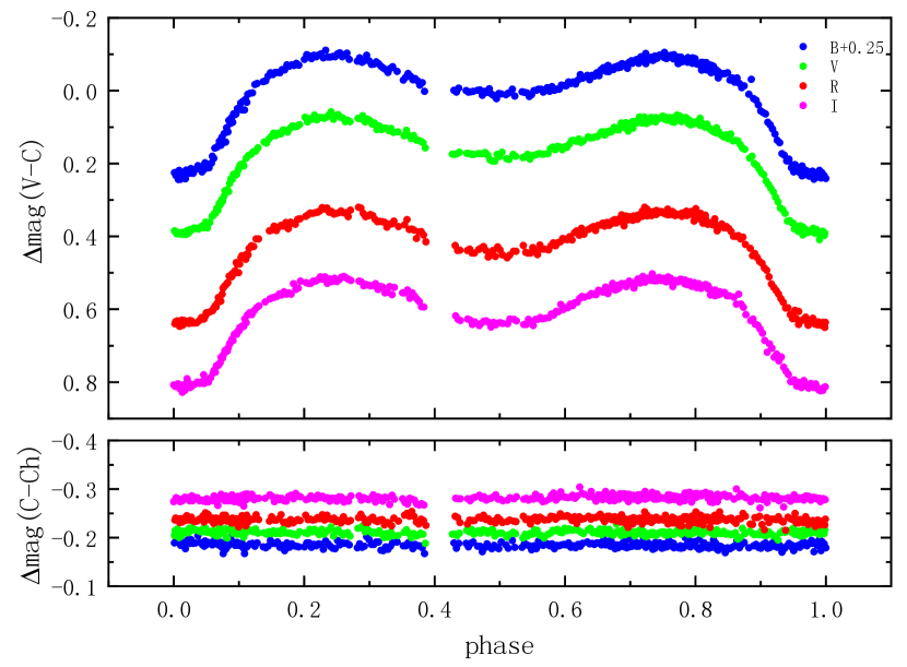
New photometric observations of the variable star CSS_J154915.7+375506 were carried out by the 1.5-m telescope AZT-22 on February 23, April 23, and June 23, 2023, at the Maidanak Astronomical Observatory (MAO) of the Ulugh Beg Astronomical Institute of the Uzbekistan Academy of Science (Ehgamberdiev, 2018). The optical system of the AZT-22 telescope is Ritchey-Chretien, and the focal length is 11560 mm (Artamonov, 1998). The Andor iKon-XL (XL-EA07-DS) ( $4096(H)\times 4108(V)$ ) CCD camera was used as the receiver. The read-out noise and amplification coefficients of the CCD camera are 6.5ADUs and 1.55 e-, the effective field of view is $18.1^{\prime}\times 18.1^{\prime}$ arcmin, and the pixel scale is 0.268^′ arcsec per pixel. In combination with the CCD detector, these provided a photometric system close to the standard Bessell UBVRI system (Im et al., 2010). Image acquisition was done with MaxIm DL 6 version. The observations were using the BVRI filters of the Bessell photometric system at 30, 20, 10 and 10 second exposure times, respectively. Figure 1 shows the EB multicolor light curves, and the standard deviation of the comparison minus the check are 0.00683, 0.00524, 0.00622 and 0.00582 for B, V, R and I, respectively. The coordinates of the comparison and check stars are listed in Table 1. In the light curves, the difference between the primary minimum and the secondary is close to 0.2 mag, with the flat primary minimum, this system should be a total eclipse binary.

Table 1: The coordinates of CSS_J154915.7+375506, the comparison star and the check star.

Stars	$\alpha_{2000}$	$\delta_{2000}$
CSS_J154915.7+375506	$15^{h}49^{m}15^{s}.76$	$+37^{\circ}55^{\prime\prime}06^{\prime}.01$
The comparison	$15^{h}49^{m}08^{s}.88$	$+37^{\circ}50^{\prime\prime}21^{\prime}.19$
The check	$15^{h}49^{m}09^{s}.79$	$+37^{\circ}55^{\prime\prime}18^{\prime}.64$

Refer to caption — Figure 1: The light curves of CSS_J154915.7+375506 in the Bessell B, V, $R$ and $I$ bands were observed by the 1.5 m AZT-22 telescope. The magnitude difference of the comparison star minus the check star (C-Ch) is shown in the bottom panel.

2.2 LAMOST Spectrum

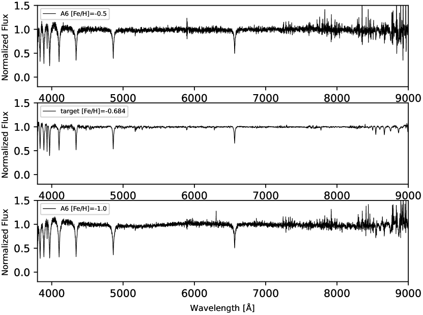
LAMOST is a reflective Schmidt telescope with a 4-meter aperture and a 5-degree field of view, which is located at the Xinglong Observatory in Hebei, China. With 4000 fibers placed on the focal plane, LAMOST can obtain 4000 spectra simultaneously. Meanwhile, stellar atmospheric parameters can be obtained automatically by the LAMOST stellar parameter pipeline (LASP) (Wu et al., 2011, 2014; Luo et al., 2015). The low-resolution spectrum of LAMOST is $R~{}1800$ and the wavelength range is 3700-9100Å. We found one low-resolution spectrum from the LAMOST DATA RELEASE 9 and obtained the atmospheric parameters as spectral type: A6, surface effective temperature: $6929.51\,K$ , surface gravity: $4.259\,dex$ and the metallicity: -0.684. The normalized spectrum is shown in Figure 2, in which located in the upper panel and lower panel are A6 type spectral template(Kesseli et al., 2017) for comparison.

3 Light curve Analysis

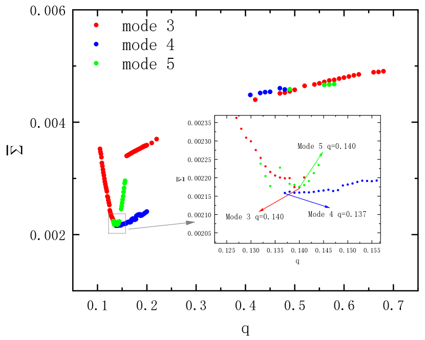
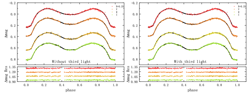
The Wilson-Devinney(Wilson & Devinney, 1971; Wilson, 1990, 2012; Wilson & Hamme, 2013) code was applied to analyze the multicolor light curves. The surface effective temperature of the primary component was set to $T_{1}$ = 6930 K according to the stellar atmospheric parameters of LAMOST. The gravity-darkening coefficients $g_{1}$ = 0.32 and $g_{2}$ = 0.32(Lucy, 1967), the bolometric albedo $A_{1}$ = 0.5 and $A_{2}$ = 0.5 (Rucinski, 1969) were adopted. We tried to adopt mode 2 (detached binary), mode 3 (overcontact binary), mode 4 (semidetached binary with star 1 nearly filling its Roche lobe) and mode 5 (semidetached binary with star 2 nearly filling its Roche lobe) to fit the light curves but mode 2 failed to converge. We used the q-search method to derive initial mass ratio. For mode 3, 4 and 5, convergent solutions were obtained when the mass ratio was fixed as a series of values from 0.1 to 1 with a step of 0.001. The minimum values of $\Sigma$ were achieved at similar q values: 0.140, 0.137 and 0.140, respectively, which indicates the reliability of the mass ratio. The q-search diagram is shown in Figure 3. After that, we set the q with the value 0.137 and rerun to run the WD code for the three modes. The other adjustable parameters of mode 3 are the orbital inclination, $i$ , the mean surface temperature of the secondary component, $T_{2}$ , the dimensionless potential of the primary, $\Omega_{1}$ (with $\Omega_{2}=\Omega_{1}$ ), the band-pass luminosity of the primary, $L_{1}$ , and the third light, $L_{3}$ . For mode 4, the only difference with mode 3 is the adjustable dimensionless surface potential is of the secondary, $\Omega_{2}$ . As for mode 5, the adjustable parameters are the same as that of mode 3 (with $\Omega_{1}\neq\Omega_{2}$ ). All the convergent solutions are listed in Table 2. The $\Sigma$ can be noticed in the last row of the table, and no large difference exists; as an example, the fitted light curves of mode 3 with and without $L_{3}$ are shown in Figure 4. It can be seen from Figure 4 that the fits with $L_{3}$ look almost identical to the fits without $L_{3}$ but smaller residuals can be noticed from the Table 2. So CSS_J154915.7+375506 may be a marginal contact binary with an extremely low mass ratio, with the low contribution of third light, a faint third companion could exist.

Table 2: Photometric solutions of CSS_J154915.7+375506 obtained by using the W-D code. The units of most parameters are dimensionless, except those already mentioned.

Parameters	Without $L_{3}$	With $L_{3}$	Without $L_{3}$	With $L_{3}$	Without $L_{3}$	With $L_{3}$
	Mode 3		Mode 4		Mode 5
$g_{1}=g_{2}$	0.32	0.32	0.32	0.32	0.32	0.32
$A_{1}=A_{2}$	0.5	0.5	0.5	0.5	0.5	0.5
$q(M_{2}/M_{1})$	0.13875(55)	0.13824(91)	0.13828(46)	0.13828(89)	0.13729(28)	0.13696(61)
$i(^{\circ})$	86.153(97)	86.151(97)	85.796(95)	85.796(98)	87.17(12)	87.02(11)
$T_{1}(K)$	6930	6930	6930	6930	6930	6930
$T_{2}(K)$	4209(33)	4210(33)	4184(30)	4184(31)	4225(30)	4223(32)
$\Omega_{1}$	2.0720(22)	2.0706(24)	2.07088	2.07088	2.07093(36)	2.07007(43)
$\Omega_{2}$	2.0720(22)	2.0706(24)	2.0714(21)	2.0714(21)	2.06814	2.06722
$L_{1}/(L_{1}+L_{2})_{B}$	0.9951413(26)	0.995146(35)	0.9954392(21)	0.995439(39)	0.9949932(25)	0.995026(22)
$L_{1}/(L_{1}+L_{2})_{V}$	0.9892739(82)	0.989289(86)	0.9898197(72)	0.989820(97)	0.9890236(81)	0.989085(59)
$L_{1}/(L_{1}+L_{2})_{R}$	0.982783(16)	0.98281(15)	0.983541(15)	0.98354(17)	0.982461(16)	0.98255(11)
$L_{1}/(L_{1}+L_{2})_{I}$	0.974829(26)	0.97488(24)	0.975723(25)	0.97572(27)	0.974491(26)	0.97460(18)
$L_{3}/(L_{1}+L_{2}+L_{3})_{B}$	–	0.0131(65)	–	0.0126(75)	–	0.0113(42)
$L_{3}/(L_{1}+L_{2}+L_{3})_{V}$	–	0.010711(86)	–	0.0018(86)	–	0.0003(51)
$L_{3}/(L_{1}+L_{2}+L_{3})_{R}$	–	0.00048(838)	–	0.0011(93)	–	0.0000(61)
$L_{3}/(L_{1}+L_{2}+L_{3})_{I}$	–	$9.4\times 10^{-5}(9.2\times 10^{-3})$	–	0.0019(102)	–	0.0000(70)
$r_{1}(pole)$	0.51311(44)	0.51329(45)	0.51338(23)	0.51328(44)	0.51316(10)	0.51328(16)
$r_{1}(side)$	0.56504(64)	0.5653(065)	0.56543(32)	0.56529(62)	0.56505(16)	0.56521(27)
$r_{1}(back)$	0.58524(67)	0.58551(67)	0.58566(3)	0.58552(57)	0.58504(21)	0.58518(40)
$r_{2}(pole)$	0.2175(21)	0.2176(3)	0.2172(18)	0.2175(27)	0.21698(13)	0.21684(28)
$r_{2}(side)$	0.2092(18)	0.2093(25)	0.209(16)	0.2092(23)	0.20869(13)	0.20856(27)
$r_{2}(back)$	0.2492(40)	0.2495(58)	0.2488(35)	0.2492(53)	0.24868(14)	0.24853(29)
$fill-outfactor$	0.00231(0.02415)	0.00228(0.026452)	–	–	–	–
$\Sigma$	0.00204	0.00169	0.00203	0.00169	0.00203	0.00170

4 Orbital Period Investigation

Table 3: The light minima of CSS_J154915.7+375506.

Eclipse timings	Error	E	O-C	Reference
(HJD)	( $\pm$ d)		(d)
2457208.72	0.001432612	0	0.00000000	ASAS-SN
2458005.934	0.001436392	2109	0.01637465	ASAS-SN
2454143.537	0.000506517	-8109	0.00223421	CRTS
2455615.454	0.000971455	-4215	-0.00444866	CRTS
2458269.408	0.000374218	2806	0.02509633	ZTF
2458630.022	0.000442258	3760	0.02942852	ZTF
2459015.204	0.000351538	4779	0.03178869	ZTF
2459363.34	0.000408238	5700	0.03150496	ZTF
2459743.98	0.000782456	6707	0.0274099	ZTF
2460161.285	0.0002675	7811	0.02224803	AZT-22
2458962.284	0.000287278	4639	0.03109575	TESS s24
2458975.892	0.000238139	4675	0.03143317	TESS s24
2459669.139	0.000487617	6509	0.03005764	TESS s50
2459675.565	0.000449818	6526	0.03010509	TESS s50
2459682.747	0.000540537	6545	0.0295658	TESS s50
2459688.795	0.000389338	6561	0.0295849	TESS s50
2459695.976	0.000287278	6580	0.02904642	TESS s51
2459702.024	0.000241919	6596	0.02900456	TESS s51
2459708.828	0.000351538	6614	0.02884077	TESS s51
2459714.876	0.000268379	6630	0.02880401	TESS s51

Table 4: Orbital parameters of the third body in CSS_J154915.7+375506.

Parameter	Value	Unit
Case A: linear term plus
cyclical variation( $\beta=0$ )
Revised epoch, $T_{0}$	2457208.7277( $\pm$ 0.0007)	HJD
Revised period, $P_{0}$	0.37800020( $\pm$ 0.00000010)	days
Eccentricity, $e_{3}$	0 (assumed)	–
Long-term change of the orb-
ital period, $\beta$	0 (assumed)	d cycle^-1
Orbital period, $P_{3}$	12.48( $\pm$ 0.25)	yr
Amplitude, A	0.0142( $\pm$ 0.0006)	days
Projected semi-major axis, $a_{12}sin(i_{3})$	2.45( $\pm$ 0.10)	au
Mass function, $f(m)$	0.10( $\pm$ 0.01)	$M_{\odot}$
Mass, $M_{3min}$	1.02( $\pm$ 0.05)	$M_{\odot}$
Sum of the squares of the residuals, $\Sigma$	$1.66\times 10^{-5}$	–
Case B: quadratic term plus
cyclical variation( $\beta\neq 0$ )
Revised epoch, $T_{0}$	2457208.7335( $\pm$ 0.0017)	HJD
Revised period, $P_{0}$	0.37798160( $\pm$ 0.00000030)	days
Eccentricity, $e_{3}$	0 (assumed)	–
Long-term change of the orb-
ital period, $\beta$	$-3.25(\pm 0.89)\times 10^{-10}$	d cycle^-1
Orbital period, $P_{3}$	14.89( $\pm$ 0.96)	yr
Amplitude, A	0.0145( $\pm$ 0.0010)	days
Projected semi-major axis, $a_{12}sin(i_{3})$	2.51( $\pm$ 0.17)	au
Mass function, $f(m)$	0.07( $\pm$ 0.02)	$M_{\odot}$
Mass, $M_{3min}$	0.91( $\pm$ 0.06)	$M_{\odot}$
Sum of the squares of the residuals, $\Sigma$	$2.98\times 10^{-5}$	–
Case C: linear term plus
eccentric orbit( $\beta=0$ )
Revised epoch, $T_{0}$	2457208.7237( $\pm$ 0.0030)	HJD
Revised period, $P_{0}$	0.37800028( $\pm$ 0.00000005)	days
Eccentricity, $e_{3}$	0.40( $\pm$ 0.15)	–
Long-term change of the orb-
ital period, $\beta$	0 (assumed)	d cycle^-1
Orbital period, $P_{3}$	12.37( $\pm$ 0.11)	yr
Amplitude, A	0.0175( $\pm$ 0.0029)	days
Longitude of the periastron
passage, $\omega_{3}$	260.02( $\pm$ 8.85)	degree
Time of periastron passage, $T_{3}$	2456409.0183( $\pm$ 120.5700)	days
Projected semi-major axis, $a_{12}sin(i_{3})$	3.03( $\pm$ 0.50)	au
Mass function, $f(m)$	0.18( $\pm$ 0.09)	$M_{\odot}$
Mass, $M_{3min}$	1.36( $\pm$ 0.19)	$M_{\odot}$
Sum of the squares of the residuals, $\Sigma$	$1.73\times 10^{-5}$	–

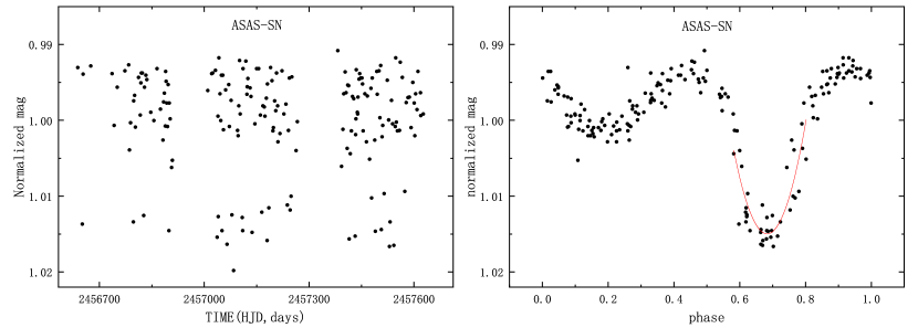
Orbital period variations are common in binary systems which are usually caused by angular momentum loss, mass transfer, third body or magnetic activity. We used the O-C method to analyze the orbital period variation of this system. To obtain more light minimum times, we tried to search for more photometric data from the sky survey project and public databases. We collected data from All-Sky Automated Survey for Supernovae (ASAS-SN)(Shappee et al., 2014; Christy et al., 2023) database, Catalina Real-Time Transient Survey (CRTS)(Drake et al., 2009) database, The Zwicky Transient Facility (ZTF)(Bellm et al., 2018) and Transiting Exoplanet Survey Satellite (TESS) (Ricker et al., 2010) which provided Full Frame Images (FFI) for three sectors with an exposure time of the 1800s, 600s and 600s. We converted data with more than one cycle into a phase (Shi et al., 2021; Li et al., 2022) to get the minima by using parabola fitting. Some data of the ASAS-SN is shown in the left panel of Figure. 5 and the right panel shows the light curve converted to one phase. Finally, we obtained 2 times of minimum from ASAS-SN, 2 times of minimum from CRTS, 5 times of minimum from ZTF and 10 times of minimum from TESS, plus the 1 fitted from AZT-22 data, 20 in total. The times of light minima are listed in the first column of the Table. 3. The $O-C$ values were calculated with the following linear ephemeris formula:

Min.I(HJD)=2457208.72017397+0^{d}.377998\times E

(1)

In which the $HJD_{0}$ and period value was obtained from The International Variable Star Index(VSX)¹¹1https://www.aavso.org/vsx/. In O-C curves, it is clear that a periodic oscillation exists which may be caused by the light time travel effect(LTTE) of a third body(Liao & Qian, 2010). We use the following general equation to fit the O-C diagram(Irwin, 1952):

$\displaystyle O-C$	$\displaystyle=\Delta T_{0}+\Delta P_{0}E+\frac{\beta}{2}E^{2}$	(2)
	$\displaystyle\phantom{{}={}}+A[(1-e^{2}_{3})\frac{sin(\nu+\omega)}{1+e_{3}cos\nu}+esin\omega]$
	$\displaystyle=\Delta T_{0}+\Delta p_{0}E+\frac{\beta}{2}E^{2}$
	$\displaystyle\phantom{{}={}}+A[\sqrt{1-e_{3}^{2}}sinE^{}cos\omega+cosE^{}sin\omega]$

The Kepler equation is as follows:

M=E^{*}-e_{3}sinE^{*}=\frac{2\pi}{P_{3}}(t-T_{3})

(3)

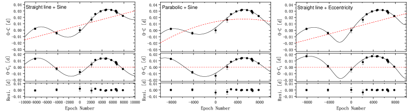
the meaning of each parameter is described very clearly in the paper (Liao et al., 2021). The corresponding results of Equations2 and 3 are displayed in Table 4. Based on the existence of the periodic oscillation, we assumed a circular orbit( $e_{3}=0$ ), i.e. (1) Case A, the linear term plus cyclical variation( $\beta=0$ ) and (2) Case B, the quadratic term plus cyclical variation( $\beta\neq 0$ ). In addition, we considered an eccentric orbit ( $e_{3}\neq 0$ ) with a linear term, i.e. (3) Case C, the linear term plus eccentric orbit( $\beta=0$ ). By using Equation 2 and 3 to fit the O-C cure, the results of the three cases are listed in Table 4. The fitted O-C curve and the residuals for different cases are shown in Figure 6. For Case A, the amplitude and period of the cyclical variation are $A=0.0142(\pm 0.0006)\,days$ and $P_{3}=12.48(\pm 0.25)\,yr$ . For Case B, the amplitude and period of the cyclical variation are $0.0145(\pm 0.0010)\,days$ and $P_{3}=14.89(\pm 0.96)\,yr$ with a long-term period decrease at a rate: $\beta=-3.25\times 10^{-10}\,d\,cycle^{-1}$ , i.e. $-3.14(\pm 0.89)\times 10^{-7}\,days\,yr^{-1}$ . We can see different possible O-C curve variations correspond to different cases, but a common periodic oscillation may imply an existence of a third body, so further investigations are necessary. As for the Case C, the eccentricity of the third body is $e_{3}=0.40(\pm 0.15)$ , the amplitude and period of the cyclical variation are $A=0.0175(\pm 0.0029)\,days$ and $P_{3}=12.37(\pm 0.11)\,yr$ , respectively.

5 Discussion and Conclusion

5.1 Absolute parameters

Table 5: Estimated absolute parameters of CSS_J154915.7+375506

Parameters	Value	Parameters	Value
$\varpi$ (mas)	0.6934(0.014)	$A_{v}$	0.035
$m_{V}$	13.776(0.023)	$M_{v}$	2.95(0.05)
$M_{bol}$	2.88(0.05)	$BC_{V}$	-0.07
$M_{1}$	2.05(0.15)	$M_{2}$	0.283(0.02)
$R_{1}$	1.62(0.04)	$R_{2}$	0.656(0.016)
$L_{1}$	5.43(0.27)	$L_{2}$	0.121(0.006)
semi major axis	2.92(0.07)

The orbital period analysis and multicolor CCD photometric solutions of CSS_J154915.7+375506 are presented for the first time. With the newly observed multicolor light curves, good photometric solutions on mode 3, mode 4 and mode 5 were obtained by using W-D code. Although the radial velocity curve is missing, it is a total eclipse binary system, and all solutions show similar mass ratios, so the results are reliable. The solutions are shown to us in Table 2 that all the convergent solutions are with very close parameter values and similar residuals, and all solutions with $L_{3}$ have smaller residuals, so we will take the average values of the results with $L_{3}$ for the following discussions.

Combined with the photometric solutions and parallax, the absolute parameters can be estimated by the method described by (Li et al., 2021) and (Xu et al., 2022). The parallax $\varpi$ was given by Gaia Dr3 as 0.6934 mas, so the distance was estimated as about 1442 pc, which was calculated by the following formula:

(m-M)_{v}=10-5lg\varpi+A_{v}

(4)

where the extinction $A_{v}$ is 0.035 mag (obtained from the NASA/IPAC Extragalactic Database²²2https://ned.ipac.caltech.edu/extinction_calculator.), and the apparent magnitude $m_{v}$ is 13.776 mag, the maximum brightness in the V band from ASAS-SN data(Shappee et al., 2014; Christy et al., 2023). Then with the bolometric correction $BC_{v}=$ -0.07 mag(Worthey & Lee, 2011), we can obtain its bolometric absolute magnitude $M_{v}$ with this equation:

M_{bol}=M_{v}+BC_{v}

(5)

hence, the total luminosity $L_{t}$ of the binary system is derived by:

L_{T}=L_{1}+L_{2}=10^{(M_{bol}-4.74)/-2.5}

(6)

And with the Stefan Boltzmann’s law, we have:

L_{t}/L_{\odot}=(ar_{1})^{2}\times(\frac{T_{1}}{T_{\odot}})^{4}+(ar_{2})^{2}\times(\frac{T_{2}}{T_{\odot}})^{4}

(7)

where $T_{\odot}$ represents the effective temperature of the sun, with a value of 5772 K. $r_{1}$ and $r_{2}$ represent the relative radii of the star 1 and star 2, respectively, which can be obtained from the photometric solutions, just like $r_{i}=(r_{ipole}*r_{iside}*r_{iback})^{1/3}$ . The semi-major axis $a$ is obtained as about $2.92\,R_{\odot}$ . Combined with the mass ratio and the Kepler’s third law,

\frac{a^{3}}{P^{2}}=74.5(M_{1}+M_{2}),

(8)

q=\frac{M_{2}}{M_{1}}

(9)

the mass of the primary component $M_{1}$ and the mass of the secondary component $M_{2}$ were calculated about 2.05 $M_{\odot}$ and 0.283 $M_{\odot}$ , respectively. All the estimated absolute parameters are tabulated in Table 5.

5.2 Orbital period variations

In the present paper, the orbital period changes are studied for the first time by analyzing a total of 20 times of minima with time span of 16 years. In Case B, a long-term period decrease and periodic oscillation are revealed with $\beta=-3.14(\pm 0.89)\times 10^{-7}\,days\,yr^{-1}$ . According to the period variation equation:

\frac{\dot{P}}{P}=-3(\frac{\dot{M_{1}}}{M_{1}}+\frac{\dot{M_{2}}}{M_{2}}),

(10)

we can get the rate of mass transfer from the primary to the secondary is $\dot{M_{1}}=-9.1(\pm 2.8)\times 10^{-8}M_{\odot}\,yr^{-1}$ . Without more long-term observations, we cannot determine whether the period decrease exists or not. In general, all cases of O-C curve analysis show evidences of the periodic oscillation. Considering that the target is an A-type marginal contact binary and photometric solutions with third lights from symmetrical light curves were obtained, the oscillations are mostly caused by the LTTE of a third body. In order to do further study on the period variation, we use the following formula to estimate the possible parameters of the third body:

f(m)=\frac{(M_{3}sini_{3})^{3}}{(M_{1}+M_{2}+M_{3})^{2}}=\frac{4\pi^{2}}{GP_{3}^{2}}\times(a_{12}sini_{3})^{3},

(11)

the mass function of this system is $f(m)=0.10(\pm 0.01)\,M_{\odot}$ for Case A, $f(m)=0.07(\pm 0.02)\,M_{\odot}$ for Case B and $f(m)=0.18(\pm 0.09)\,M_{\odot}$ for Case C. By assuming the orbital inclination $i_{3}=90^{\circ}$ , we can estimate the minimum mass of the third body are $M_{3}=1.02(\pm 0.05)\,M_{\odot}$ , $M_{3}=0.91(\pm 0.06)\,M_{\odot}$ and $M_{3}=1.36(\pm 0.19)\,M_{\odot}$ respectively. However, considering the extremely low contribution of the third light, this third body may be not in its main-sequence stage, perhaps an unseen compact object. Some statistics indicate that third bodies are common in contact binaries(Tokovinin et al., 2006; Pribulla & Rucinski, 2006; D’Angelo et al., 2006; Rucinski et al., 2007), and the existence of a third body may play an important role in the binary’s evolution. Core fragmentation is thought to be the way to form binary system(Boss, 1986; Bate et al., 1995). However, binaries yielded by this mechanism correspond to initial separations range of 10 to 1000 au. One way of forming closer binaries is dynamical interactions with other nearby stars(Bate et al., 2002). Dynamical interactions often result in the replacement of the lower-mass binary component with a higher-mass third body. Consequently, the original system undergoes a process where the lower-mass component is ejected to a wider orbit, forming a hierarchical triple system. Through the passage of time, these processes have a tendency to give rise to binary systems featuring closely spaced components and almost equivalent masses(Bate et al., 2002; Gullikson & Dodson-Robinson, 2013). Based on our system, the mass of the third body is greater than that of the secondary component, indicating that CSS_J154915.7+375506 is the original one and was not replaced by the third body. Therefore, the third carried some dynamical characteristics during binary star formation.

5.3 Discussion

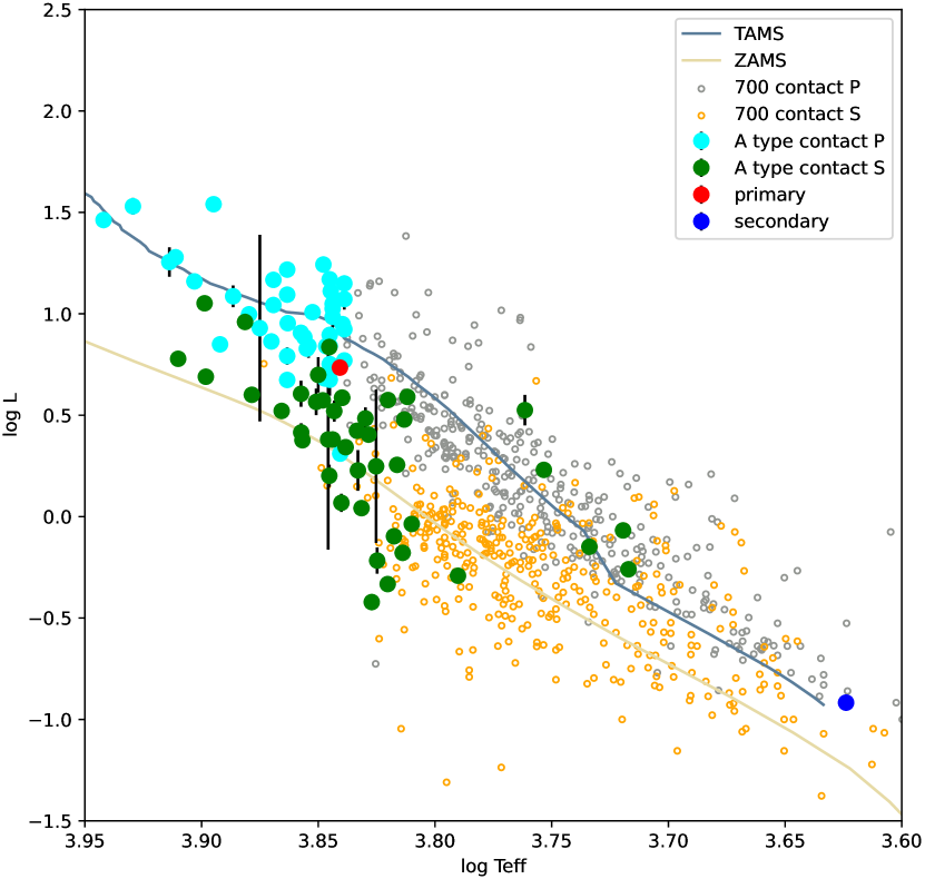
Hertzsprung-Russell diagram with [Fe/H] = -0.75 was displayed in Figure 7. The primary and secondary of this system are plotted in this figure. Besides, we plotted 700 contact binaries(Latković et al., 2021) and selected spectral A type contact binaries by setting the primary temperature range $6900\,K<T_{1}<9000\,K$ . From this diagram, normal contact binaries’ primary components are usually more evolved, while the secondary is not. As for A type contact binaries, most of the primaries are evolved to near the TAMS(terminal-age main-sequence), and the secondaries just went through the ZAMS(zero-age main-sequence) (Dotter, 2016; Choi et al., 2016). CSS_J154915.7+375506 is different, the primary component is in main-sequence near the TAMS, while the secondary seems to just deviate from the TAMS. Under this situation: the extremely low mass ratio of 0.138 with the mass of the secondary of $0.283\,M_{\odot}$ , which is much less than the primary component. The secondary should not have evolved so quickly on its own(Clayton, 1983; Paczyński, 1971), so it must be caused by the interaction between the two components.

Now let’s consider the aspect of mutual influence between the binary components. On the one hand, the secondary star has a much smaller mass than the primary star, but it is more evolved, indicating that the secondary star was once the primary star. It evolved faster and transferred a large amount of mass to the current primary star(Crawford, 1955). Its characteristic of marginal contact indicates that this system has just experienced a mass ratio reversal and is evolving towards the next stage.

On the other hand, the current photometric solutions indicate that the mass of the secondary star is $0.283\,M_{\odot}$ , but the temperature is higher than 4000 K. This suggests that the secondary star, after evolving and expanding, has shed its outer material and exposed part of its core, which is why its current temperature is relatively high. According to the O-C curve analysis, if the long-term period decreasing really exists, the system will evolve to be a contact binary.

5.4 Conclusion

In conclusion, the distinct characteristics of CSS_J154915.7+375506, including its exceptionally low mass ratio and the evolutionary status of its secondary component, together with its high temperature relative to its mass, suggest that the system has undergone significant mass transfer, likely experienced a mass ratio reversal event. Furthermore, considering the evidence from current photometric solutions and the potential for long-term period decrease based on O-C curve analysis, the system may evolve towards becoming a contact binary. Therefore, CSS_J154915.7+375506 serves as an intriguing subject for investigating the formation processes and evolutionary pathways of binary systems.

6 DATA AVAILABILITY

The data underlying this article will be uploaded to the VizieR data base (CDS).

Acknowledgements

This work is supported by the International Cooperation Projects of the National Key R&D Program (No. 2022YFE0127300), the Science Foundation of Yunnan Province (No. 202401AS070046), the National Natural Science Foundation of China (Nos. 11933008 and 11922306), the Agency of innovative development under the Ministry of higher education, science and innovation of the Republic of Uzbekistan. Project (AL-5921122128): "Investigations and observations of special LAMOST eclipsing binaries based on telescopes in Uzbekistan and China", CAS "Light of West China" Program and Yunnan Revitalization Talent Support Program.The new CCD photometric data were obtained with the Maidanak Astronomical Observatory 1.5 m telescope. This work has made use of data from the All-Sky Automated Survey for Supernovae (ASAS-SN), Catalina Real-Time Transient Survey (CRTS), The Zwicky Transient Facility (ZTF), the Large-Sky-Area Multi-Object Fiber Spectroscopic Telescope (LAMOST), the Transiting Exoplanet Survey Satellite (TESS), and Gaia and the authors thank the teams for providing open data.

References

Artamonov (1998) Artamonov B., 1998, in Symposium-International Astronomical Union. pp 121–122
Bate et al. (1995) Bate M. R., Bonnell I. A., Price N. M., 1995, MNRAS, 277, 362
Bate et al. (2002) Bate M. R., Bonnell I. A., Bromm V., 2002, MNRAS, 336, 705
Bellm et al. (2018) Bellm E. C., et al., 2018, Publications of the Astronomical Society of the Pacific, 131, 018002
Boss (1986) Boss A. P., 1986, ApJS, 62, 519
Choi et al. (2016) Choi J., Dotter A., Conroy C., Cantiello M., Paxton B., Johnson B. D., 2016, ApJ, 823, 102
Christy et al. (2023) Christy C. T., et al., 2023, MNRAS, 519, 5271
Clayton (1983) Clayton D. D., 1983, Principles of stellar evolution and nucleosynthesis. University of Chicago press
Crawford (1955) Crawford J., 1955, Astrophysical Journal, vol. 121, p. 71, 121, 71
D’Angelo et al. (2006) D’Angelo C., van Kerkwijk M. H., Rucinski S. M., 2006, AJ, 132, 650
Dotter (2016) Dotter A., 2016, ApJS, 222, 8
Drake et al. (2009) Drake A. J., et al., 2009, ApJ, 696, 870
Drake et al. (2014) Drake A. J., et al., 2014, The Astrophysical Journal Supplement Series, 213, 9
Ehgamberdiev (2018) Ehgamberdiev S., 2018, Nature Astronomy, 2, 349
Flannery (1976) Flannery B. P., 1976, The Astrophysical Journal, 205, 217
Gullikson & Dodson-Robinson (2013) Gullikson K., Dodson-Robinson S., 2013, AJ, 145, 3
Im et al. (2010) Im M.-S., Ko J.-W., Cho Y.-S., Choi C.-S., Jeon Y.-S., Lee I.-D., Ibrahimov M., 2010, Journal of Korean Astronomical Society, 43, 75
Irwin (1952) Irwin J. B., 1952, The Astrophysical Journal, 116, 211
Kesseli et al. (2017) Kesseli A. Y., West A. A., Veyette M., Harrison B., Feldman D., Bochanski J. J., 2017, ApJS, 230, 16
Latković et al. (2021) Latković O., Čeki A., Lazarević S., 2021, ApJS, 254, 10
Li et al. (2021) Li K., et al., 2021, AJ, 162, 13
Li et al. (2022) Li F. X., Liao W. P., Qian S. B., Fernández Lajús E., Zhang J., Zhao E. G., 2022, ApJ, 924, 30
Liao & Qian (2010) Liao W.-P., Qian S.-B., 2010, Monthly Notices of the Royal Astronomical Society, 405, 1930
Liao et al. (2021) Liao W., Qian S., Li L., 2021, Monthly Notices of the Royal Astronomical Society, 508, 6111
Lucy (1967) Lucy L. B., 1967, Z. Astrophys., 65, 89
Lucy (1976a) Lucy L. B., 1976a, ApJ. . ., 205
Lucy (1976b) Lucy L. B., 1976b, ApJ, 205, 208
Lucy & Wilson (1979) Lucy L. B., Wilson R. E., 1979, The Astrophysical Journal, 231, 502
Luo et al. (2012) Luo A. L., et al., 2012, Research in Astronomy and Astrophysics, 12, 1243
Luo et al. (2015) Luo A.-L., et al., 2015, Research in Astronomy and Astrophysics, 15, 1095
Marsh et al. (2017) Marsh F. M., Prince T. A., Mahabal A. A., Bellm E. C., Drake A. J., Djorgovski S. G., 2017, MNRAS, 465, 4678
Paczyński (1971) Paczyński B., 1971, ARA&A, 9, 183
Pribulla & Rucinski (2006) Pribulla T., Rucinski S. M., 2006, AJ, 131, 2986
Ricker et al. (2010) Ricker G. R., et al., 2010, in American Astronomical Society Meeting Abstracts# 215. pp 450–06
Rucinski (1969) Rucinski S., 1969, Acta Astronomica, Vol. 19, p. 245, 19, 245
Rucinski et al. (2007) Rucinski S. M., Pribulla T., van Kerkwijk M. H., 2007, AJ, 134, 2353
Shappee et al. (2014) Shappee B. J., et al., 2014, ApJ, 788, 48
Shaw et al. (1994) Shaw J. S., Caillault J. P., Schmitt J. H. M. M., 1994, in American Astronomical Society Meeting Abstracts. p. 85.06
Shi et al. (2021) Shi X.-d., Qian S.-b., Li L.-j., Liao W.-p., 2021, Monthly Notices of the Royal Astronomical Society, 505, 6166
Skarka et al. (2017) Skarka M., et al., 2017, Open European Journal on Variable Stars, 185, 1
Stępień & Kiraga (2013) Stępień K., Kiraga M., 2013, Acta Astron., 63, 239
Tokovinin et al. (2006) Tokovinin A., Thomas S., Sterzik M., Udry S., 2006, A&A, 450, 681
Wilson (1990) Wilson R. E., 1990, ApJ, 356, 613
Wilson (2012) Wilson R. E., 2012, The Astronomical Journal, 144, 73
Wilson & Devinney (1971) Wilson R. E., Devinney E. J., 1971, ApJ, 166, 605
Wilson & Hamme (2013) Wilson R. E., Hamme W. V., 2013, The Astrophysical Journal, 780, 151
Worthey & Lee (2011) Worthey G., Lee H. C., 2011, VizieR Online Data Catalog, p. J/ApJS/193/1
Wu et al. (2011) Wu Y., et al., 2011, Research in Astronomy and Astrophysics, 11, 924
Wu et al. (2014) Wu Y., Du B., Luo A., Zhao Y., Yuan H., 2014, Proceedings of the International Astronomical Union, 10, 340
Xu et al. (2022) Xu H.-S., Zhu L.-Y., Thawicharat S., Boonrucksar S., 2022, Research in Astronomy and Astrophysics, 22, 035024
Zhao et al. (2012) Zhao G., Zhao Y.-H., Chu Y.-Q., Jing Y.-P., Deng L.-C., 2012, Research in Astronomy and Astrophysics, 12, 723
Zhu & Qian (2006) Zhu L., Qian S., 2006, MNRAS, 367, 423
Zhu & Qian (2009) Zhu L., Qian S., 2009, in Murphy S. J., Bessell M. S., eds, Astronomical Society of the Pacific Conference Series Vol. 404, The Eighth Pacific Rim Conference on Stellar Astrophysics: A Tribute to Kam-Ching Leung. p. 189