Curvature Fields, Topology, and the Dynamics of Spatiotemporal Chaos

When a system governed by nonlinear equations of motion is driven out of equilibrium, a variety of complex behaviors can result, ranging from chaos in low-dimensional systems Ott (1981) to the seemingly random dynamics of turbulent flows Falkovich et al. (2001). If the number of active degrees of freedom (roughly corresponding to the number of equations required to characterize the dynamics) is small, the mathematics of dynamical systems has proved to be a powerful tool. When it is quasi-infinite and the dynamics are turbulent, statistical approaches based on assumed scale invariance have been fruitful. For spatially-extended systems below the turbulence transition, however, a regime with a large but finite number of active degrees of freedom exists that is disordered both in space and in time Ciliberto and Bigazzi (1988); Rabaud et al. (1990); Shraiman et al. (1992); Cross and Hohenberg (1993); Dennin et al. (1996); Gollub and Langer (1999); Egolf et al. (2000). This regime of spatiotemporal chaos (STC) remains poorly characterized and understood; indeed, there is no generally agreed-upon quantitative indicator of STC.

In this Letter, we study the dynamics of a simple fluid flow that exhibits STC by considering its underlying topology. We describe a method for locating the time-dependent topologically special points of the flow, and show that their dynamics describe the flow pattern as a whole. These special points undergo pairwise interactions, changing the flow topology when they are created or annihilated. Surprisingly, we find that the rate of creation or annihilation shows a discrete onset, while other measures of spatial and temporal disorder increase smoothly with the rate of energy input. This form of STC is characterized not only by disorder but also by constantly changing flow topology.

In a driven body of fluid, there can exist instantaneous stagnation points where the velocity vanishes, relative to some observer. These special points carry the bulk of the information contained in the flow field: if the locations of all of these topologically special points and their local flow properties are known, most of the full flow field can be determined Perry and Chong (1987). They are also an essential component of chaotic mixing Jana and Ottino (1992). These points are distinct from the topological defects previously considered in studies of STC Egolf (1998); Daniels and Bodenschatz (2002); Young and Riecke (2003), as they are present even when the flow is not chaotic. In a two-dimensional (2D) flow field, the special points come in two types. When embedded in a region of the flow that is dominated by vorticity, they are elliptic; in a strain-dominated region, they are hyperbolic (i.e. saddle-like). These special points, however, have proved to be very difficult to identify, particularly in experimental flows. In this Letter, we show that by considering the curvature of Lagrangian trajectories, that is, the trajectories of individual moving fluid elements, we can find the elliptic and hyperbolic points in an automated way, even when they move. Once located, the trajectories and statistics of the special points give insight into the transition to and dynamics of STC.

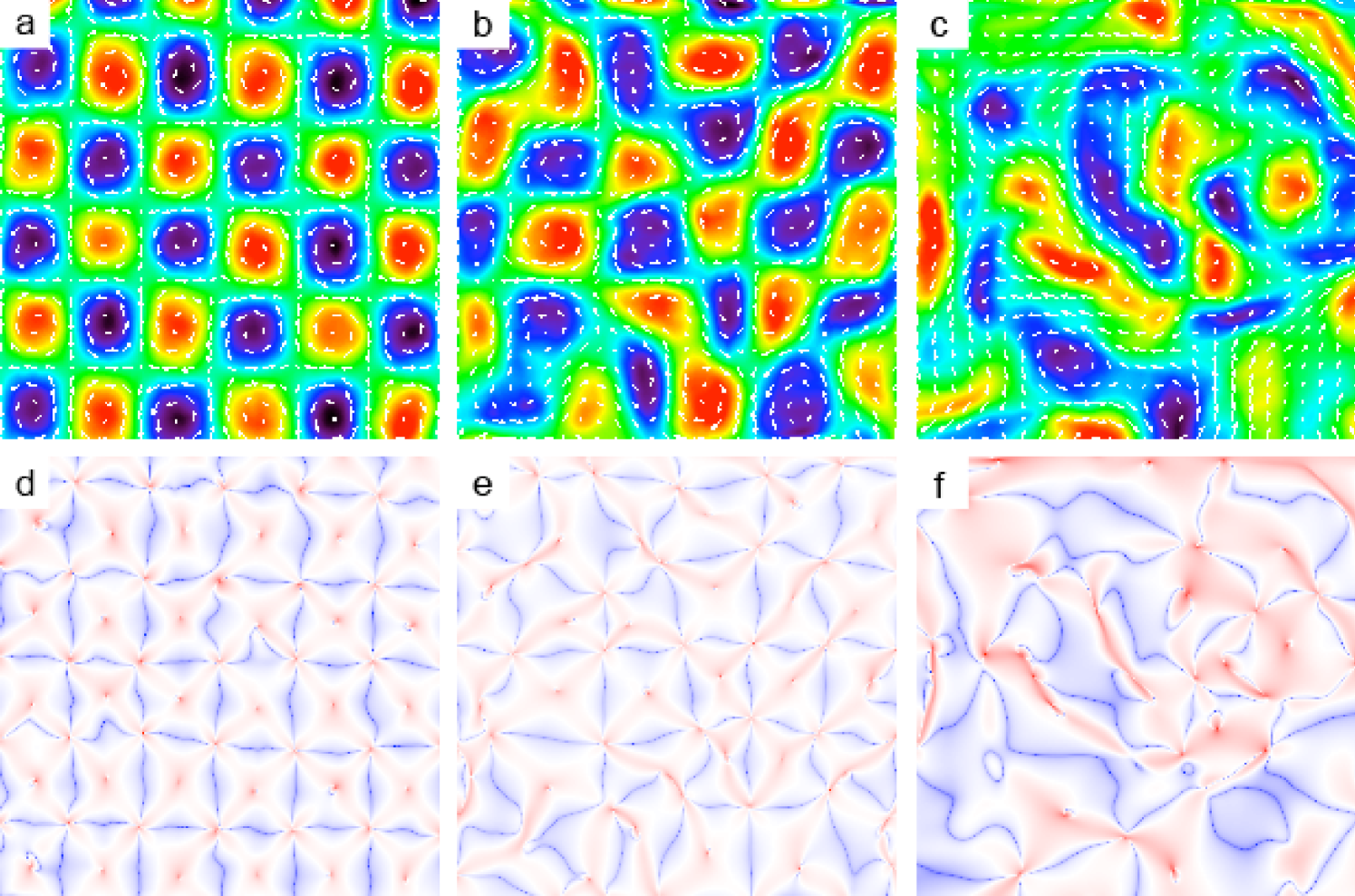
We generate a quasi-2D flow using magnetohydrodynamic forcing in a thin layer of conducting fluid, as described previously Rothstein et al. (1999); Paret et al. (1997). A 6 mm layer of water containing 8% by weight of CuSO₄ was placed above a square lattice of permanent magnets with alternating orientation. When a current is driven across the cell, Lorentz forces set the fluid into motion. The dimensionless strength of the forcing is measured by the Reynolds number $\mathrm{Re}=UL/\nu$, where $U$ is the root-mean-square velocity, $L=2$ cm is the mean magnet spacing, and $\nu$ is the kinematic viscosity. At low $\mathrm{Re}$, the flow is a square array of vortices of alternating sign, as shown in Fig. 1. As $\mathrm{Re}$ grows, however, the flow deviates from the forced lattice and becomes spatiotemporally chaotic. To measure the flow, we follow the simultaneous trajectories of thousands of neutrally-buoyant 116 $\mu$m fluorescent polystyrene tracer particles, using algorithms similar to those described by Ouellette et al. Ouellette et al. (2006). The particles are imaged at a rate of 12 Hz, and their positions are determined to a precision of 25 $\mu$m (0.1 pixels). The velocities and accelerations of the particles are then computed by fitting polynomials to short segments of the trajectories Voth et al. (2002). Statistics are collected in a 10 cm $\times$ 10 cm window in the center of the flow, so that boundary effects are excluded.

To find the elliptic and hyperbolic points, we first compute the curvature along the trajectories of the tracer particles. Curvature, a geometrical quantity containing, in principle, no dynamical information, completely specifies a curve in 2D space. Because of the nature of our measurement technique, however, the trajectories are parameterized by time. In this case, the Frenet formulas show that the curvature is given by $\kappa=a_{n}/u^{2}$, where $a_{n}$ is the acceleration normal to the direction of motion and $u$ is the velocity of the particle. The single-point statistics of curvature have previously been studied in turbulent flow Braun et al. (2006); Xu et al. (2007), but were found to be explainable with a simple model that should also apply to non-turbulent flows. In our flow, we measure curvature probability density functions (PDFs) that are consistent with the model proposed by Xu et al. Xu et al. (2007).

Instead of focusing on such single-point curvature statistics, we consider curvature fields, analogous to velocity or vorticity fields. Sample curvature fields for the steady and STC regimes are shown in Fig. 1, and striking structure is evident. As shown previously in studies of turbulence, the distribution of curvature is exceptionally wide Braun et al. (2006); Xu et al. (2007). What was not observed in previous studies, however, is the tendency of low values of curvature to be spatially organized into lines, while high values exist as solitary points. Comparing the vorticity and curvature fields in Fig. 1, we see that these high-curvature points correspond to the hyperbolic and elliptic points of the flow. This observation has a clear physical interpretation: near both hyperbolic and elliptic points, the direction of fluid particle trajectories changes over very short length scales, corresponding to intense curvature. By locating the local maxima (with values larger than the mean) of the curvature field, we can therefore find the topologically special points of the flow. To classify them as elliptic or hyperbolic, we make use of the Okubo-Weiss parameter $\Lambda=(\omega^{2}-s^{2})/4$, where $\omega^{2}$ is the enstrophy and $s^{2}$ is the square of the strain rate Babiano et al. (2000); Rivera et al. (2001). If a curvature maximum lies in a region with $\Lambda>0$, where rotation dominates the flow, we classify it as elliptic; if $\Lambda<0$, the local flow is dominated by strain and we classify the point as hyperbolic.

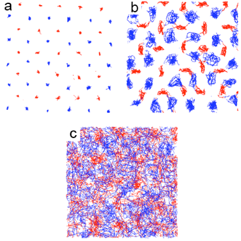
Once we have located the hyperbolic and elliptic points at each instant in time, we can feed their positions into the same tracking algorithms we use to construct the tracer-particle trajectories, and thereby study their dynamics. At low $\mathrm{Re}$, where the underlying flow is a vortex array locked to the magnetic forcing, the hyperbolic and elliptic points lie on a square lattice, as shown in Fig. 2, with the elliptic points in the vortex centers and the hyperbolic points at the vortex corners. As $\mathrm{Re}$ is increased, the special points wander progressively farther from their lattice sites. We observe that the elliptic points move in quasi-circular orbits, while the hyperbolic points move primarily along their stable manifolds. Finally, when $\mathrm{Re}$ is high enough, the special points break free from the lattice and wander freely; in a sense, the lattice melts. We note that the dynamics of the hyperbolic and elliptic points are representative of the dynamics of the flow pattern, rather than of the tracer particles themselves; the individual tracer particles may wander between the vortex cells even in the regime where the special points remain pinned.

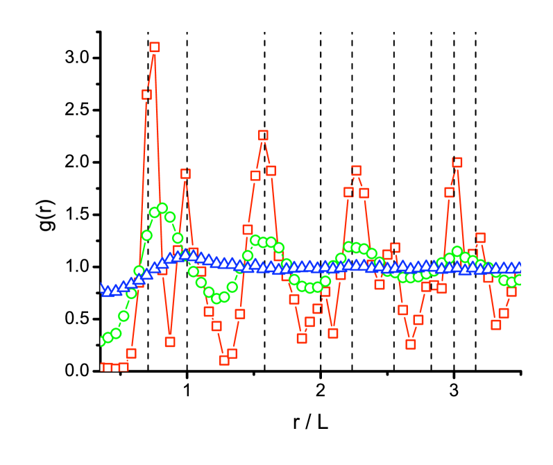
To elucidate the transition between the ordered and disordered states of the topologically special points, we show in Fig. 3 the radial distribution function $g(r)$ g_o of the special point positions for three Reynolds numbers. $g(r)$ is defined to be the mean number density a distance $r$ from a fixed position, normalized by the bulk number density. In an ordered state, $g(r)$ is expected to show a series of peaks corresponding to lattice sites; in a disordered state, however, $g(r)$ should be unity. At $\mathrm{Re}=32$, when the special points are tightly bound to their lattice sites, $g(r)$ is found to be peaked at many of the locations expected for a 2D square lattice. As $\mathrm{Re}$ increases, the peaks broaden and $g(r)$ gradually loses structure. By $\mathrm{Re}=245$, where the special points move freely and the spatial order has vanished, $g(r)$ is unity and the special points form a liquid-like state. To quantify the loss of order, we plot the maximum value of $g(r)$ (corresponding to the height of its first peak) as a function of $\mathrm{Re}$ in Fig. 4.

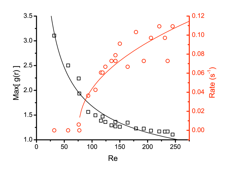
Once the topologically special points can move appreciably around their lattice sites, they undergo pairwise interactions that change the topology of the flow. They can be annihilated in vortex mergers, and new hyperbolic-elliptic pairs are created when vortices split. By recording the number of such events from our special point trajectories, we can measure the rates for each of these processes. The annihilation rate is shown as a function of $\mathrm{Re}$ in Fig. 4; we find that the creation and annihilation rates are equal to within experimental accuracy. As expected, these rates grow substantially as the driving increases. Surprisingly, however, these rates have a clear onset at a critical Re, unlike the gradual decline of $g(r)$. We have also measured other indicators of disorder, including the average of the local speed $\langle\partial u/\partial t\rangle$ and the mean of the largest Lyapunov exponent $\langle\lambda\rangle$. As with $g(r)$, however, these measurements show a continuous change rather than a sharp onset. The lack of a clear threshold in these measurements may be attributed to the averaging of $g(r)$, $\langle\partial u/\partial t\rangle$, and $\langle\lambda\rangle$ over space, time, or both. In contrast, the creation and annihilation of hyperbolic and elliptic point pairs are local in both space and time.

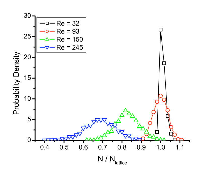
The number of special points in the measurement volume changes in tandem with the rise of the pair creation and annihilation rates. In Fig. 5, we show the PDFs of the number of special points at each instant in time for several Reynolds numbers. As $\mathrm{Re}$ increases, the pattern coarsens and the mean number drops, consistent with the well-known inverse energy cascade in 2D turbulence Kraichnan (1967). At the same time, the width of the distribution grows, which signals the increased activity of the special points and the corresponding increase in the frequency of topological changes.

In summary, we have developed a method to locate the moving hyperbolic and elliptic points experimentally by measuring the curvature of particle trajectories, and have used them to characterize the dynamics of a 2D flow. As Re is increased, these points gradually unbind from their preferred locations (determined by the forcing), deforming the entire flow pattern. When they are created or annihilated in pairs, starting at $Re\sim 75$, they change the topology of the pattern. The behavior of these points shows that the transition to STC involves two successive stages: a gradual loss of spatial and temporal order followed by a surprising abrupt onset of topological changes. We suggest that new theories of STC may be developed using these topological ideas.