Cyclic sieving on permutations - an analysis of maps and statistics in the FindStat database

Ashleigh Adams¹ North Dakota State University. ashleigh.adams@ndsu.edu , Jennifer Elder² Missouri Western State University. jelder8@missouriwestern.edu , Nadia Lafrenière³ Concordia University. nadia.lafreniere@concordia.ca , Erin McNicholas⁴ Willamette University. emcnicho@willamette.edu , Jessica Striker⁵ North Dakota State University. jessica.striker@ndsu.edu and Amanda Welch⁶ Eastern Illinois University. arwelch@eiu.edu

Abstract.

We perform a systematic study of permutation statistics and bijective maps on permutations using SageMath to search the FindStat combinatorial statistics database to identify apparent instances of the cyclic sieving phenomenon (CSP). Cyclic sieving occurs on a set of objects, a statistic, and a map of order $n$ when the evaluation of the statistic generating function at the $d$ th power of the primitive $n$ th root of unity equals the number of fixed points under the $d$ th power of the map. Of the apparent instances found in our experiment, we prove 34 new instances of the CSP, and conjecture three more. Furthermore, we prove the equidistribution of some statistics and show that some maps have the same orbit structure, thus cyclic sieving holds for more even more pairs of a map and a statistic. The maps which exhibit the CSP include reverse/complement, rotation, Lehmer code rotation, toric promotion, and conjugation by the long cycle, as well as a map constructed by Corteel to swap the number of nestings and crossings, the invert Laguerre heap map, and a map of Alexandersson and Kebede designed to preserve right-to-left minima. Our results show that, contrary to common expectations, actions that exhibit homomesy are not necessarily the best candidates for the CSP, and vice versa.

1. Introduction

In this paper, we continue the study of dynamical phenomena on permutations begun in [12] by searching the FindStat database [28] for apparent instances of the cyclic sieving phenomenon. The cyclic sieving phenomenon (CSP), defined by Reiner, Stanton, and White in 2004 [25], occurs for a set when evaluating a polynomial at particular roots of unity counts elements fixed under corresponding powers of an action. It has been observed on various objects, including tableaux, words, set partitions, paths, permutations, and Catalan objects (see [1, 26, 31]). One challenge to finding instances of this phenomenon is that it is necessary to compute two distinct quantities and show they coincide: orbit structure of an action and root of unity evaluations of a polynomial. Sometimes the action relates to the polynomial evaluation, but not always, so the choice of action and polynomial often requires inspired guessing or representation theoretic motivation. Our approach is the first systematic search for instances of this phenomenon.

The first example in the original CSP paper [25, Theorem 1.1] includes Mahonian permutation statistics under rotation as a special case. Another instance, proved in [4] and also mentioned in [1], is related to the Robinson-Schensted-Knuth correspondence and involves the action that cyclically rotates both rows and columns of a permutation matrix and uses the generating function for the sum of the squares of the $q$ -hook length formula.

The only other occurrences of the cyclic sieving phenomenon on permutations we could find in the literature concerns the map of conjugating by the long cycle $(1,2,\ldots,n)$ . Using representation theory, Barcelo, Reiner, and Stanton proved that some pairs of Mahonian statistics exhibit the bicyclic sieving phenomenon [4, Theorem 1.4], which implies linear combinations of these statistics exhibit the CSP. Later, Sagan, Shareshian and Wachs proved the CSP for statistic-generating functions that correspond to an evaluation of the coefficients of Eulerian polynomials [29]. We discuss these results in Section 8 and show that more statistics have these generating functions and thus exhibit the CSP with respect to the conjugation by the long cycle map.

We describe our main results in the next few paragraphs. Note that when stating CSP results, one typically lists a triple consisting of the set, the polynomial, and the map. For every result in this paper, the set considered is the set of permutations of $[n]$ and the polynomial is the generating function of a permutation statistic. Thus, instead of referring to such a triple, we say a given permutation statistic exhibits the CSP with respect to a given map.

For the first part of the paper, we focus on specific statistics with well-known generating functions and prove the CSP for multiple maps at once. Using existing results on roots of unity and their minimal polynomials, we establish the cyclic sieving phenomenon for maps whose orbits all have the same size $d$ , where $1\leq d\leq n$ (Theorem 4.3). We also consider maps whose orbits all have the same size, which can be larger than $n$ . This is where we introduce the rank of a permutation, which is given by its lexicographical order. We establish that the CSP occurs for the rank with respect to any map whose orbits are all of size $d$ , where $d$ divides $n!$ (Theorem 4.8). Such maps include rotation, Lehmer code rotation and toric promotion. We also find that the $i$ -th entry of a permutation exhibits the CSP with respect to the rotation map (Theorem 4.11), and that toric promotion has the CSP for the number of inversions of the second entry (Corollary 4.13) and a descent variant minus the inversion number (Theorem 4.15).

In the rest of the paper, we focus on maps with certain orbit structures and prove results for multiple statistics paired with those maps. FindStat contains two involutions with no fixed points on permutations: the reverse and complement maps. This orbit structure allows us to prove the CSP by showing that the statistic-generating function satisfies $f(-1)=0$ . In addition to the results related to Mahonian statistics, this form of the problem allows us to utilize two main techniques: (1) finding the specific form of the statistic generating function, and using those properties to show that $f(-1)=0$ (for example, Theorem 5.3), and (2) by constructing specific involutions $\psi:S_{n}\rightarrow S_{n}$ to pair the permutations such that $\text{stat}(\sigma)$ and $\text{stat}(\psi(\sigma))$ have the opposite parity (for example, Theorem 5.37). Using these two methods, we show that both maps exhibit CSP for many statistics, including the number of circled entries of the shifted recording tableau (Theorem 5.7 ), the prefix exchange distance (Theorem 5.30), and the number of visible inversions (Theorem 5.35).

FindStat also contains two involutions on $S_{n}$ that we show in Lemmas 6.4 and 6.5 have $2^{n-1}$ fixed points: the Corteel and the invert Laguerre heap maps. The Corteel map switches properties of a permutation known as crossings and nestings, while the invert Laguerre heap map can be seen as a reflection of an arc diagram created using points in the plane of the form $(i,\sigma(i))$ . As with the reverse and complement, proving the CSP reduces to showing that the statistic generating function satisfies $f(-1)=2^{n-1}$ . The proof techniques in this section are more complex; in particular, they involve some proofs of statistic equidistribution that may be of independent interest (Lemmas 6.11 and 6.13). Using this approach, we prove that in addition to the number of nestings and crossings, a number of statistics exhibit the CSP under the Corteel and invert Laguerre heap maps. These include the cycle descent number (Theorem 6.12) and several permutation pattern statistics, such as the number of occurrences of the pattern $13-2$ and the pattern $12-3$ (Theorems 6.7 and 6.16 respectively).

The Alexandersson-Kebede map is an involution on permutations that preserves right-to-left minima, introduced in [2] in order to give a bijective proof of an identity regarding derangements. This map has $2^{\lfloor\frac{n}{2}\rfloor}$ fixed points, and we show that it exhibits the CSP for statistics related to extrema of partial permutations and to inversions (Theorems 7.4 and 7.10 and Corollary 7.7).

While we focused our study on the maps found in FindStat, it is important to note that if two bijections share the same orbit structure and one exhibits the CSP under a statistic, then the other does as well. Thus, our results generalize beyond the maps found in FindStat.

Remark 1.1.

In [12], we conducted a similar study of a dynamical phenomenon on permutations called homomesy, using the FindStat database. In past studies, some objects and actions were found that exhibit both homomesy and the CSP; it was therefore often believed that the best candidates for exhibiting the CSP were known occurrences of homomesy, and vice versa. The results of the two projects combined allow us to conclude that even though several pairs exhibit both phenomena (such as the complement with nine of the statistics found in this paper; see Remark 3.1), many actions are prone to only the CSP (such as the Corteel map; see Section 6), or are excellent candidates for homomesy while exhibiting very few CSPs (such as the Lehmer code rotation; see [12, Section 4]).

The paper is structured as follows. In Section 2, we give definitions related to permutations and the CSP. In Section 3 we discuss our systematic approach to the CSP using FindStat. In Section 4, we give our first examples of CSPs on familiar statistics and maps, whose proofs are relatively simple. We organize the rest of the paper by maps, beginning with reverse and complement (Section 5), followed by the Corteel and invert Laguerre heap maps (Section 6), the Alexandersson-Kebede map (Section 7), and finally, conjugation by the long cycle (Section 8). Sections 5 and 6 each end with conjectures.

Acknowledgments

We thank Theo Douvropoulos for suggesting to extend the methods of our previous paper [12] to the cyclic sieving phenomenon and the developers of SageMath and FindStat for developing computational tools used in this research. This research began during the authors’ Jan. 2023 visit to the Institute for Computational and Experimental Research in Mathematics in the Collaborate@ICERM program. Much of it was completed at the 2023 Dynamical Algebraic Combinatorics mini-conference at North Dakota State University, with funding from NSF grant DMS-2247089 and the NDSU foundation. JS acknowledges support from Simons Foundation gift MP-TSM-00002802 and NSF grant DMS-2247089.

2. Background

In this section, we collect background information on permutations (Subsection 2.1) and the CSP (Subsection 2.2). Readers familiar with these notions may skip the corresponding subsections or refer to them as needed.

2.1. Permutations

Definition 2.1.

A permutation of $[n]:=\{1,2,\ldots n\}$ is a bijective map $\sigma:[n]\rightarrow[n]$ . We often denote a permutation $\sigma$ as an ordered list $\sigma_{1}\sigma_{2}\ldots\sigma_{n}$ where $\sigma_{i}=\sigma(i)$ , and refer to this as the one-line notation of $\sigma$ . The set of permutations of $[n]$ is often denoted as $S_{n}$ .

We define below a few common maps and statistics on the set of all permutations; less familiar maps and statistics will be defined in the relevant sections.

Definition 2.2.

For a permutation $\sigma=\sigma_{1}\ldots\sigma_{n}$ , the reverse of $\sigma$ is $\mathcal{R}(\sigma)=\sigma_{n}\ldots\sigma_{1}$ , and the complement of $\sigma$ is $\mathcal{C}(\sigma)=(n+1-\sigma_{1})\ldots(n+1-\sigma_{n})$ . That is, $\mathcal{R}(\sigma)_{i}=\sigma_{n+1-i}$ and $\mathcal{C}(\sigma)_{i}=n+1-\sigma_{i}$ . Furthermore, the inverse of $\sigma$ , denoted $\mathcal{I}(\sigma),$ is the permutation such that $\mathcal{I}(\sigma)\circ\sigma=\sigma\circ\mathcal{I}(\sigma)=1\cdots n$ , and the rotation of $\sigma$ is $\textnormal{Rot}(\sigma)=\sigma_{2}\sigma_{3}\ldots\sigma_{n}\sigma_{1}$ .

Definition 2.3.

We say that $(i,j)$ is an inversion of a permutation $\sigma=\sigma_{1}\sigma_{2}\ldots\sigma_{n}$ if $i<j$ and $\sigma_{j}<\sigma_{i}$ . We write $\textnormal{Inv}(\sigma)$ for the set of inversions in $\sigma$ . We say that $(\sigma_{i},\sigma_{j})$ is an inversion pair of $\sigma$ if $(i,j)$ is an inversion of $\sigma$ . The inversion number of a permutation $\sigma$ , denoted $\textnormal{inv}(\sigma)$ , is the number of inversions.

We say that $i$ is a descent whenever $\sigma_{i}>\sigma_{i+1}$ . We write $\textnormal{Des}(\sigma)$ for the set of descents in $\sigma$ , and $\textnormal{des}(\sigma)$ for the number of descents. If $i\in[n-1]$ is not a descent, we say that it is an ascent. The major index of $\sigma$ , denoted $\textnormal{maj}(\sigma)$ , is the sum of its descents.

We say that $\sigma_{i}$ is a left-to-right-maximum of $\sigma$ if there does not exist $j<i$ such that $\sigma_{j}>\sigma_{i}$ . Left-to-right minima, right-to-left maxima, and right-to-left minima are defined similarly.

Definition 2.4.

Let $\sigma=\sigma_{1}\ldots\sigma_{n}$ be a permutation. We define the first fundamental transform, denoted $\mathcal{F}(\sigma)$ , as follows:

•

Place parenthesis $($ to the left of $\sigma_{1}$ , and $)$ to the right of $\sigma_{n}$ .
•

Before each left-to-right maximum in $\sigma$ , insert a parenthesis pair $)($ .

The resulting parenthesization is the cycle decomposition for $\mathcal{F}(\sigma)$ [28]. For example, for $\sigma=241365$ , we have $\mathcal{F}(\sigma)=(2)(413)(65)$ .

Remark 2.5.

We note that Stanley defines the inverse of $\mathcal{F}$ as the fundamental bijection [35, Page 23], which is also known as the first fundamental transform. Stanley shows that each cycle in $\sigma$ is mapped to a left-to-right maximum in $\mathcal{F}^{-1}(\sigma)$ . Thus $\mathcal{F}$ also maps each left-to-right maximum to a cycle in $\mathcal{F}(\sigma)$ . For clarity within the context of this paper, we use the definition given on FindStat, even though it uses a convention opposite to that of Stanley.

We also study statistics related to permutation patterns of length $3$ .

Definition 2.6.

Let $\pi=abc\in S_{3}$ and $\sigma\in S_{n}$ . The permutation $\sigma$ contains the pattern $abc$ if there exist $1\leq i<j<k\leq n$ such that $\sigma_{i},\sigma_{j},\sigma_{k}$ are in the same relative order as $a,b,c$ . The permutation $\sigma$ contains the consecutive pattern $a-bc$ if, in addition, $k=j+1$ , that is, if $\sigma_{j}$ and $\sigma_{k}$ are consecutive in the one-line notation of $\sigma$ .

Finally, we define and give an example of a statistic generating function, as these are central objects in this paper.

Definition 2.7.

Let $n\geq 2$ be an integer, and $\textrm{stat}(\sigma)$ be a permutation statistic defined on all $\sigma\in S_{n}$ . A statistic generating function on $S_{n}$ is a polynomial defined as follows:

f(q)=\sum_{\sigma\in S_{n}}q^{\textrm{stat}(\sigma)}.

Note that one immediate consequence of this definition is that $f(1)=n!$ .

Example 2.8.

We note that in $S_{3}$ , there is one permutation with 0 descents, four permutations with 1 descent, and one permutation with 2 descents. Therefore,

f(q)=\sum_{\sigma\in S_{3}}q^{\textrm{des}(\sigma)}=1+4q^{1}+q^{2}.

We say that two statistics are equidistributed if they have the same statistic generating function.

2.2. The cyclic sieving phenomenon

In 2004, the notion of cyclic sieving was first introduced by Reiner, Stanton, and White with the following definition.

Definition 2.9 ([25]).

Given a set $S$ , a polynomial $f(q)$ , and a bijective action $g$ of order $n$ , the triple $(S,f(q),g)$ exhibits the cyclic sieving phenomenon if, for all $d$ , $f(\zeta^{d})$ counts the elements of $S$ fixed under $g^{d}$ , where $\zeta=e^{2\pi i/n}$ .

While at first glance it seems unlikely to find such a triple that both works and is of interest, there have been many examples. In [31], Sagan surveyed the current literature to show examples of CSP involving mathematical objects such as Coxeter groups, Young tableaux, and the Catalan numbers. Further, more examples of CSP on mathematical objects such as words, paths, matchings and crossings can be found at the online Symmetric Functions Catalog [1] maintained by Alexandersson. For a brief and insightful introduction to cyclic sieving, we refer readers to [26], where more examples of CSP occurring for a variety of mathematical objects can be found.

In a paper pre-dating the original definition of CSP [38], Stembridge presented the “ $q=-1$ ” phenomenon that coincides with the CSP when the order of the bijective action is $2$ . In that case, showing that the triple exhibits CSP is equivalent to showing that $f(1)$ equals the cardinality of $S$ and $f(-1)$ is the number of fixed points of the bijection. So, if the action $g$ is an involution, then $f(-1)$ gives a closed form enumeration of the fixed points. And thus $f(1)-f(-1)$ counts the number of elements in orbits of size $2$ . This “ $q=-1$ ” phenomenon helped inspire the definition of the CSP and is integral to the work of this paper, as many of the maps we investigate are involutions.

3. A systematic, statistic-oriented approach to the CSP

Our approach to finding instances of the CSP is as follows: rather than test pairs of specific maps and polynomials that arise in other research, we search for cyclic sieving systematically. For this study, we focused our attention on maps and statistics on permutations in FindStat—an online database of combinatorial statistics developed by Berg and Stump in 2011 [28]. Like other fingerprint databases highlighted in [6], FindStat is a searchable collection of information about a class of mathematical objects. The interface between SageMath [36] and FindStat makes it possible to not only retrieve stored information from the FindStat database, but use that information to discover new connections.

For each statistic on permutations, we used SageMath to evaluate the statistic generating function at the appropriate roots of unity to test whether this matched the corresponding fixed point counts of any bijective map on permutations in the database. The experiment we conducted was based on the FindStat database as of January 30, 2024, and was done for all permutations of $n=4$ to $6$ elements. This range in $n$ was chosen to limit false negatives, as some statistics are not meaningful for very small permutations, and to be executed in a reasonable amount of time. We looked at all pairs made of the 24 bijective maps and 400 permutation statistics in FindStat, and we found counter-examples to the cyclic sieving phenomenon for all but 202 pairs. After removing repetitions for pairs that have the same orbit structure and the same statistic generating function, we found 37 apparent instances of the CSP, meaning distinct pairs made of an orbit structure and a polynomial. Four of these were the previously proven CSPs discussed in the introduction. Of the remaining 33, we prove 30 new instances of the CSP, prove one for only odd values of $n$ and conjecture it is true for even $n$ , and leave two others as conjectures. We also provide three new interesting proofs of equidistribution of statistics. In total, the number of pairs of a map and a permutation statistic from FindStat for which we have a proof of cyclic sieving for all values of $n\geq 4$ is $196$ .

For all other pairs of a permutation statistic and a map in FindStat, we found counter-examples to the CSP. This means that pairs of maps and statistics in FindStat that are not mentioned here do not exhibit the CSP, or at least not for all values of $n\geq 4$ . While working on the project, we noticed that it is possible that some statistics exhibit the CSP only for an infinite subset of values of $n$ . We give here three examples of statistics that have the CSP for only all odd or all even values of $n$ (see Theorem 5.12). We did not attempt a systematic study of the CSP for only odd or even values. Including these results, we prove 33 instances of the CSP in total.

In the statements about our results, we refer to statistics and maps by their name as well as their FindStat identifier (ID). This makes it easier for the reader to find the associated FindStat webpage. For example, the URL for Statistic $356$ , the number of occurrences of the pattern $13-2$ , is: http://www.findstat.org/StatisticsDatabase/St000356. The highest ID for a bijective map on permutations was 310, and the highest ID for a statistic on permutations was 1928.

Due to the breath of the FindStat database, our study gives a good portrait of occurrences of the phenomenon on permutations. Our study also gives us a good portrait of the differences between homomesy and the CSP for permutation maps and statistics.

Remark 3.1.

As noted in Remark 1.1, past studies found several examples of sets and actions that exhibit both homomesy and the CSP (see e.g. [22, p.2]). It is therefore interesting to consider how many of the map–statistic pairs from our homomesy paper [12], as well as the follow-up [11], also exhibit the CSP. We found the only pairs of maps and statistics that exhibit both homomesy and the CSP are in Sections 4 and 5 of this paper. We list these below, organized by map.

•

Lehmer code rotation: Statistic 20.
•

Rotation: Statistics 54, 740, 1806, and 1807.
•

Both reverse and complement: Statistic 18 (Mahonian); Statistics 495, 538, and 677; Statistics 21 and 1520 (for $n$ even); and Statistics 836 and 494 (for $n$ odd).
•

Complement but not reverse: Statistics 4, 20, and 692 (Mahonian); Statistics 1114 and 1115.
•

Reverse but not complement: Statistics 304, 305, 446, and 798 (Mahonian); Statistics 495, 538, and 677.

In this paper, the reverse and complement are paired together as they have the same orbit structure. However, their lists are different in [12] because homomesy does not solely rely on orbit structure. In [11], rotation exhibits homomesy when paired with 34 statistics, but the only statistics that also exhibit the CSP are those related to specific entries. We also note that the Lehmer code rotation exhibits homomesy when paired with 45 statistics, and only exhibits the CSP when paired with one statistic.

In [12], we found nine permutation maps that exhibit homomesy, and six of those maps do not exhibit any instances of the CSP. Similarly, in this paper we consider Corteel and invert Laguerre heap, Alexandersson-Kebede, and conjugation by the long cycle, none of which exhibit any homomesy. Finally, we include the map toric promotion in Section 4 of this paper, but it is an open question whether the map exhibits homomesy for any permutation statistics. We did not investigate the latter, since the toric promotion map was not in FindStat at the time of the investigation.

4. Mahonian statistics, rank, and specific entries

In this section, we prove some initial CSPs involving well-known statistics with maps whose orbits all have the same size.

4.1. Mahonian statistics

Our first proofs of the cyclic sieving phenomenon concern a large family of statistics; many of these are among the most well-known permutation statistics.

Definition 4.1.

A Mahonian statistic Stat is a statistic on permutations whose generating function is

\sum_{\sigma\in S_{n}}q^{\textnormal{Stat}(\sigma)}=(1+q)(1+q+q^{2})\ldots(1+q+\ldots+q^{n-1})=:[n]_{q}!.

Here, $[n]_{q}!=[1]_{q}[2]_{q}\cdots[n]_{q}$ where for any $k\in\mathbb{N}$ , $[k]_{q}$ denotes the $q$ -analogue $[k]_{q}:=1+q+\ldots+q^{k-1}$ .

As of January 30, 2024, FindStat contained 19 Mahonian statistics. Before studying cyclic sieving of these statistics, we gather in the following proposition references showing that these statistics are indeed Mahonian. See Definition 2.3 for the definitions of Statistics 4, 18, and 305. For brevity, we do not include the definitions of the rest of these statistics, as the interested reader can easily find the definitions in the given references and on FindStat.org.

Proposition 4.2.

The following statistics on permutations are Mahonian:

•

Statistic $4$ : The major index
•

Statistic $18$ : The number of inversions
•

Statistic $156$ : The Denert index
•

Statistic $224$ : The sorting index
•

Statistic $246$ : The number of non-inversions
•

Statistic $304$ : The load
•

Statistic $305$ : The inverse major index
•

Statistic $334$ : The maz index, the major index after replacing fixed points by zeros
•

Statistic $339$ : The maf index
•

Statistic $446$ : The disorder
•

Statistic $692$ : Babson and Steingrímsson’s statistic stat
•

Statistic $794$ : The mak
•

Statistic $795$ : The mad
•

Statistic $796$ : The stat^′
•

Statistic $797$ : The stat^′′
•

Statistic $798$ : The makl
•

Statistic $833$ : The comajor index
•

Statistic $868$ : The aid statistic in the sense of Shareshian-Wachs
•

Statistic $1671$ : Haglund’s hag

Proof.

All these statistics are known in the literature to be Mahonian or can be seen to be easily equidistributed with Mahonian statistics. The original investigation of the inversion number statistic was done by Olinde Rodrigues, who found a generating function [27]. Later, Percy MacMahon found the statistic-generating function for what was called the greater index, and is now called the major index [20]. A more detailed story appears in [35, p. 98], and proofs of the major index and number of inversions being Mahonian are reproduced, for example, in [35] as Proposition 1.4.6 and Corollary 1.3.13, respectively.

We now discuss the rest of the statistics in roughly the order given above.

The Denert index is shown to be Mahonian in [15, §2]. The sorting index was introduced in [21], and shown there to be Mahonian.

The number of non-inversions is equidistributed with the number of inversions through the complement map that sends an inversion $(i,j)$ to a non-inversion, and vice versa. Therefore, the number of non-inversions is also Mahonian. Similarly, the inverse major index is the major index of the inverse, and therefore is equidistributed with the major index through the inverse map. The load is defined on permutations as the major index of the reverse of the inverse, and, as such, is Mahonian. Also, the comajor index is obtained from the major index by applying both the reverse and the complement, and is therefore equidistributed with the major index.

We claim that the disorder of a permutation is the comajor index of the inverse, meaning that it is also Mahonian. To show it, we use the information in [12, proof of Proposition 5.51] that the disorder of $\sigma$ is given by $\sum_{i=1}^{n-1}(n-1)\delta_{(\text{$i+1$ appears to the left of $i$ in $\sigma$})}$ . Hence, this is equivalent to $\sum_{i=1}^{n-1}(n-1)\delta_{(\text{$i$ is a descent of $\sigma^{-1}$})}$ , which is the definition of the comajor index of $\sigma^{-1}$ .

The maz and maf statistics were introduced in [14], where they were shown to be equidistributed with the major index and the number of inversions, so they are Mahonian.

Statistics stat, mak, mad, stat^′, stat^′′, makl, and hag all appear in the work of Babson and Steingrimsson on the translation of Mahonian statistics into permutation patterns, where they are shown to be Mahonian [3].

The aid statistic appear in the work of Shareshian and Wachs, where it is shown to be equidistributed with the major index [33, Theorem 4.1]. ∎

Note the triangle of values of Mahonian statistics appears as sequence A008302 of the Online Encyclopedia of Integer Sequences [16].

The inversion number statistic under rotation is one of the original instances of the CSP proved in [25, Theorem 1.1]. We give a computational proof below that works for any map whose orbits all have the same size $d$ with $1\leq d\leq n$ .

Theorem 4.3.

The Mahonian statistics exhibit the cyclic sieving phenomenon under any map whose orbits all have size $d$ , where $1\leq d\leq n$ .

Proof.

The generating function for any Mahonian statistic is given as

f(q)=[n]_{q}!=\prod_{i=1}^{n}[i]_{q}=\prod_{i=1}^{n}(q^{i-1}+q^{i-2}+\ldots+1).

Let $g$ be an action whose orbits all have size $d$ with $1\leq d\leq n$ . We consider the primitive $d$ th root of unity, $\zeta=e^{\frac{2\pi\cdot i}{d}}$ . We note that $f(\zeta^{d})=f(1)=n!$ . To prove that $g$ exhibits the CSP with respect to this polynomial, we wish to show $f(\zeta^{k})=0$ for all $1\leq k<d$ .

By definition, $(\zeta^{k})^{d-1}+(\zeta^{k})^{d-2}+\cdots+(\zeta^{k})^{1}+1=0$ for all $k$ values. Thus, we have

	$\displaystyle f(\zeta^{k})$	$\displaystyle=\left(\prod_{i=1}^{d-1}[i]_{\zeta^{k}}\right)\cdot[d]_{\zeta^{k}}\cdot\left(\prod_{i=d+1}^{n}[i]_{\zeta^{k}}\right)$
		$\displaystyle=\left(\prod_{i=1}^{d-1}[i]_{\zeta^{k}}\right)\cdot 0\cdot\left(\prod_{i=d+1}^{n}[i]_{\zeta^{k}}\right)$
		$\displaystyle=0$

as desired. ∎

Defant defines toric promotion as a bijection on the labelings of a graph. In [10], he shows that the order of toric promotion has a simple expression if the graph is a forest. Toric promotion can be applied to the permutation $\sigma$ by considering the path labeled from left to right by $\sigma_{1}\ldots\sigma_{n}$ as graph, then applying toric promotion to that graph. Applying toric promotion to that path graph is equivalent to the following definition directly on permutations:

Definition 4.4.

Let $\sigma$ be a permutation of $[n]$ . Define $\tau_{i,j}(\sigma)=(i,j)\circ\sigma$ if $|\sigma^{-1}(i)-\sigma^{-1}(j)|>1$ , and $\tau_{i,j}(\sigma)=\sigma$ otherwise. Toric promotion (Map 310) is equivalent to multiplying the permutation $\sigma$ by the product $\tau_{n,1}\tau_{n-1,n}\ldots\tau_{1,2}$ .

Using [10, Theorem 1.3], toric promotion on any tree with $n$ vertices has order $n-1$ , and all orbits of toric promotion have size $n-1$ . Consequently, toric promotion divides the set of permutations of $[n]$ into orbits all of size $n-1$ .

Corollary 4.5.

The Mahonian statistics exhibit the cyclic sieving phenomenon under the reverse, complement, toric promotion, and rotation maps.

Proof.

The reverse and complement maps have orbits all of size $2$ . Following the discussion above, the toric promotion has all orbits of size $n-1$ on permutations. The rotation map has orbits all of size $n$ . Thus, we have the result by Theorem 4.3. ∎

Mahonian statistics again appear in Section 8, where we discuss cyclic sieving of linear combinations of these statistics with respect to conjugation by the long cycle.

4.2. Rank

In this subsection, we prove CSPs involving the rank statistic and several maps: reverse, complement, rotation, and Lehmer code rotation.

Definition 4.6.

The rank (Statistic 20) of a permutation of $[n]$ is its position among the $n!$ permutations, ordered lexicographically. This is an integer between $1$ and $n!$ .

Definition 4.7.

The Lehmer code of a permutation $\sigma\in S_{n}$ is $L(\sigma)=(L(\sigma)_{1},\ldots,L(\sigma)_{n})\quad{\text{where}}\quad L(\sigma)_{i}=\#\{j>i\mid\sigma_{j}<\sigma_{i}\}$ . The Lehmer code rotation (Map 149) is a map that sends $\sigma$ to the unique permutation $\tau\in S_{n}$ such that every entry in the Lehmer code of $\tau$ is cyclically (modulo $n+1-i$ ) one larger than the Lehmer code of $\sigma$ .

Theorem 4.8.

The rank of a permutation exhibits the cyclic sieving phenomenon under any action whose orbits all have size $d$ , where $d$ divides $n!$ .

Proof.

Every permutation is given a unique rank from 1 to $n!$ . So the generating function of the rank statistic is

f(q)=\sum_{j=1}^{n!}q^{j}.

Suppose $g$ is an action whose orbits all have size $d|n!$ . We note that $f(1)=n!$ . We consider the roots of unity $\zeta^{k}=e^{\frac{2\pi\cdot i}{d}k}$ for $1\leq k<d$ . Because $d$ divides $n!$ , we have

$\displaystyle f(\zeta^{k})$	$\displaystyle=$	$\displaystyle\sum_{j=1}^{n!}\zeta^{kj}$
	$\displaystyle=$	$\displaystyle\frac{n!}{d}\sum_{j=1}^{d}e^{\frac{2\pi\cdot i}{d}j}$
	$\displaystyle=$	$\displaystyle 0$

as desired. ∎

Corollary 4.9.

The rank (Statistic $20$ ) exhibits the cyclic sieving phenomenon under the actions of the reverse, complement, toric promotion, rotation, and Lehmer code rotation maps.

Proof.

The reverse and complement maps have orbits all of size $2$ . The rotation map has orbits all of size $n$ . By [12, Theorem 4.8], Lehmer code rotation has orbits all of size $\operatorname{lcm}(1,2,\ldots,n)$ , which divides $n!$ . The result follows by Theorem 4.8 above. ∎

Remark 4.10.

It is interesting that this is the only statistic from FindStat for which the Lehmer code rotation exhibits the CSP, while we showed in [12] that this map exhibits many homomesies with statistics in FindStat. The study of both phenomena on Lehmer code rotation allows us to counter the notion that homomesy and cyclic sieving occur for the same actions (see Remark 1.1).

4.3. Specific entries and rotation

In the prior two subsections, we showed the rotation map exhibits the CSP for Mahonian statistics and the rank of a permutation. Here we prove an additional CSP for the rotation map, which includes the following FindStat statistics:

•

Statistic 54: The first entry of a permutation,
•

Statistic 740: The last entry of a permutation,
•

Statistic 1806: The upper middle entry of a permutation,
•

Statistic 1807: The lower middle entry of a permutation.

In fact, any specific entry statistic exhibits the CSP with respect to rotation.

Theorem 4.11.

The $i$ -th entry of a permutation exhibits the cyclic sieving phenomenon occurs under the rotation map.

Proof.

The generating function for the $i$ -th entry of a permutation is $f(q)=\sum_{j=1}^{n}(n-1)!q^{j}$ , for all $1\leq i\leq n$ .

Recall the orbits of rotation of permutations of $n$ are all of cardinality $n$ , so to exhibit the CSP with polynomial $f$ , we need $f(\zeta^{k})=0$ for all $1\leq k<n$ .

Let $1\leq k\leq n-1$ , and $\zeta=e^{\frac{2\pi i}{n}}$ . Then

f(\zeta^{k})=\sum_{j=1}^{n}(n-1)!\zeta^{jk}=(n-1)!\underbrace{\sum_{j=1}^{n}\zeta^{jk}}_{0}=0

as desired. ∎

4.4. Inversions of a specific entry and toric promotion

In the prior two subsections, we showed the toric promotion map exhibits the CSP for Mahonian statistics and the rank of a permutation. Here we prove two additionals CSP for the toric promotion map.
The number of inversions of the $i$ -th entry of a permutation $\sigma$ is the number of inversions $\{i<j\mid\sigma(j)<\sigma(i)\}$ , where $i$ is fixed. This includes the following FindStat statistics:

•

(Statistic 54) The first entry of a permutation. The number of inversions of the first entry equals Statistic 54 minus one.
•

(Statistic 1557) The number of inversions of the second entry
•

(Statistic 1556) The number of inversions of the third entry

The number of inversions of the $i$ -th entry is a statistic that has the CSP for some maps whose orbits all have the same size.

Theorem 4.12.

The number of inversions of the $i$ -th entry exhibits the cyclic sieving phenomenon under any map whose orbits all have size $n+1-i$ .

Proof.

We use the fact that permutations of $[n]$ are in bijection with Lehmer codes, which are sequences of $n$ numbers, such that the $i$ -th takes a value between $0$ and $n-i$ . There are $n!$ possible Lehmer codes, and the Lehmer code $(a_{1},\ldots,a_{n})$ corresponds to the unique permutation that has $a_{i}$ inversions of the $i$ -th entry for each $1\leq i\leq n$ . For more details on this bijection with Lehmer codes, see for example [17, p.12]. Since the number of Lehmer codes with $i$ -th entry equal to $k$ is $\frac{n!}{n-i+1}$ for any value of $k$ between $0$ and $n-i$ , there are exactly $\frac{n!}{n-i+1}$ permtutations with $k$ inversions of the $i$ -th entry, and the statistic generating function is

f(q)=\frac{n!}{n-i+1}\sum_{j=0}^{n-i}q^{j}.

This generating function is $0$ when $q=e^{2\pi ik/(n+1-i)}$ with $k<(n+1-i)$ , and is equal to $n!$ when $k=(n+1-i)$ . Therefore, if all orbits have size $n+1-i$ , $f(e^{2\pi ik/(n+1-i)})=0$ for any $k<n+1-i$ , so a map with all orbits of size $n+1-i$ exhibits the CSP with the number of inversions of the $i$ -th entry. ∎

Note that the above result allows to recover the result of Theorem 4.11 for the first entry, a CSP for the reverse and complement maps with the number of inversions of the $(n-1)$ st entry, and the following corollary about toric promotion (see Definition 4.4).

Corollary 4.13.

The number of inversions of the second entry (Statistic $1557$ ) exhibits the cyclic sieving phenomenon under the toric promotion map.

There is one more statistic that FindStat suggests as exhibiting the CSP for toric promotion.

Definition 4.14.

For $\sigma\in S_{n}$ , define the following descent variant $\partial(\sigma)=\sum_{i\in\textnormal{Des}(\sigma)}{i(n-i)}$ .

Theorem 4.15.

The descent variant $\partial$ minus the number of inversions (Statistic 1911) exhibits the cyclic sieving phenomenon under the toric promotion map.

Proof.

By [39, Remark 1.5], the generating function for Statistic 1911 is

\sum_{\sigma\in S_{n}}q^{\partial(\sigma)-\textnormal{inv}(\sigma)}=n\prod_{i=1}^{n-1}\frac{1-q^{i(n-1)}}{1-q^{i}}.

The factor of this product when $i=1$ is $\displaystyle\frac{1-q^{n-1}}{1-q}=\sum_{i=0}^{n-2}q^{i}$ , which equals $0$ when $q=e^{2\pi ik/(n-1)}$ for $1\leq k<n-1$ . ∎

5. Reverse and complement (Maps 64 and 69)

For $n\geq 2$ , both the reverse and complement maps (Definition 2.2) are involutions with no fixed points. Thus all of their orbits are of size two. To show that a statistic exhibits the cyclic sieving phenomenon under the reverse and complement, we can reduce the problem to showing $f(-1)=0$ , where $f$ is the statistic generating function

f(q)=\sum_{\sigma\in S_{n}}q^{\textrm{stat}(\sigma)}.

We can do so by finding the statistic generating function and evaluating at $-1$ , though often this is a difficult task. Instead, we may show $f(-1)=0$ by showing that the number of permutations that exhibit an odd statistic value equals the number of permutations that exhibit an even statistic value. One way of doing this is to pair the permutations using the reverse or complement; however, we do not need to restrict ourselves to these maps. Any bijection that pairs the permutations into orbits of size 2 where there is a change in parity across the orbit works. Due to this, we can often define the pairing by composing with a specific transposition.

Remark 5.1.

The results in this section are all related to the fact that all of the orbits under the reverse and complement are of size two. These results can be applied to any permutation map that has the same orbit structure. In particular, any transposition has all orbits of size two and thus exhibits the CSP for all statistics examined in this section.

Recall we proved Corollaries 4.5 and 4.9 that the 19 Mahonian statistics and the rank (Statistic 20) exhibit the CSP under the reverse and complement maps. In this section, we prove the following additional statistics exhibit the cyclic sieving phenomenon with respect to these maps.

•

Theorem 5.3 and Corollary 5.4
- –
  
  Statistic 7: The number of saliances (right-to-left maxima)
- –
  
  Statistic 31: The number of cycles in the cycle decomposition
- –
  
  Statistic 314: The number of left-to-right-maxima
- –
  
  Statistic 541: The number of indices greater than or equal to 2 such that all smaller indices appear to its right
- –
  
  Statistic 542: The number of left-to-right-minima
- –
  
  Statistic 991: The number of right-to-left minima
•
Theorem 5.6
- –
  
  Statistic 216: The absolute length
- –
  
  Statistic 316: The number of non-left-to-right-maxima
•

Theorem 5.7 (Statistic 864): The number of circled entries of the shifted recording tableau
•

Theorem 5.9 (Statistic 495): The number of inversions of distance at most 2
•

Theorem 5.13 (Statistic 483): The number of times a permutation switches from increasing to decreasing or decreasing to increasing
•

Theorem 5.15 (Statistic 538): The number of even inversions
•

Theorem 5.18 (Statistic 638): The number of up-down runs
•

Theorem 5.20 (Statistic 677): The standardized bi-alternating inversion number
•

Theorem 5.22 (Statistic 809): The reduced reflection length
•

Theorem 5.25 (Statistic 1579): The number of cyclically simple transpositions needed to sort a permutation
•
Theorem 5.30
- –
  
  Statistic 1076: The minimal length of a factorization of a permutation into transpositions that are cyclic shifts of $(12)$
- –
  
  Statistic 1077: The prefix exchange distance
•
Theorem 5.32
- –
  
  Statistic 1114: The number of odd descents
- –
  
  Statistic 1115: The number of even descents
•

Theorem 5.35 (Statistic 1726): The number of visible inversions
•
Theorem 5.37:
- –
  
  Statistic 423: The number of occurrences of the pattern 123 or of the pattern 132
- –
  
  Statistic 428: The number of occurrences of the pattern 123 or of the pattern 213
- –
  
  Statistic 436: The number of occurrences of the pattern 231 or of the pattern 321
- –
  
  Statistic 437: The number of occurrences of the pattern 312 or of the pattern 321

Additionally, we prove the following.

•
Theorem 5.12
- –
  
  Statistic 21: The number of descents for $n>1$ and $n$ an even number (but not for $n$ odd).
- –
  
  Statistic 836: The number of 2-descents, for $n>2$ and $n$ an odd number (but not for $n$ even)
- –
  
  Statistic 1520: The number of strict 3-descents, for $n>3$ and $n$ an even number (but not for $n$ odd)
•

Theorem 5.10 (Statistic 494): The number of inversions of distance at most 3 when $n$ is odd. We leave as Conjecture 5.38 that this also holds for $n$ even.

We organize our results based on the techniques we used in proving them, be it by using the generating function for the statistic, or bijectively by pairing the permutations to show the number that exhibit an odd statistic equals the number that exhibit an even statistic. However, we note that it may be possible to prove the results using more than one technique.

5.1. Factoring the generating functions

We begin with those results that make use of the generating function.

We prove the following lemma for use in Theorem 5.3.

Lemma 5.2.

The following statistics are equidistributed:

•

Statistic $7$ : The number of saliances (right-to-left maxima),
•

Statistic $31$ : The number of cycles in the cycle decomposition,
•

Statistic $314$ : The number of left-to-right-maxima,
•

Statistic $542$ : The number of left-to-right-minima,
•

Statistic $991$ : The number of right-to-left minima.

Proof.

Under the complement map, the left-to-right maxima are mapped to left-to-right minima, and similarly the right-to-left maxima are mapped to right-to-left minima. Under the reverse map, the left-to-right maxima are mapped to right-to-left maxima. Thus, Statistics 7, 314, 542, and 991 are all equidistributed.

The fundamental bijection (as defined in Remark 2.5) sends the number of cycles to the number of left-to-right maxima [35, Proposition 1.3.1], which completes the result. ∎

Theorem 5.3.

For $n\geq 2$ , the following statistics exhibit the cyclic sieving phenomenon under the reverse and complement maps.

•

Statistic $7$ : The number of saliances (right-to-left maxima),
•

Statistic $31$ : The number of cycles in the cycle decomposition,
•

Statistic $314$ : The number of left-to-right-maxima,
•

Statistic $542$ : The number of left-to-right-minima,
•

Statistic $991$ : The number of right-to-left minima.

Proof.

For $n\geq 2$ , we claim the number of cycles in the cycle decomposition has a generating function that can be defined recursively. That is, the statistic generating function $f(q)$ is of the form

f(q)\coloneqq f_{n}(q)=q\prod_{k=1}^{n-1}(q+k)=(q+(n-1))f_{n-1}(q)=qf_{n-1}(q)+(n-1)f_{n-1}(q).

One can directly verify that $f_{1}(q)=q$ and $f_{2}(q)=q(q+1)$ .

Now consider $S_{n}$ and $f_{n}(q)$ when $n\geq 3$ , and let $\sigma\in S_{n}$ . If $\sigma$ is such that the element $n$ is in a cycle on its own, then $\sigma$ has one more cycle than its restriction to $[n-1]$ ; this is accounted for in the generating function with $qf_{n-1}(q)$ . If $\sigma$ is such that the element $n$ is contained in a cycle with another element, we have $(n-1)$ ways of adding $n$ in front of a number in a cycle in a permutation of $[n-1]$ , accounted for with $(n-1)f_{n-1}(q)$ . Thus the generating function has the recursive and closed forms as seen above.

This closed form for the generating function allows us to see that

\displaystyle f_{n}(-1)

\displaystyle=(-1)(-1+1)\prod_{i=2}^{n-1}(-1+k)=0

as desired.

From Lemma 5.2, the statistics in our theorem statement are all equidistributed, which concludes our proof. ∎

Corollary 5.4.

For $n\geq 2$ , the number of indices greater than or equal to $2$ such that all smaller indices appear to its right (Statistic $541$ ) exhibits the cyclic sieving phenomenon under the reverse and complement maps.

Proof.

We note that for $n\geq 2$ , $q\cdot f(q)=f_{n}(q)$ , where $f_{n}(q)$ is defined in the proof of Theorem 5.3. This is because the number of indices greater than or equal to 2 of a permutation such that all smaller indices appear to its right is exactly the definition of the number of left-to-right minima minus one.

Since $\frac{f_{n}(-1)}{-1}=0$ , then $f(-1)=0$ as desired. ∎

Definition 5.5.

The absolute length of a permutation of $[n]$ is defined as $n$ minus the number of cycles in the cycle decomposition.

Theorem 5.6.

For $n\geq 2$ , the following statistics exhibit the cyclic sieving phenomenon under the reverse and complement maps.

•

Statistic $216$ : The absolute length,
•

Statistic $316$ : The number of non-left-to-right-maxima.

Proof.

Recall from Theorem 5.3 $f_{n}(q)=q\prod_{k=1}^{n-1}(q+k)$ is the generating function for the number of left-to-right-maxima. Thus the generating function for the number of non-left-to-right-maxima is

f(q)=\sum_{\sigma\in S_{n}}q^{n-\mbox{number of left-to-right-maxima}(\sigma)}=q^{n}f_{n}(q^{-1}).

We already showed in Theorem 5.3 that $f_{n}(-1)=0$ . So here we have

f(-1)=(-1)^{n}f_{n}((-1)^{-1})=(-1)^{n}f_{n}(-1)=0.

From Lemma 5.2, we recall that the number of cycles in the cycle decomposition of $\sigma$ is equidistributed with the number of left-to-right minima. Together with Definition 5.5, then the absolute length also has statistic generating function $q^{n}f_{n}(q^{-1})$ . So the result follows. ∎

In the previous results, the generating functions were related to each other, and could easily be proven using elementary techniques. The following theorem relies on work of Sagan [30] and Schur [32] on generating functions related to shifted tableau.

Theorem 5.7.

For $n\geq 2$ , the number of circled entries of the shifted recording tableau (Statistic 864) exhibits the cyclic sieving phenomenon under the reverse and complement maps.

Proof.

A shifted partition shape of $n$ is a list of strictly decreasing numbers summing to $n$ ; the diagram of a shifted partition is drawn with each row indented one more box than the previous. There is a bijection (analogous to the Robinson-Schensted correspondence) between permutations and pairs of shifted standard tableau $(P,Q)$ of the same shape where $Q$ has a subset of its non-diagonal entries circled [30, Theorem 3.1]. Since this is a bijection, all possibilities of circled entries appear. The bijection gives a combinatorial proof of the identity [30, Corollary 3.2] (originally due to Schur [32])

n!=\sum_{\lambda\models n}2^{n-\ell(\lambda)}g_{\lambda}^{2},

where the sum is over all shifted partition shapes $\lambda$ of $n$ , $\ell(\lambda)$ is the number of rows of $\lambda$ (so that $n-\ell(\lambda)$ is the number of non-diagonal entries), and $g_{\lambda}$ is the number of shifted standard tableaux of shape $\lambda$ . The generating function for the number of circled entries is

f_{n}(q)=\sum_{\lambda\models n}(1+q)^{n-\ell(\lambda)}g_{\lambda}^{2},

and we obtain

f_{n}(-1)=\sum_{\lambda\models n}(1-1)^{n-\ell(\lambda)}g_{\lambda}^{2}=0

as desired. ∎

5.2. Bijective Proofs

In this subsection, we consider theorems proved by pairing the permutations so that the statistic changes in parity across the pair. First, we include those we paired with either the reverse or the complement map.

Definition 5.8.

Let $\sigma=\sigma_{1}\sigma_{2}\ldots\sigma_{n}\in S_{n}$ for $n\geq 2$ . An inversion of distance $k$ is a pair $(\sigma_{i},\sigma_{i+k})$ such that $\sigma_{i}>\sigma_{i+k}$ . In this context, a descent is called an inversion of distance one. Let $\textnormal{inv}_{k}(\sigma)$ denote the number of inversions of distance $k$ in $\sigma$ .

Theorem 5.9.

For $n\geq 2$ , the number of inversions of distance at most $2$ (Statistic $495$ ) exhibits the cyclic sieving phenomenon under the reverse and complement maps.

Proof.

Let $n\geq 2$ and $\sigma\in S_{n}$ , and recall that $\mathcal{C}(\sigma)$ denotes the complement of $\sigma$ . Let $\textnormal{inv}_{2}(\sigma)$ denote the number of inversions of distance at most 2 for $\sigma$ , as seen in Definition 5.8.

From [12, Proposition 5.28], if the pair $(i,j)$ is an inversion pair of $\sigma$ of distance at most 2, then $(i,j)$ is not an inversion pair for $C(\sigma)$ of distance at most 2.

It is also shown in [12, Proposition 5.28] that there are $2n-2$ possible inversion pairs of distance at most two for any permutation. This gives us that if $\sigma$ has $p$ inversion pairs of distance at most 2, then $C(\sigma)$ has $(2n-2)-p$ inversion pairs of distance at most $2$ .

We note that the statistic generating function can be written as

f(q)=\sum_{\sigma\in S_{n}}q^{\textnormal{inv}_{2}(\sigma)}=\sum_{p=0}^{2n-2}a_{p}q^{p},

where whenever $n\geq 2$ . We note that the coefficients $a_{p}$ and $a_{2n-3-p}$ are equal. For any $n$ value, the parity of $p$ and $2n-3-p$ are opposite. Thus $a_{p}(-1)^{p}+a_{2n-3-p}(-1)^{2n-3-p}=0$ , which in turn gives us

f(-1)=0

as desired. ∎

Theorem 5.10 uses a similar proof as in Theorem 5.9, but it has only been proven for $n$ odd. However, we believe it also holds for $n$ even (see Conjecture 5.38).

Theorem 5.10.

For $n\geq 3$ odd, the number of inversions of distance at most $3$ (Statistic $494$ ) exhibits the cyclic sieving phenomenon under the reverse and complement maps.

Proof.

Let $n\geq 3$ and $\sigma\in S_{n}$ , and let $\mathcal{C}(\sigma)$ be the complement of $\sigma$ . Let $\textnormal{inv}_{3}(\sigma)$ be as in Definition 5.8. We let

f(q)=\sum_{\sigma\in S_{n}}q^{\textnormal{inv}_{3}(\sigma)}=\sum_{p=0}^{3n-6}a_{p}q^{p}.

From [12, Proposition 5.16], any inversion pair in $\sigma$ is mapped to a noninversion pair in $C(\sigma)$ . It is also shown in [12, Proposition 5.28] that there are $3n-6$ possible inversions of distance at most 3. This gives us that if $\sigma$ has $p$ inversions of distance at most 3, then $C(\sigma)$ has $3n-6-p$ inversions of distance at most 3. We also note that using the complement, we can match the coefficients $a_{p}=a_{3n-6-p}$ , making this a palindromic polynomial, and as $p$ can range from 0 to $3n-6$ , there are $3n-5$ terms in our generating function.

When $n$ is odd, then $3n-6$ is also odd, with $3n-5$ even. Therefore, $f$ is an odd degree polynomial where $p$ and $3n-6-p$ have the opposite parity. So each pair of terms gives us $a_{p}(-1)^{p}+a_{3n-6-p}(-1)^{3n-6-p}=0$ , and so $f(-1)=0$ .∎

Through our initial experiments using FindStat to test for cyclic sieving, we found counterexamples for the number of descents when $n=3$ and $n=5$ . We also found a counter example for strict 2-descents when $n=6$ . We did not initially find a counterexample for strict $3$ -descents, but during the course of our work, we experimented further to find a counterexample when $n=9$ .

However, this last counterexample was found after we were able to produce a proof that shows when $n$ is even, the number of strict 3-descents exhibits the cyclic sieving phenomenon. This led us to reconsider some of the statistics we had previously ruled out, and gives us the following definition and general result.

Definition 5.11.

Recall that $\textnormal{Des}(\sigma)$ is the set of indices where descents occur, and $\textnormal{des}(\sigma)=|\textnormal{Des}(\sigma)|$ . Similarly, let $\textnormal{Des}_{k}(\sigma)=\{i\mid\sigma_{i}>\sigma_{i+k}\}$ be the set of indices where width $k$ -descents occur (see [9]). Let $\textnormal{des}_{k}(\sigma)=|\textnormal{Des}_{k}(\sigma)|$ .

Theorem 5.12.

For $k\geq 1$ and $n\geq 2$ , the number of width $k$ -descents exhibits the cyclic sieving phenomenon under the reverse and complement maps only when $n$ and $k$ have the opposite parity. In particular, this includes the following FindStat statistics in the indicated cases:

•

Statistic $21$ : The number of descents for $n\geq 2$ , when $n$ is an even number.
•

Statistic $836$ : The number of $2$ -descents, when $n\geq 3$ and $n$ is an odd number.
•

Statistic $1520$ : The number of strict $3$ -descents, when $n\geq 4$ and $n$ is an even number.

Proof.

Let $n\geq 2$ and $\sigma\in S_{n}$ , and let $\mathcal{C}(\sigma)$ be the complement of $\sigma$ . For clarity and consistency, we use width $k$ -descents as seen in Definition 5.11 to discuss all descents, including the case where $k=1,2,3$ .

From [12, Proposition 5.26], any descent in $\sigma$ is mapped to an ascent in $C(\sigma)$ . It is also shown in [12, Proposition 5.27] that there are $n-1$ possible descents, $n-2$ possible width 2-descents, and $n-3$ possible width 3-descents for any permutation. Inductively, this generalizes to $n-k$ possible width $k$ -descents. This gives us the following: if $\sigma$ has $d$ width $k$ -descents, then $C(\sigma)$ has $n-k-d$ width $k$ -descents.

Thus, the generating function

f(q)=\sum_{\sigma\in S_{n}}q^{\textnormal{des}_{k}(\sigma)}=\sum_{p=0}^{n-k}a_{p}q^{p}

is a palindromic polynomial.

If $n$ and $k$ have opposite parity, then $n-k$ is odd. So, $d$ and $n-k-d$ have the opposite parity, $a_{d}(-1)^{d}+a_{n-k-d}(-1)^{n-k-d}=0$ , and $f(-1)=0$ . ∎

For the remaining theorems in this subsection, we use a map other than the reverse or the complement to pair the permutations.

Theorem 5.13.

For $n\geq 4$ , the number of times a permutation switches from increasing to decreasing or from decreasing to increasing (Statistic $483$ ) exhibits the cyclic sieving phenomenon under the reverse and complement maps.

Proof.

We see the CSP for this statistic does not hold for $n=3$ , as $123$ and $321$ never change from increasing to decreasing, but all other permutations change once. So the generating function is given by $f(q)=2+4q$ and $f(-1)=-2$ .

Let $\sigma=\sigma_{1}\sigma_{2}\dotsm\sigma_{n}$ be a permutation of $[n]$ with $n\geq 4$ . Define the transposition $\psi(\sigma)=\sigma_{1}\sigma_{2}\dotsm\sigma_{n}\sigma_{n-1}$ . Swapping $\sigma_{n-1}$ and $\sigma_{n}$ does not affect any changes in increasing and decreasing prior to $\sigma_{n-2}$ . If $\sigma_{n-2}\sigma_{n-1}\sigma_{n}$ contains the pattern $123$ (see Definition 2.6), then this contributes no changes to increasing or decreasing in $\sigma$ , but in $\psi(\sigma)$ , it becomes the pattern $132$ , which contributes $+1$ to the statistic. Similarly, if $\sigma$ has the pattern $132$ , then $\psi(\sigma)$ has the pattern $123$ and the statistic changes by 1 between $\sigma$ and $\psi(\sigma)$ . If $\sigma_{n-2}\sigma_{n-1}\sigma_{n}$ has the pattern $321$ , then this contributes no changes to increasing or decreasing in $\sigma$ , but in $\psi(\sigma)$ , it becomes the pattern $312$ , which contributes +1 to the statistic. Similarly, if $\sigma$ has the pattern $312$ , then $\psi(\sigma)$ has the pattern $321$ and the statistic changes by 1 between $\sigma$ and $\psi(\sigma)$ .

If $\sigma_{n-2}\sigma_{n-1}\sigma_{n}$ contains the pattern $213$ , then we consider two cases. If $\sigma_{n-3}<\sigma_{n-2}$ , then $\sigma$ changes between increasing and decreasing at $\sigma_{n-2}$ and $\sigma_{n-1}$ , but $\psi(\sigma)$ loses the change at the $n-2$ position as it ends with the pattern $231$ . If $\sigma_{n-3}>\sigma_{n-2}$ , then $\sigma$ changes between increasing and decreasing at $\sigma_{n-1}$ , but $\psi(\sigma)$ adds a change at the position $n-2$ as it ends with the pattern $231$ . Similarly, if $\sigma$ has the pattern $231$ , then $\psi(\sigma)$ has the pattern $213$ and the statistic changes by $1$ between $\sigma$ and $\psi(\sigma)$ .

Thus, the parity in the number of times a permutation switches from increasing to decreasing differs between $\sigma$ and $\psi(\sigma)$ . ∎

In Theorem 4.3, we saw that the number of inversions of a permutation exhibits the cyclic sieving phenomenon under both the reverse and complement maps, as it is a Mahonian statistic. Now, instead of considering all inversions, we restrict to even inversions.

Definition 5.14.

An inversion is considered an even inversion when the indices $i$ and $j$ have the same parity.

Theorem 5.15.

For $n\geq 3$ , the number of even inversions (Statistic $538$ ) exhibits the cyclic sieving phenomenon under the reverse and complement maps.

Proof.

This result does not hold for $n=2$ since the generating function is $f(q)=2$ . Instead, consider $n\geq 3$ and let $\sigma=\sigma_{1}\sigma_{2}\dotsm\sigma_{n}$ . Define $\psi(\sigma)=\sigma_{3}\sigma_{2}\sigma_{1}\dotsm\sigma_{n}$ . Then the pair $(\sigma_{1},\sigma_{3})$ either contributes to the even inversions of $\sigma$ or $\psi(\sigma)$ . However, there is no other change in the number of even inversions, because if $\sigma_{1}>\sigma_{j}$ , where $1\equiv j\mod 2$ , then this still contributes an even inversion in $\psi(\sigma)$ and similarly for any even inversions contributed to by $\sigma_{3}$ . Thus, the number of even inversions of $\sigma$ and $\psi(\sigma)$ differ in parity. ∎

Odd inversions are defined as inversions where the indices $i$ and $j$ differ in parity. In FindStat, the number of odd inversions of a permutation is given by Statistic 539. This statistic does not exhibit the cyclic sieving phenomenon under the reverse and complement maps, which one can verify from the generating functions for $n=4$ and $n=5$ that can be found on the FindStat page for the statistic.

Definition 5.16.

The number of up-down runs of a permutation $\sigma$ equals the number of maximal monotone consecutive subsequences of $\sigma$ plus 1 if $1$ is a descent ( $\sigma_{1}>\sigma_{2})$ .

Example 5.17.

Let $\sigma=53142$ . Then, the number of up-down runs of $\sigma$ is $4$ . These are $531,14,42,$ as well as the descent in the first position.

Theorem 5.18.

For $n\geq 2$ , the number of up-down runs (Statistic $638$ ) exhibits the cyclic sieving phenomenon under the reverse and complement maps.

Proof.

Let $\sigma=\sigma_{1}\sigma_{2}\dotsm\sigma_{n}$ be a permutation of $[n]$ . For $n=2,3$ , we can verify by hand that the number of permutations with an odd statistic equals the number of permutations with an even statistic. Consider $n\geq 4$ . Define $\psi(\sigma)=\sigma_{1}\sigma_{2}\dotsm\sigma_{n}\sigma_{n-1}.$ In the proof of Theorem 5.13, we saw that $\sigma$ and $\psi(\sigma)$ differed by one in the number of changes in increasing and decreasing. Thus, the number of maximal monotone consecutive sequences changes by $1$ between $\sigma$ and $\psi(\sigma)$ . Additionally, as $n\geq 4$ , $1$ is either a descent in both $\sigma$ and $\psi(\sigma)$ or it is not. Thus, the number of up-down runs differs by $1$ for $\psi(\sigma)$ and $\sigma$ . ∎

The following definition is used in Theorem 5.20.

Definition 5.19.

The standardized bi-alternating inversion number of a permutation $\sigma$ is given by

\textrm{stat677}(\sigma)=\frac{j(\sigma)+(\lfloor\frac{n}{2}\rfloor)^{2}}{2},

where

j(\sigma)=\displaystyle\sum_{1\leq y<x\leq n}(-1)^{y+x}\textrm{sgn}(\sigma_{x}-\sigma_{y}).

Theorem 5.20.

For $n\geq 2$ , the standardized bi-alternating inversion number (Statistic $677$ ) exhibits the cyclic sieving phenomenon under the reverse and complement maps.

Proof.

Let $\sigma=\sigma_{1}\sigma_{2}\dotsc\sigma_{n}$ be a permutation of $[n]$ , and define $\psi(\sigma)=\sigma_{3}\sigma_{2}\sigma_{1}\sigma_{4}\dotsc\sigma_{n}$ . Consider $3<x\leq n$ . Then

\textrm{sgn}(\psi(\sigma)_{x}-\psi(\sigma)_{3})=\textrm{sgn}(\sigma_{x}-\sigma_{1})

and

\textrm{sgn}(\psi(\sigma)_{x}-\psi(\sigma)_{1})=\textrm{sgn}(\sigma_{x}-\sigma_{3}).

So, any pair of indices $(3,x)$ contributes the same to $\sigma$ and $\psi(\sigma)$ when calculating the statistic.

Next, consider the pairs of indices $(1,2)$ , $(2,3)$ , and $(1,3)$ :

\textrm{sgn}(\psi(\sigma)_{2}-\psi(\sigma)_{1})=\textrm{sgn}(\sigma_{2}-\sigma_{3})=-\textrm{sgn}(\sigma_{3}-\sigma_{2}),

\textrm{sgn}(\psi(\sigma)_{3}-\psi(\sigma)_{2})=\textrm{sgn}(\sigma_{1}-\sigma_{2})=-\textrm{sgn}(\sigma_{2}-\sigma_{1}),

and

\textrm{sgn}(\psi(\sigma)_{3}-\psi(\sigma)_{1})=\textrm{sgn}(\sigma_{1}-\sigma_{3})=-\textrm{sgn}(\sigma_{3}-\sigma_{1}).

Then,

	$\displaystyle j(\psi(\sigma))=$	$\displaystyle j(\sigma)-(-1)^{1+2}\textrm{sgn}(\sigma_{2}-\sigma_{1})-(-1)^{1+3}\textrm{sgn}(\sigma_{3}-\sigma_{1})-(-1)^{2+3}\textrm{sgn}(\sigma_{3}-\sigma_{2})$
	$\displaystyle+$	$\displaystyle(-1)^{1+2}\textrm{sgn}(\psi(\sigma)_{2}-\psi(\sigma)_{1})+(-1)^{1+3}\textrm{sgn}(\psi(\sigma)_{3}-\psi(\sigma)_{1})+(-1)^{2+3}\textrm{sgn}(\psi(\sigma)_{3}-\psi(\sigma)_{2})$
	$\displaystyle=$	$\displaystyle j(\sigma)+2\big{(}\textrm{sgn}(\sigma_{2}-\sigma_{1})+\textrm{sgn}(\sigma_{3}-\sigma_{2})-\textrm{sgn}(\sigma_{3}-\sigma_{1})\big{)}.$

Since $\textrm{sgn}(\sigma_{x}-\sigma_{y})$ is always odd, adding three of them together results in an odd number. Thus $j(\psi(\sigma))=j(\sigma)+2(2k+1)$ and $\textrm{stat677}(\psi(\sigma))=\textrm{stat677}(\sigma)+2k+1.$ ∎

The following definition of reduced reflection length is used in Theorem 5.22. It is given as a general definition for Coxeter groups. When restricting to permutations, one can also calculate this statistic as twice the depth of the permutation minus the usual length. For the purpose of our proof, we use the more general definition.

Definition 5.21.

Let $W$ be a Coxeter group. If $T$ is the set of reflections of $W$ and $\ell_{C}(w)$ is the usual Coxeter length, then the reduced reflection length of $w\in W$ is given by

\textrm{min}\{r\in\mathbb{N}\ |\ w=t_{1}t_{2}\dotsm t_{r},\ t_{i}\in T,\ \ell_{C}(w)=\sum_{i}^{r}\ell_{C}(t_{i})\}.

Theorem 5.22.

For $n\geq 2$ , the reduced reflection length of the permutation (Statistic $809$ ) exhibits the cyclic sieving phenomenon under the reverse and complement maps.

Proof.

Let $\sigma$ be a permutation of $[n]$ and define $\psi(\sigma)=\sigma(n-1,n)$ . If the reduced reflection length of $\sigma$ is $r$ , then than means there exists $t_{i}\in T$ such that $\sigma=t_{1}t_{2}\dotsm t_{r}$ with $\ell_{C}(\sigma)=\sum_{i=1}^{r}\ell_{C}(t_{i})$ and this is a minimal product. Then $\sigma(n-1,n)=t_{1}t_{2}\dotsm t_{r}(n-1,n)$ , $\ell_{C}(\sigma(n-1,n))=\ell(\sigma)\pm 1,$ and the reduced reflection length of $\psi(\sigma)$ is $r\pm 1$ . We know there can be no smaller way of writing $\psi(\sigma)$ as a product of these transpositions since we chose a minimal representation for $\sigma$ . Thus, the parity of the statistic changes between $\sigma$ and $\psi(\sigma)$ . ∎

Definition 5.23.

Given a permutation $\sigma$ , one can sort it, that is, return it to the identity permutation, as follows. First, start at $\sigma_{1}$ and compare to $\sigma_{-1}:=\sigma_{n}$ . If $\sigma_{n}<\sigma_{1}$ , then swap them. If not, then do nothing. Continue to sort by comparing $\sigma_{i}$ and $\sigma_{i-1}$ , running through the permutation as many times as needed. The number of swaps necessary to sort $\sigma$ is the number of cyclically simple transpositions needed to sort the permutation.

Example 5.24.

Let $\sigma=2431$ . We start with $\sigma_{1}=2$ . Since $\sigma_{1}>\sigma_{-1}=\sigma_{4}$ , we swap them to get $\sigma^{\prime}=1432$ , where the values $1$ and $2$ increase from left to right. Next consider $\sigma^{\prime}_{2}=4$ . Since $\sigma^{\prime}_{2}>\sigma^{\prime}_{1}$ , we don’t switch the values. Then consider $\sigma^{\prime}_{3}=3$ . Since $\sigma^{\prime}_{2}>\sigma^{\prime}_{3}$ , switch them to get $\sigma^{\prime\prime}=1342$ . This process continues so next we switch $2$ and $4$ to get $1324$ . Continuing through the permutation, we don’t make another switch until returning to $2$ and $3$ , which finishes sorting the permutation. So, the number of cyclically simple transpositions needed to sort $\sigma=2431$ is $4$ .

Theorem 5.25.

For $n\geq 2,$ the number of cyclically simple transpositions needed to sort a permutation (Statistic $1579$ ) exhibits the cyclic sieving phenomenon under the reverse and complement maps.

Proof.

Let $\sigma=\sigma_{1}\sigma_{2}\dotsm\sigma_{n}$ be a permutation of $[n]$ . Define $\psi(\sigma)=\sigma_{n}\sigma_{2}\dotsm\sigma_{n-1}\sigma_{1}.$ If $\sigma_{1}>\sigma_{n}$ , then the first step of sorting $\sigma$ switches those values. This results in $\psi(\sigma)$ , so $\textrm{stat1579}(\sigma)=1+\textrm{stat1579}(\psi(\sigma)).$ Alternatively, if $\sigma_{1}<\sigma_{n}$ , then the first step of sorting $\psi(\sigma)$ is to switch those values, so $\textrm{stat1579}(\psi(\sigma))=1+\textrm{stat1579}(\sigma).$ Thus the parity of the statistic differs between $\sigma$ and $\psi(\sigma)$ . ∎

We now give statistic definitions and examples related to Theorem 5.30. Note, these statistics are not equidistributed, but we include them in the same theorem since the same proof method works for both.

Definition 5.26.

Let $\tau_{a}=(a,a+1)$ for $1\leq a\leq n$ , where $n+1$ is identified by 1. Then the minimal length of a factorization of a permutation into transpositions that are cyclic shifts of $(12)$ is given by

\textrm{stat1076}(\sigma)=\textrm{min}\{k\ |\ \sigma=\tau_{i_{1}}\tau_{i_{2}}\dotsm\tau_{i_{k}}\ 1\leq i_{1},i_{2},\dotsc i_{k}\leq n\}.

Example 5.27.

Let $\sigma=2431$ . Then, the minimal length of a factorization of $\sigma$ into transpositions that are cyclic shifts of $(12)$ is $2$ because $2431=(41)(12)$ .

Definition 5.28.

Let $\tau_{a}=(1,a)$ for $2\leq a\leq n$ . The prefix exchange distance of a permutation $\sigma$ is given by

\textrm{stat1077}(\sigma)=\textrm{min}\{k\ |\ \sigma=\tau_{i_{1}},\tau_{i_{2}}\dotsm\tau_{i_{k}},\ 2\leq i_{1},i_{2},\dotsc,i_{k}\leq n\}.

Example 5.29.

Let $\sigma=2431$ . Then, the prefix exchange distance of $\sigma$ is 2 since $2431=(14)(12)$ .

Theorem 5.30.

For $n\geq 2,$ the following statistics exhibit the cyclic sieving phenomenon under the reverse and complement maps.

•

Statistic $1076$ : The minimal length of a factorization of a permutation into transpositions that are cyclic shifts of $(12)$ ,
•

Statistic $1077$ : The prefix exchange distance.

Proof.

Let $\sigma=\sigma_{1}\sigma_{2}\dotsm\sigma_{n}$ be a permutation of $[n]$ . Define $\psi(\sigma)=\sigma(12)$ . Then the minimal length of a factorization of a permutation into transpositions that are cyclic shifts of $(12)$ and the prefix exchange distance of a permutation both differ by one across $\sigma$ and $\psi(\sigma)$ , because composing with the transposition $(12)$ either increases or decreases the statistic by 1. ∎

When considering even and odd inversions, we saw that only the number of even inversions exhibited the cyclic sieving phenomenon under reverse and complement maps. If instead we consider odd and even descents, we see that both statistics do.

Definition 5.31.

A descent is called an odd descent if the index is odd. Similarly, we call it an even descent if the index is even.

Theorem 5.32.

The following statistics exhibit the cyclic sieving phenomenon under the reverse and complement maps.

•

For $n\geq 2$ , Statistic $1114$ : The number of odd descents
•

For $n\geq 3$ , Statistic $1115$ : The number of even descents

Proof.

The result holds with $n=2$ for Statistic 1114 as the generating function is $f(q)=1+q$ , but it does not hold for Statistic 1115 as the generating function is $f(q)=2$ .

Let $\sigma=\sigma_{1}\sigma_{2}\dotsm\sigma_{n}$ be a permutation of $[n]$ with $n\geq 3$ and define $\psi_{o}(\sigma)=\sigma_{2}\sigma_{1}\sigma_{3}\dotsm\sigma_{n}$ . If $\sigma$ has a descent in position 1, then $\psi_{o}(\sigma)$ does not, so the number of odd descents of $\sigma$ and $\psi_{o}(\sigma)$ differ in parity. Similarly, if we define $\psi_{e}(\sigma)=\sigma_{1}\sigma_{3}\sigma_{2}\dotsm\sigma_{n}$ , then the number of even descents differs by one between $\sigma$ and $\psi_{e}(\sigma)$ . ∎

The following statistic is used in Theorem 5.35 and also in Section 7.

Definition 5.33.

A visible inversion of $\sigma$ is a pair $i<j$ such that $\sigma_{j}\leq\textrm{min}\{i,\sigma_{i}\}$ .

Example 5.34.

Let $\sigma=2431$ . Then $(1,4)$ is a visible inversion of $\sigma$ since $1<4$ and $\sigma_{4}\leq\textrm{min}\{1,\sigma_{1}\}$ , but $(2,3)$ is an inversion that is not a visible inversion because $2<3$ and $\sigma_{3}<\sigma_{2}$ but $\sigma_{3}>\textrm{min}\{2,\sigma_{2}\}$ .

Theorem 5.35.

For $n\geq 2$ , the number of visible inversions (Statistic $1726$ ) exhibits the cyclic sieving phenomenon under the reverse and complement maps.

Proof.

Let $\sigma=\sigma_{1}\sigma_{2}\dotsm\sigma_{n}$ be a permutation of $[n]$ and define $\psi(\sigma)=\sigma_{1}\sigma_{2}\dotsm\sigma_{n}\sigma_{n-1}$ . If $(n-1,n)$ is a visible inversion in $\sigma$ , then $\sigma_{n}\leq\textrm{min}\{n-1,\sigma_{n-1}\}$ . So, $\psi(\sigma)_{n}=\sigma_{n-1}>\textrm{min}\{\psi(\sigma)_{n-1}=\sigma_{n},n-1\}=\sigma_{n}$ . Thus $(n-1,n)$ is a visible inversion of either $\sigma$ or $\psi(\sigma)$ but not both.

To finish the proof, we show that any other visible inversion of $\sigma$ (respectively $\psi(\sigma)$ ) also contributes to the number of visible inversions of $\psi(\sigma)$ (respectively $\sigma$ ). First, consider a visible inversion of $\sigma$ of the form $(i,n)$ with $i\neq n-1$ . Then $\sigma_{n}\leq\textrm{min}\{i,\sigma_{i}\}$ , so $(i,n-1)$ is a visible inversion of $\psi(\sigma)$ as $i<n-1$ and $\psi(\sigma)_{n-1}=\sigma_{n}\leq\textrm{min}\{i,\sigma_{i}\}$ . Next, consider a visible inversion of $\sigma$ of the form $(i,n-1)$ . Then $(i,n)$ is a visible inversion of $\psi(\sigma)$ as $i<n$ and $\psi(\sigma)_{n}=\sigma_{n-1}\leq\textrm{min}\{i,\sigma_{i}\}$ .

Any other visible inversion of $\sigma$ does not involve $n-1$ or $n$ and so is not affected by swapping the last two terms. Thus the number of visible inversions of $\sigma$ and $\psi(\sigma)$ differ in parity. ∎

The following lemma is needed for the proof of Theorem 5.37. Recall the definition of permutation patterns from Definition 2.6.Recall the definition of permutation patterns from Definition 2.6.

Lemma 5.36.

The following statistics are equidistributed:

•

Statistic $423$ : The number of occurrences of the pattern $123$ or of the pattern $132$
•

Statistic $428$ : The number of occurrences of the pattern $123$ or of the pattern $213$
•

Statistic $436$ : The number of occurrences of the pattern $231$ or of the pattern $321$
•

Statistic $437$ : The number of occurrences of the pattern $312$ or of the pattern $321$

Proof.

Note that for $n<3$ these patterns cannot appear in the permutation, so the statistic is $0$ for all permutations and thus equidistributed. Now, consider $n\geq 3$ . Statistic 423 and Statistic 436 are reverse patterns, so the statistics are equidistributed because if the pattern occurs in $\sigma$ , the reverse pattern occurs in $\mathcal{R}(\sigma)$ . This also occurs for Statistic 428 and Statistic 437. Similarly, the patterns in Statistic 423 and Statistic 428 are obtained by composing the reverse and complement (as well as Statistic 436 and Statistic 437), so the statistics are equidistributed because if the pattern occurs in $\sigma$ , the other pattern occurs in $\mathcal{R}(\mathcal{C}(\sigma))$ . ∎

Theorem 5.37.

For $n\geq 2,$ the following statistics exhibit the cyclic sieving phenomenon under the reverse and complement maps.

•

Statistic $423$ : The number of occurrences of the pattern $123$ or of the pattern $132$
•

Statistic $428$ : The number of occurrences of the pattern $123$ or of the pattern $213$
•

Statistic $436$ : The number of occurrences of the pattern $231$ or of the pattern $321$
•

Statistic $437$ : The number of occurrences of the pattern $312$ or of the pattern $321$

Proof.

The number of occurrences of the pattern $231$ or $321$ can be split into two types. In the first type, the pattern involves the value 1, and in the second type, the patterns does not involve the value 1. If $\sigma_{i}=1$ then the number of patterns involving 1 is $0$ for $i=1,2$ and is counted by $\binom{i-1}{2}$ for $i>2$ , as any pair $\sigma_{j},\sigma_{k}$ with $1\leq j<k<i$ contributes to one of the patterns.

We define a map $\psi$ on the set of permutations of $n$ that is an involution with no fixed points such that across any orbit $\{\sigma,\psi(\sigma)\}$ the statistic changes in parity.

First, consider the set of permutations of $[n]$ such that $\sigma_{1}=1$ . The number of occurrences of the patterns involving 1 is 0, so we can reduce to counting the number of occurrences of the patterns in $\sigma^{\prime}=(\sigma_{2}-1)(\sigma_{3}-1)\dotsm(\sigma_{n}-1)$ , which is a permutation of $[n-1]$ . By induction, $\sigma^{\prime}$ and $\psi(\sigma^{\prime})$ have statistics differing in parity. Define $\psi(\sigma)=\sigma_{1}(\psi(\sigma^{\prime})_{1}+1)\dotsm(\psi(\sigma^{\prime})_{n-1}+1)$ . As $\sigma_{1}$ contributes 0 to the statistic, the statistic changes in parity across the orbit $\{\sigma,\psi(\sigma)\}$ .

Next, consider the set of permutations of $[n]$ with $\sigma_{1}\neq 1$ . Let $\sigma_{i}=1$ and consider $n$ odd. Define $\psi$ on this set of permutations such that $\psi(\sigma)$ has $\sigma_{i}$ and $\sigma_{i+1}$ switched if $i$ is even and $\sigma_{i}$ and $\sigma_{i-1}$ switched if $i$ is odd. The only patterns lost or gained by this switch are those involving the value 1 and either $\sigma_{i+1}$ if $i$ is even or $\sigma_{i-1}$ if $i$ is odd. If $i$ is even, $\psi(\sigma)$ gains $i-1$ patterns contributing to the statistic (one for each $\sigma_{j}$ with $j<i$ ). If $i$ is odd, $\psi(\sigma)$ loses $i-2$ patterns contributing to the statistic (one for each $\sigma_{j}$ with $j<i-1$ ).

For $n$ even, define $\psi$ as above when restricted to the set of permutations of $n$ with $\sigma_{1}\neq 1$ and $\sigma_{n}\neq 1$ . These pair as we wish and the only thing remaining to show is the case when $\sigma_{n}=1$ .

For all $\sigma$ in the set of permutations of $n$ even with $\sigma_{n}=1$ , 1 contributes to $\binom{n-1}{2}$ patterns. Set $\sigma^{\prime}=(\sigma_{1}-1)(\sigma_{2}-1)\dotsm(\sigma_{n-1}-1)$ , which is a permutation of $[n-1]$ . By induction, $\sigma^{\prime}$ and $\psi(\sigma^{\prime})$ have statistics differing in parity. Define $\psi(\sigma)=\psi(\sigma^{\prime})_{1}+1)\dotsm(\psi(\sigma^{\prime})_{n-1}+1)\sigma_{n}$ . As $\sigma_{1}$ contributes $\binom{n-1}{2}$ to the statistic for each permutation, the statistic changes in parity across the orbit $\{\sigma,\psi(\sigma)\}$ .

So, for $n\geq 2$ , the number of permutations with an even number of occurrences of the pattern 321 or the pattern 231 equals the number of permutations with an odd number of occurrences. Thus, the statistic exhibits the cyclic sieving phenomenon under the reverse and complement, and as Lemma 5.36 shows that each of these statistics are equidistributed, we are done.∎

5.3. Conjecture

We conclude the section with a conjecture.

Conjecture 5.38.

For $n\geq 2$ even, the number of inversions of distance at most 3 (Statistic $494$ ) exhibits the cyclic sieving phenomenon under the reverse and complement maps.

Conjecture 5.38 has been verified for $n\leq 10$ .

6. The Corteel and invert Laguerre heap maps (Maps 239 and 241)

In this section, we prove CSPs on two involutions that we show each have $2^{n-1}$ fixed points. The first map is Corteel’s map (Definition 6.1), which was constructed in [8] to interchange the number of crossings and the number of nestings of a permutation, thus giving a combinatorial proof of their equidistribution. The second map is the map that inverts the Laguerre heap of a permutation; this is described in Definition 6.2.

We prove the following statistics exhibit the CSP with respect to these maps.

•
Theorem 6.7
- –
  
  Statistic 39: The number of crossings,
- –
  
  Statistic 223: The number of nestings,
- –
  
  Statistic 356: The number of occurrences of the pattern $13-2$ ,
- –
  
  Statistic 358: The number of occurrences of the pattern $31-2$ .
•
Theorem 6.12
- –
  
  Statistic 317: The cycle descent number,
- –
  
  Statistic 1744: The number of occurrences of the arrow pattern $\underset{\tiny{1\shortrightarrow 2}}{\underline{12}}$ .
•
Theorem 6.14
- –
  
  Statistic $371$ : The number of midpoints of decreasing subsequences of length $3$ ,
- –
  
  Statistic $372$ : The number of midpoints of increasing subsequences of length $3$ ,
- –
  
  Statistic $1683$ : The number of distinct positions of the pattern letter $3$ in occurrences of $132$ ,
- –
  
  Statistic $1687$ : The number of distinct positions of the pattern letter $2$ in occurrences of $213$ ,
- –
  
  Statistic $1004$ : The number of indices that are either left-to-right maxima or right-to-left minima.
•
Theorem 6.16
- –
  
  Statistic $357$ : The number of occurrences of the pattern $12-3$ ,
- –
  
  Statistic $360$ : The number of occurrences of the pattern $32-1$ .

We also conjecture the following statistics exhibit the CSP with respect to these maps.

•
Conjecture 6.18
- –
  
  Statistic $123$ : The difference in Coxeter length of a permutation and its image under the Simion-Schmidt map.
•
Conjecture 6.19
- –
  
  Statistic $373$ : The number of weak exceedances that are also mid-points of a decreasing subsequence of length $3$ .

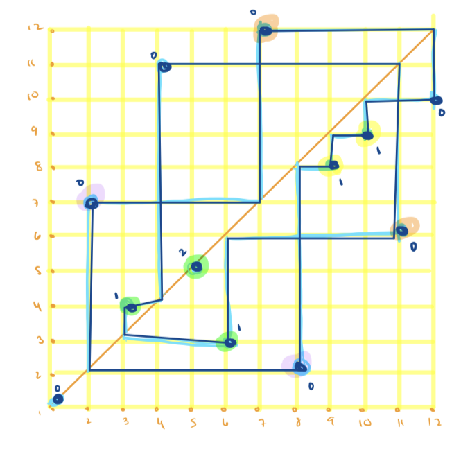
We begin by defining the maps and showing they each have $2^{n-1}$ fixed points. We first describe Corteel’s map [8] that applies the Foata-Zeilberger bijection to a permutation, then takes the complement of the resulting colored Motzkin path relative to the height of the path, and then applies the inverse Foata-Zeilberger bijection to find the corresponding permutation. To explain each step more precisely, we rely heavily on the nice visual explanation of the bijection between permutations and colored Motzkin paths via cycle diagrams given by Elizalde in [13].

Definition 6.1.

For a given permutation $\sigma$ , vertical lines on the cycle diagram connect the point $(i,i)$ to $(i,\sigma(i))$ , horizontal lines connect $(i,i)$ to $(\sigma^{-1}(i),i)$ (see Figure 1). Each vertex $(i,i)$ in the cycle diagram of $\sigma\in S_{n}$ can be classified into one of five types: an upward facing bracket , a downward facing bracket , a bounce from below , a bounce from above , or a fixed point . Using the notation for the Foata-Zeilberger bijection from the FindStat code for the Corteel map, we set $u=$ , $d=$ , $r=$ , and $b$ equal to either or . The letter $u$ corresponds to an up-step on the Motzkin path, $d$ a down-step, and $b$ and $r$ both correspond to a horizontal step.

The nesting number $p_{i}$ is the number of arcs in the cycle diagram containing the vertex $(i,\sigma(i)),$ where containment is defined from above if $(i,\sigma(i))$ is on or above the diagonal (i.e. if $(i,i)$ is associated with $u$ or $b$ ), and below if $(i,\sigma(i))$ is below the diagonal (i.e. if $(i,i)$ is associated with $r$ or $d$ ). More precisely,

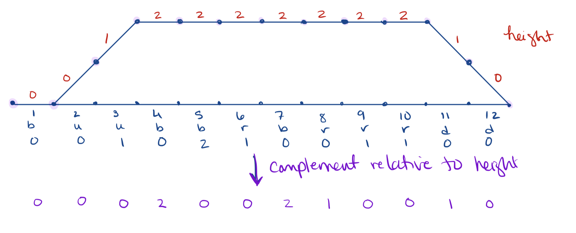
p_{i}=\begin{cases}\#\{j<i\ |\ \sigma(i)<\sigma(j)\}&(i,i)\mbox{ is associated with }u\mbox{ or }b,\\ \#\{i<j<n\ |\ \sigma(i)>\sigma(j)\}&(i,i)\mbox{ is associated with }r\mbox{ or }d.\end{cases}

The colored Motzkin path corresponding to $\sigma$ is completely described by a word-weight pair $(\mathbf{w},\mathbf{p})$ where $\mathbf{w}$ is the associated word of length $n$ in $\{u,d,r,b\}$ and $\mathbf{p}$ is the vector of non-negative integer weights (or colors) given by the associated nesting numbers $p_{i}$ .

Let $h_{i}$ denote the height of step $i$ in the corresponding Motzkin path, which is defined to be the height of the step’s lowest endpoint. The complement of $(\mathbf{w},\mathbf{p})$ is the colored Motzkin path corresponding to $(\mathbf{w},\mathbf{\bar{p}})$ where $\bar{p_{i}}=h_{i}-p_{i}-1$ if $w_{i}=r$ and $h_{i}-p_{i}$ otherwise (see Figure 2). The Corteel map (Map 239) sends $\sigma$ to the permutation found by applying the inverse Foata-Zeilberger bijection, i.e. the unique permutation whose cycle diagram corresponds to $(\mathbf{w},\mathbf{\bar{p}})$ .

Refer to caption — Figure 1. Cycle diagram for the permutation $\sigma=1~{}7~{}4~{}11~{}5~{}3~{}12~{}2~{}8~{}9~{}6~{}10$ . Each node $(i,\sigma(i))$ is labeled with $p_{i}$ , the number of cycles it is nested within in the cycle diagram. From this diagram we see that the corresponding word-weight pair for this $\sigma$ is $(\mathbf{w},\mathbf{p})=((b,u,u,b,b,r,b,r,r,r,d,d),(0,0,1,0,2,1,0,0,1,1,0,0)).$

One way to define the invert Laguerre heap map is to associate a heap of pieces, as in [41], to a given permutation by considering each decreasing run as one piece, beginning with the leftmost run. Two pieces commute if and only if the minimal element of one piece is larger than the maximal element of the other piece. The invert Laguerre heap map returns the permutation corresponding to the heap obtained by reversing the reading direction of the heap. We use an equivalent definition in terms of non-crossing arcs, as described in [24].

Definition 6.2.

Given a permutation $\sigma=\sigma_{1}\sigma_{2}\cdots\sigma_{n}$ , plot a point labeled $\sigma_{i}$ at $(i,\sigma_{i})$ , for each $1\leq i\leq n$ . For each decreasing run with more than one element in it, draw a line between each pair of adjacent numbers within the decreasing run. Now move all the points to be aligned vertically, converting the lines connecting numbers into non-crossing arcs, and keeping all numbers on the correct side of the arcs. The invert Laguerre heap map (Map 241) proceeds by vertically reflecting this arc diagram and reconstructing the permutation by applying the backward map.

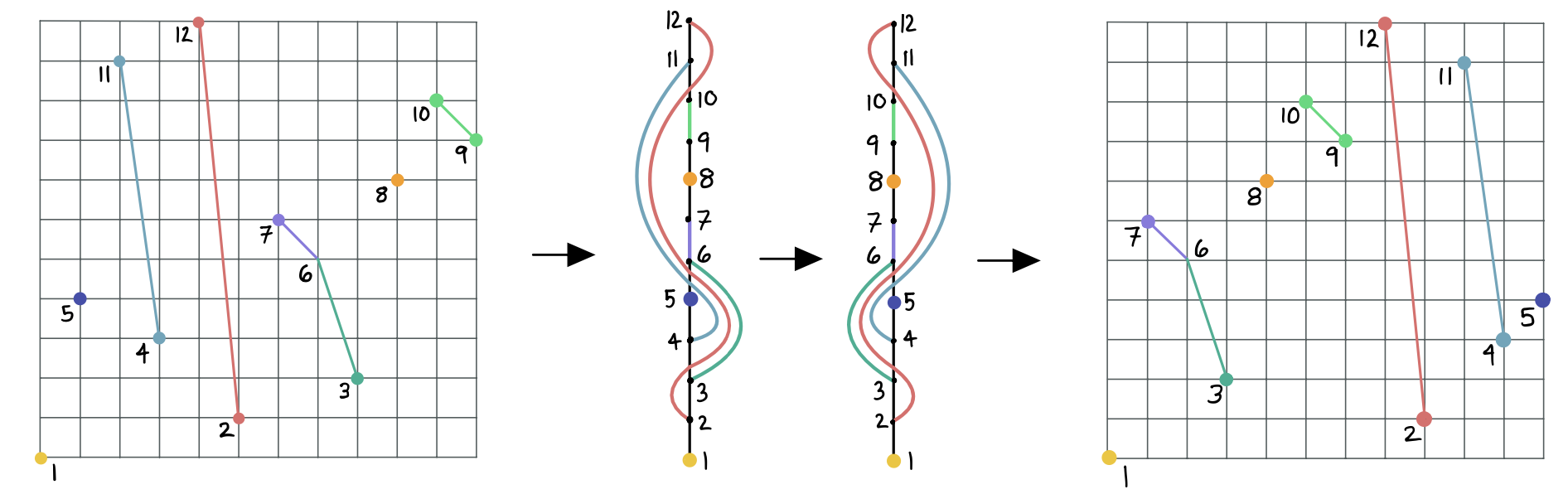
Example 6.3.

Consider $n=12$ and $\sigma=1~{}5~{}11~{}4~{}12~{}2~{}7~{}6~{}3~{}8~{}10~{}9$ , the output of the Corteel map from Figure 1. Applying the invert Laguerre heap map to $\sigma$ results in $1~{}7~{}6~{}3~{}8~{}10~{}9~{}12~{}2~{}11~{}4~{}5$ (see Figure 3). Since both the invert Laguerre heap and Corteel maps are involutions, comparing the output of the invert Laguerre heap map in this example to the starting permutation in Figure 1 shows these maps are not the same.

Note that applying the invert Laguerre heap map is not equivalent to recording the decreasing runs from right-to-left (preserving the order in each run), even though some examples may lead one to believe this.

Before proving our CSP theorems, we establish the number of fixed points of the Corteel and invert Laguerre heap maps in the following lemmas. We note that though the orbit structure of the maps match, the orbit elements differ. In particular, while there is a large overlap in the fixed points of each map, they are not all the same, and we thus have to prove the number of fixed points result separately.

Lemma 6.4.

The number of fixed points under the action of the Corteel map on $S_{n}$ is $2^{n-1}.$

Proof.

By definition, a fixed point of the Corteel map corresponds to a colored Motzkin path which is equal to its complement relative to the height of the path. Recall that the complement of $(\mathbf{w},\mathbf{p})$ is the colored Motzkin path corresponding to $(\mathbf{w},\mathbf{\bar{p}})$ where $\bar{p_{i}}=h_{i}-p_{i}-1$ if $w_{i}=r$ and $h_{i}-p_{i}$ otherwise. Thus, if the colored Motzkin path is fixed under the complement (i.e. $\mathbf{\bar{p}}=\mathbf{p}$ ) it must be that $h_{i}-1=2p_{i}$ when $w_{i}=r$ and $h_{i}=2p_{i}$ otherwise. Suppose $h_{i}=1.$ Since fractional values for $p_{i}$ are not allowed, it follows $w_{i}=r$ and the left endpoint of the $(i+1)$ -th step has height $1.$ By definition of the height function, $h_{i+1}$ must be less than or equal to 1. As the height at each step can only change by $0$ or $\pm 1$ , $h_{1}=0,$ and we just showed that if $h_{i}=1$ then $h_{i+1}\leq 1$ , it follows that at each step $h_{i}=0$ (and $w_{i}\in\{u,b,d\}$ ) or $h_{i}=1$ (and $w_{i}=r$ ), and in either case $p_{i}=\bar{p_{i}}=0.$

The only valid cycle diagrams satisfying these height conditions are those corresponding to words $\mathbf{w}$ which start with the letter $u$ or $b$ , end with the letter $b$ or $d$ , have an equal number of $u$ ’s and $d$ ’s, and for all $i>1$ satisfy the conditions:

•

$w_{i}\in\{u,b\}$ if and only if $w_{i-1}\in\{b,d\},$ and
•

$w_{i}\in\{r,d\}$ if and only if $w_{i-1}\in\{r,u\}.$

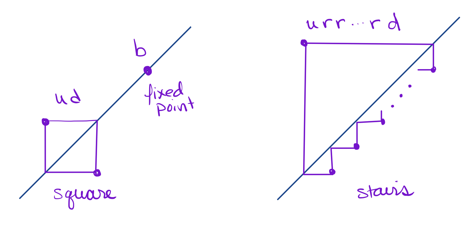
These conditions completely determine the last letter of the word $\mathbf{w}$ , but for each other letter we can choose between two possible values ( $\{u,b\}$ or $\{r,d\}$ ) depending on what letter precedes it. Thus there are $2^{n-1}$ possible words, and hence $2^{n-1}$ colored Motzkin paths fixed under the complement, and $2^{n-1}$ permutations fixed by the action of the Corteel map. ∎

From the preceding proof it follows that the permutations fixed by the Corteel map correspond to cycle diagrams made up of disjoint squares ( $ud$ pairs), stairs ( $urr\cdots rd$ ), and fixed points ( $b$ ). See Figure 4.

Lemma 6.5.

The number of fixed points under the action of the invert Laguerre heap map on $S_{n}$ is $2^{n-1}.$

Proof.

The invert Laguerre heap map corresponds to vertically flipping the arc diagrams of [24]. The arc diagrams that are fixed under this flip are the ones whose only arcs are between adjacent numbers. Each such arc can either be there or not, so the total number is $2^{n-1}$ . ∎

We will need the following statistic definitions as well as the definition of consecutive patterns from Definition 2.6.

Definition 6.6.

A crossing of a permutation $\sigma\in S_{n}$ is a pair $(i,j)$ such that either $i<j\leq\sigma(i)<\sigma(j)$ or $\sigma(i)<\sigma(j)<i<j$ . Using the cycle diagram described in Definition 6.1, the number of crossings of the permutation is the number of crossings of arcs in the diagram plus the number of times a line above the $y=x$ diagonal bounces off it.

A nesting of $\sigma$ is a pair $(i,j)$ such that $j<i\leq\sigma(i)<\sigma(j)$ or $\sigma(j)<\sigma(i)<i<j$ . In the cycle diagram, these are a pair of nested arcs above or below the $y=x$ diagonal, including the nesting of fixed points with respect to arcs above the diagonal. This is the sum of the nesting numbers $p_{i}$ from Definition 6.1.

As involutions, both the Corteel and invert Laguerre heap maps have orbits of size 1 or 2. Examining statistic values for each statistic over orbits of size 2, there was no clear pattern in the parity values of the statistic over the orbit. For example, while the fixed points of both maps have zero crossings and zero nestings, there are orbits of size 2 in which the number of crossings/nestings for both elements in the orbit have the same parity, and orbits in which they have opposite parity, and examples of each in which one element has zero crossings or zero nestings. Given we do not have a meaningful group representation view of these maps, this observation implies that proofs of CSP proceed by independently calculating the number of fixed points of the involution and comparing that to the value of the statistics generating function at $q=-1.$

Theorem 6.7.

The following statistics exhibit the CSP under the Corteel and invert Laguerre heap maps:

•

Statistic $39$ : The number of crossings,
•

Statistic $223$ : The number of nestings,
•

Statistic $356$ : The number of occurrences of the pattern $13-2$ ,
•

Statistic $358$ : The number of occurrences of the pattern $31-2$ .

Proof.

By [8, Theorem 2], the generating function for the number of crossings statistic is given by:

\sum_{k=1}^{n}\hat{E}_{k,n}(q)

where

\hat{E}_{k,n}(q)=q^{k-k^{2}}\sum_{i=0}^{k-1}(-1)^{i}[k-i]_{q}^{n}q^{k(i-1)}\left(\binom{n}{i}q^{k-i}+\binom{n}{i-1}\right).

By [42, Proposition 5.7], $\hat{E}_{k,n}(-1)=\binom{n-1}{k-1}$ , thus $\sum_{k=1}^{n}\hat{E}_{k,n}(-1)=\sum_{k=1}^{n}\binom{n-1}{k-1}=2^{n-1}$ . By Lemmas 6.4 and 6.5, this matches the number of fixed points of the Corteel and invert Laguerre heap maps, thus we have the desired CSP for statistic 39.

By [8, Proposition 4], the number of nestings of a permutation has the same generating function as the number of crossings, so the CSP holds for this statistic as well.

By [37, Corollary 30], the number of permutations of $n$ with $k-1$ descents and $m$ occurrences of the pattern $2-31$ is given by the coefficient of $q^{m}$ in $\hat{E}_{k,n}(q)$ . So the generating function for occurrences of the pattern $2-31$ is $\sum_{k=1}^{n}\hat{E}_{k,n}(q)$ , which is the generating function for the number of crossings given above. Applying the reverse map sends occurrences of the pattern $2-31$ to occurrences of the pattern $13-2$ , so we have that the number of occurrences of the pattern $13-2$ is equidistributed with the number of crossings. Thus the desired CSP holds.

Finally, $13-2$ patterns and $31-2$ patterns are related by the complement map and so are equidistributed. Thus we have the CSP for all four statistics. ∎

Note that FindStat indicates that the number of occurrences of the pattern $31-2$ and the number of crossings may be related by the Clark-Steingrimsson-Zeng map (Map 238) [7] followed by the inverse map. It may be interesting to prove the equidistribution of the number of $31-2$ patterns and crossings directly via these maps.

Definition 6.8.

A cycle descent of a permutation $\pi$ is a descent within a cycle of $\pi$ when $\pi$ is written in cycle notation with each cycle starting with its smallest element. The cycle descent number, denoted $\textnormal{cdes}(\pi)$ , counts the number of cycle descents in $\pi.$

Note that a cycle must have at least length $3$ to have a cycle descent; this is because the first number in a cycle is the smallest, so it does not form a cycle descent with the next number in the cycle.

Definition 6.9.

Given a permutation $\pi$ , a 12 arrow pattern, denoted $\underset{\tiny{1\shortrightarrow 2}}{\underline{12}}$ , is an instance of a $12-$ pattern, that is, an ascent $\pi_{i},\pi_{i+1}$ , with the special property that when you apply the first fundamental transform (Definition 2.4) to create a new permutation $\sigma=\mathcal{F}(\pi)$ , you have $\sigma(\pi_{i})=\pi_{i+1}$ .

See [5, Definition 17] for the definition of arrow patterns. Since this is a very special case, we do not need to define these in full generality.

Example 6.10.

Let $\pi=72358164$ . The following $(\pi_{1},\pi_{i+1})$ pairs form $12-$ patterns in $\pi:(2,3),(3,5),(5,8),$ and $(1,6)$ . To determine which of these are $\underset{\tiny{1\shortrightarrow 2}}{\underline{12}}$ arrow patterns, calculate the first fundamental transform of $\pi$ by inserting $)($ before each left-to-right maximum to divide $\pi$ into cycles. Writing the resulting permutation, $(7235)(8164),$ in one-line notation gives $\sigma=\mathcal{F}(\pi)=63587421.$ Since $\sigma(5)=7\not=8$ , $(5,8)$ does not form a $\underset{\tiny{1\shortrightarrow 2}}{\underline{12}}$ arrow pattern, but all other $12-$ pairs in this example do.

Note that a 12 pattern in a permutation $\pi$ given by $(\pi_{i},\pi_{i+1})$ is a 12 arrow pattern if $\pi_{i+1}$ is not a left-to-right maximum, and no left-to-right maximum can contribute to a 12 arrow pattern.

Lemma 6.11.

The following statistics are equidistributed:

•

Statistic $317$ : The cycle descent number,
•

Statistic $1744$ : The number of occurrences of the arrow pattern $\underset{\tiny{1\shortrightarrow 2}}{\underline{12}}$ .

Proof.

Let $\textnormal{Stat}1744(\pi)$ denote the number of occurrences of the arrow pattern $\underset{\tiny{1\shortrightarrow 2}}{\underline{12}}$ in $\pi$ .

We prove the first fundamental transform (see Definition 2.4), followed by the inverse map, is a bijection that maps Statistic 1744 to the number of cycle descents.

Let $\pi\in S_{n}$ and $\sigma$ denote the permutation obtained by applying the the first fundamental transform to $\pi$ . Let $a,b$ be an ascent of $\pi$ such that $\sigma(a)=b$ , i.e. an instance of a $\underset{\tiny{1\shortrightarrow 2}}{\underline{12}}$ arrow pattern. It must be that $b$ is not a left-to-right maximum of $\pi$ , since if it were, by definition of $\mathcal{F}$ , $a$ and $b$ would be in different cycles of $\sigma$ and it would not be true that $\sigma(a)=b$ . Thus, $a$ and $b$ are consecutive inside a cycle of $\sigma$ with the largest entry $c$ of that cycle written first. So the cycle looks like $(c,\ldots,a,b,\ldots,d)$ with $a<b<c$ and $d$ possibly equal to $b$ .

Having established that all instances of a $\underset{\tiny{1\shortrightarrow 2}}{\underline{12}}$ arrow pattern appear as consecutive elements in some cycle of $\sigma$ , we argue that the arrow pattern $a,b$ in $\pi$ corresponds to a unique cycle descent in $\sigma^{-1}$ , namely the cycle descent $c,d$ when $a$ is the smallest element in the cycle, and $b,a$ otherwise. To see this, take the inverse of $\sigma$ . This results in reversing everything after $c$ in the cycle, resulting in the cycle $(c,d,\ldots,b,a,\ldots)$ . To calculate the cycle descent number, we need to rewrite each cycle with the smallest number first. Let $s$ be this smallest element and suppose $a\not=s$ Then rewriting the cycle of $\sigma^{-1}$ so that $s$ appears first we have $(s,\ldots,b,a,\ldots)$ and $b,a$ is a cycle descent of $\sigma^{-1}$ .

If $s=a$ , then rewriting the cycle of $\sigma^{-1}$ so that it starts with the smallest element we have $(a,\ldots,c,d,\ldots,b)$ . In this case, $b,a$ is not a descent of $\sigma^{-1}$ , but $c,d$ is. And since $c$ was the first element, and maximal, in the cycle of $\sigma$ , it was not part of a $\underset{\tiny{1\shortrightarrow 2}}{\underline{12}}$ arrow pattern in $\pi.$ A similar argument in reverse shows that every cycle descent in $\sigma^{-1}$ that does not involve the maximal element corresponds directly to a $\underset{\tiny{1\shortrightarrow 2}}{\underline{12}}$ arrow patterns in $\pi$ , and a cycle descent in $\sigma^{-1}$ involving the maximal element corresponds to the $\underset{\tiny{1\shortrightarrow 2}}{\underline{12}}$ arrow patterns in $\pi$ involving the minimal cycle element. Thus every $\underset{\tiny{1\shortrightarrow 2}}{\underline{12}}$ arrow pattern contributing to Statistic 1744 on $\pi$ corresponds to a cycle descent of $\sigma^{-1}$ , and vice versa, establishing the result $\textnormal{Stat}1744(\pi)=\textnormal{cdes}(\sigma^{-1})$ .∎

Theorem 6.12.

The following statistics exhibit the CSP under the Corteel and invert Laguerre heap maps:

•

Statistic $317$ : The cycle descent number,
•

Statistic $1744$ : The number of occurrences of the arrow pattern $\underset{\tiny{1\shortrightarrow 2}}{\underline{12}}$ .

Proof.

Recall $\textnormal{cdes}(\pi)$ denotes the cycle descent number statistic on the permutation $\pi$ . By [19, Theorem 1] (setting $x=1$ and summing over all $i$ ), we have

\sum_{\pi\in\mathfrak{S}_{n}}(-1)^{\textnormal{cdes}(\pi)}t^{\pi^{-1}(1)}=2^{n-2}(t+t^{n}).

Setting $t=1$ gives that the generating function of the cycle descent number evaluated at $-1$ equals $2^{n-1}$ . Thus, the cycle descent number exhibits the desired CSP. Then by Lemma 6.11, the other statistic is equidistributed, completing the proof. ∎

We now give another equidistribution proof, which we will use to prove the CSP for these statistics. Again, recall Definition 2.6 for permutation patterns.

Lemma 6.13.

The following statistics are equidistributed:

•

Statistic $371$ : The number of midpoints of decreasing subsequences of length $3$ ,
•

Statistic $372$ : The number of midpoints of increasing subsequences of length $3$ ,
•

Statistic $1683$ : The number of distinct positions of the pattern letter $3$ in occurrences of $132$ ,
•

Statistic $1687$ : The number of distinct positions of the pattern letter $2$ in occurrences of $213$ .

Proof.

Take the pattern $132$ , in which we follow the entry that is initially the pattern letter $3$ . Its positions correspond to Statistic 1683. Write $1\,\leavevmode\hbox to11.37pt{\vbox to11.37pt{\pgfpicture\makeatletter\hbox{\hskip 5.68657pt\lower-5.68657pt\hbox to0.0pt{\pgfsys@beginscope\pgfsys@invoke{ }\definecolor{pgfstrokecolor}{rgb}{0,0,0}\pgfsys@color@rgb@stroke{0}{0}{0}\pgfsys@invoke{ }\pgfsys@color@rgb@fill{0}{0}{0}\pgfsys@invoke{ }\pgfsys@setlinewidth{0.4pt}\pgfsys@invoke{ }\nullfont\hbox to0.0pt{\pgfsys@beginscope\pgfsys@invoke{ } {{}}\hbox{\hbox{{\pgfsys@beginscope\pgfsys@invoke{ }{{}{{{}}}{{}}{}{}{}{}{}{}{}{}{}{{}\pgfsys@moveto{5.48657pt}{0.0pt}\pgfsys@curveto{5.48657pt}{3.03018pt}{3.03018pt}{5.48657pt}{0.0pt}{5.48657pt}\pgfsys@curveto{-3.03018pt}{5.48657pt}{-5.48657pt}{3.03018pt}{-5.48657pt}{0.0pt}\pgfsys@curveto{-5.48657pt}{-3.03018pt}{-3.03018pt}{-5.48657pt}{0.0pt}{-5.48657pt}\pgfsys@curveto{3.03018pt}{-5.48657pt}{5.48657pt}{-3.03018pt}{5.48657pt}{0.0pt}\pgfsys@closepath\pgfsys@moveto{0.0pt}{0.0pt}\pgfsys@stroke\pgfsys@invoke{ } }{{{{}}\pgfsys@beginscope\pgfsys@invoke{ }\pgfsys@transformcm{1.0}{0.0}{0.0}{1.0}{-2.5pt}{-3.22221pt}\pgfsys@invoke{ }\hbox{{\definecolor{pgfstrokecolor}{rgb}{0,0,0}\pgfsys@color@rgb@stroke{0}{0}{0}\pgfsys@invoke{ }\pgfsys@color@rgb@fill{0}{0}{0}\pgfsys@invoke{ }\hbox{{$3$}} }}\pgfsys@invoke{\lxSVG@closescope }\pgfsys@endscope}}} \pgfsys@invoke{\lxSVG@closescope }\pgfsys@endscope}}} \pgfsys@invoke{\lxSVG@closescope }\pgfsys@endscope{{{}}}{}{}\hss}\pgfsys@discardpath\pgfsys@invoke{\lxSVG@closescope }\pgfsys@endscope\hss}}\lxSVG@closescope\endpgfpicture}}\,2$ for this pattern, and the circled entry is the one that we follow. Through complement, inverse and complement again, this position is sent to the $2$ of the pattern $213$ :

1\,\leavevmode\hbox to11.37pt{\vbox to11.37pt{\pgfpicture\makeatletter\hbox{\hskip 5.68657pt\lower-5.68657pt\hbox to0.0pt{\pgfsys@beginscope\pgfsys@invoke{ }\definecolor{pgfstrokecolor}{rgb}{0,0,0}\pgfsys@color@rgb@stroke{0}{0}{0}\pgfsys@invoke{ }\pgfsys@color@rgb@fill{0}{0}{0}\pgfsys@invoke{ }\pgfsys@setlinewidth{0.4pt}\pgfsys@invoke{ }\nullfont\hbox to0.0pt{\pgfsys@beginscope\pgfsys@invoke{ } {{}}\hbox{\hbox{{\pgfsys@beginscope\pgfsys@invoke{ }{{}{{{}}}{{}}{}{}{}{}{}{}{}{}{}{{}\pgfsys@moveto{5.48657pt}{0.0pt}\pgfsys@curveto{5.48657pt}{3.03018pt}{3.03018pt}{5.48657pt}{0.0pt}{5.48657pt}\pgfsys@curveto{-3.03018pt}{5.48657pt}{-5.48657pt}{3.03018pt}{-5.48657pt}{0.0pt}\pgfsys@curveto{-5.48657pt}{-3.03018pt}{-3.03018pt}{-5.48657pt}{0.0pt}{-5.48657pt}\pgfsys@curveto{3.03018pt}{-5.48657pt}{5.48657pt}{-3.03018pt}{5.48657pt}{0.0pt}\pgfsys@closepath\pgfsys@moveto{0.0pt}{0.0pt}\pgfsys@stroke\pgfsys@invoke{ } }{{{{}}\pgfsys@beginscope\pgfsys@invoke{ }\pgfsys@transformcm{1.0}{0.0}{0.0}{1.0}{-2.5pt}{-3.22221pt}\pgfsys@invoke{ }\hbox{{\definecolor{pgfstrokecolor}{rgb}{0,0,0}\pgfsys@color@rgb@stroke{0}{0}{0}\pgfsys@invoke{ }\pgfsys@color@rgb@fill{0}{0}{0}\pgfsys@invoke{ }\hbox{{$3$}} }}\pgfsys@invoke{\lxSVG@closescope }\pgfsys@endscope}}} \pgfsys@invoke{\lxSVG@closescope }\pgfsys@endscope}}} \pgfsys@invoke{\lxSVG@closescope }\pgfsys@endscope{{{}}}{}{}\hss}\pgfsys@discardpath\pgfsys@invoke{\lxSVG@closescope }\pgfsys@endscope\hss}}\lxSVG@closescope\endpgfpicture}}\,2\xmapsto{\mathcal{C}}3\,\leavevmode\hbox to11.37pt{\vbox to11.37pt{\pgfpicture\makeatletter\hbox{\hskip 5.68657pt\lower-5.68657pt\hbox to0.0pt{\pgfsys@beginscope\pgfsys@invoke{ }\definecolor{pgfstrokecolor}{rgb}{0,0,0}\pgfsys@color@rgb@stroke{0}{0}{0}\pgfsys@invoke{ }\pgfsys@color@rgb@fill{0}{0}{0}\pgfsys@invoke{ }\pgfsys@setlinewidth{0.4pt}\pgfsys@invoke{ }\nullfont\hbox to0.0pt{\pgfsys@beginscope\pgfsys@invoke{ } {{}}\hbox{\hbox{{\pgfsys@beginscope\pgfsys@invoke{ }{{}{{{}}}{{}}{}{}{}{}{}{}{}{}{}{{}\pgfsys@moveto{5.48657pt}{0.0pt}\pgfsys@curveto{5.48657pt}{3.03018pt}{3.03018pt}{5.48657pt}{0.0pt}{5.48657pt}\pgfsys@curveto{-3.03018pt}{5.48657pt}{-5.48657pt}{3.03018pt}{-5.48657pt}{0.0pt}\pgfsys@curveto{-5.48657pt}{-3.03018pt}{-3.03018pt}{-5.48657pt}{0.0pt}{-5.48657pt}\pgfsys@curveto{3.03018pt}{-5.48657pt}{5.48657pt}{-3.03018pt}{5.48657pt}{0.0pt}\pgfsys@closepath\pgfsys@moveto{0.0pt}{0.0pt}\pgfsys@stroke\pgfsys@invoke{ } }{{{{}}\pgfsys@beginscope\pgfsys@invoke{ }\pgfsys@transformcm{1.0}{0.0}{0.0}{1.0}{-2.5pt}{-3.22221pt}\pgfsys@invoke{ }\hbox{{\definecolor{pgfstrokecolor}{rgb}{0,0,0}\pgfsys@color@rgb@stroke{0}{0}{0}\pgfsys@invoke{ }\pgfsys@color@rgb@fill{0}{0}{0}\pgfsys@invoke{ }\hbox{{$1$}} }}\pgfsys@invoke{\lxSVG@closescope }\pgfsys@endscope}}} \pgfsys@invoke{\lxSVG@closescope }\pgfsys@endscope}}} \pgfsys@invoke{\lxSVG@closescope }\pgfsys@endscope{{{}}}{}{}\hss}\pgfsys@discardpath\pgfsys@invoke{\lxSVG@closescope }\pgfsys@endscope\hss}}\lxSVG@closescope\endpgfpicture}}\,2\xmapsto{\mathcal{I}}\leavevmode\hbox to11.37pt{\vbox to11.37pt{\pgfpicture\makeatletter\hbox{\hskip 5.68657pt\lower-5.68657pt\hbox to0.0pt{\pgfsys@beginscope\pgfsys@invoke{ }\definecolor{pgfstrokecolor}{rgb}{0,0,0}\pgfsys@color@rgb@stroke{0}{0}{0}\pgfsys@invoke{ }\pgfsys@color@rgb@fill{0}{0}{0}\pgfsys@invoke{ }\pgfsys@setlinewidth{0.4pt}\pgfsys@invoke{ }\nullfont\hbox to0.0pt{\pgfsys@beginscope\pgfsys@invoke{ } {{}}\hbox{\hbox{{\pgfsys@beginscope\pgfsys@invoke{ }{{}{{{}}}{{}}{}{}{}{}{}{}{}{}{}{{}\pgfsys@moveto{5.48657pt}{0.0pt}\pgfsys@curveto{5.48657pt}{3.03018pt}{3.03018pt}{5.48657pt}{0.0pt}{5.48657pt}\pgfsys@curveto{-3.03018pt}{5.48657pt}{-5.48657pt}{3.03018pt}{-5.48657pt}{0.0pt}\pgfsys@curveto{-5.48657pt}{-3.03018pt}{-3.03018pt}{-5.48657pt}{0.0pt}{-5.48657pt}\pgfsys@curveto{3.03018pt}{-5.48657pt}{5.48657pt}{-3.03018pt}{5.48657pt}{0.0pt}\pgfsys@closepath\pgfsys@moveto{0.0pt}{0.0pt}\pgfsys@stroke\pgfsys@invoke{ } }{{{{}}\pgfsys@beginscope\pgfsys@invoke{ }\pgfsys@transformcm{1.0}{0.0}{0.0}{1.0}{-2.5pt}{-3.22221pt}\pgfsys@invoke{ }\hbox{{\definecolor{pgfstrokecolor}{rgb}{0,0,0}\pgfsys@color@rgb@stroke{0}{0}{0}\pgfsys@invoke{ }\pgfsys@color@rgb@fill{0}{0}{0}\pgfsys@invoke{ }\hbox{{$2$}} }}\pgfsys@invoke{\lxSVG@closescope }\pgfsys@endscope}}} \pgfsys@invoke{\lxSVG@closescope }\pgfsys@endscope}}} \pgfsys@invoke{\lxSVG@closescope }\pgfsys@endscope{{{}}}{}{}\hss}\pgfsys@discardpath\pgfsys@invoke{\lxSVG@closescope }\pgfsys@endscope\hss}}\lxSVG@closescope\endpgfpicture}}\,3\,1\xmapsto{\mathcal{C}}\leavevmode\hbox to11.37pt{\vbox to11.37pt{\pgfpicture\makeatletter\hbox{\hskip 5.68657pt\lower-5.68657pt\hbox to0.0pt{\pgfsys@beginscope\pgfsys@invoke{ }\definecolor{pgfstrokecolor}{rgb}{0,0,0}\pgfsys@color@rgb@stroke{0}{0}{0}\pgfsys@invoke{ }\pgfsys@color@rgb@fill{0}{0}{0}\pgfsys@invoke{ }\pgfsys@setlinewidth{0.4pt}\pgfsys@invoke{ }\nullfont\hbox to0.0pt{\pgfsys@beginscope\pgfsys@invoke{ } {{}}\hbox{\hbox{{\pgfsys@beginscope\pgfsys@invoke{ }{{}{{{}}}{{}}{}{}{}{}{}{}{}{}{}{{}\pgfsys@moveto{5.48657pt}{0.0pt}\pgfsys@curveto{5.48657pt}{3.03018pt}{3.03018pt}{5.48657pt}{0.0pt}{5.48657pt}\pgfsys@curveto{-3.03018pt}{5.48657pt}{-5.48657pt}{3.03018pt}{-5.48657pt}{0.0pt}\pgfsys@curveto{-5.48657pt}{-3.03018pt}{-3.03018pt}{-5.48657pt}{0.0pt}{-5.48657pt}\pgfsys@curveto{3.03018pt}{-5.48657pt}{5.48657pt}{-3.03018pt}{5.48657pt}{0.0pt}\pgfsys@closepath\pgfsys@moveto{0.0pt}{0.0pt}\pgfsys@stroke\pgfsys@invoke{ } }{{{{}}\pgfsys@beginscope\pgfsys@invoke{ }\pgfsys@transformcm{1.0}{0.0}{0.0}{1.0}{-2.5pt}{-3.22221pt}\pgfsys@invoke{ }\hbox{{\definecolor{pgfstrokecolor}{rgb}{0,0,0}\pgfsys@color@rgb@stroke{0}{0}{0}\pgfsys@invoke{ }\pgfsys@color@rgb@fill{0}{0}{0}\pgfsys@invoke{ }\hbox{{$2$}} }}\pgfsys@invoke{\lxSVG@closescope }\pgfsys@endscope}}} \pgfsys@invoke{\lxSVG@closescope }\pgfsys@endscope}}} \pgfsys@invoke{\lxSVG@closescope }\pgfsys@endscope{{{}}}{}{}\hss}\pgfsys@discardpath\pgfsys@invoke{\lxSVG@closescope }\pgfsys@endscope\hss}}\lxSVG@closescope\endpgfpicture}}\,1\,3.

Hence, the number of distinct positions of the pattern letter $3$ in $132$ is equidistributed with the number of distinct positions of the pattern letter $2$ in $213$ (Statistic 1637). The number of midpoints of increasing (resp. decreasing) subsequences of length $3$ corresponds to the patterns $1\,\leavevmode\hbox to11.37pt{\vbox to11.37pt{\pgfpicture\makeatletter\hbox{\hskip 5.68657pt\lower-5.68657pt\hbox to0.0pt{\pgfsys@beginscope\pgfsys@invoke{ }\definecolor{pgfstrokecolor}{rgb}{0,0,0}\pgfsys@color@rgb@stroke{0}{0}{0}\pgfsys@invoke{ }\pgfsys@color@rgb@fill{0}{0}{0}\pgfsys@invoke{ }\pgfsys@setlinewidth{0.4pt}\pgfsys@invoke{ }\nullfont\hbox to0.0pt{\pgfsys@beginscope\pgfsys@invoke{ } {{}}\hbox{\hbox{{\pgfsys@beginscope\pgfsys@invoke{ }{{}{{{}}}{{}}{}{}{}{}{}{}{}{}{}{{}\pgfsys@moveto{5.48657pt}{0.0pt}\pgfsys@curveto{5.48657pt}{3.03018pt}{3.03018pt}{5.48657pt}{0.0pt}{5.48657pt}\pgfsys@curveto{-3.03018pt}{5.48657pt}{-5.48657pt}{3.03018pt}{-5.48657pt}{0.0pt}\pgfsys@curveto{-5.48657pt}{-3.03018pt}{-3.03018pt}{-5.48657pt}{0.0pt}{-5.48657pt}\pgfsys@curveto{3.03018pt}{-5.48657pt}{5.48657pt}{-3.03018pt}{5.48657pt}{0.0pt}\pgfsys@closepath\pgfsys@moveto{0.0pt}{0.0pt}\pgfsys@stroke\pgfsys@invoke{ } }{{{{}}\pgfsys@beginscope\pgfsys@invoke{ }\pgfsys@transformcm{1.0}{0.0}{0.0}{1.0}{-2.5pt}{-3.22221pt}\pgfsys@invoke{ }\hbox{{\definecolor{pgfstrokecolor}{rgb}{0,0,0}\pgfsys@color@rgb@stroke{0}{0}{0}\pgfsys@invoke{ }\pgfsys@color@rgb@fill{0}{0}{0}\pgfsys@invoke{ }\hbox{{$2$}} }}\pgfsys@invoke{\lxSVG@closescope }\pgfsys@endscope}}} \pgfsys@invoke{\lxSVG@closescope }\pgfsys@endscope}}} \pgfsys@invoke{\lxSVG@closescope }\pgfsys@endscope{{{}}}{}{}\hss}\pgfsys@discardpath\pgfsys@invoke{\lxSVG@closescope }\pgfsys@endscope\hss}}\lxSVG@closescope\endpgfpicture}}\,{3}$ and $3\,\leavevmode\hbox to11.37pt{\vbox to11.37pt{\pgfpicture\makeatletter\hbox{\hskip 5.68657pt\lower-5.68657pt\hbox to0.0pt{\pgfsys@beginscope\pgfsys@invoke{ }\definecolor{pgfstrokecolor}{rgb}{0,0,0}\pgfsys@color@rgb@stroke{0}{0}{0}\pgfsys@invoke{ }\pgfsys@color@rgb@fill{0}{0}{0}\pgfsys@invoke{ }\pgfsys@setlinewidth{0.4pt}\pgfsys@invoke{ }\nullfont\hbox to0.0pt{\pgfsys@beginscope\pgfsys@invoke{ } {{}}\hbox{\hbox{{\pgfsys@beginscope\pgfsys@invoke{ }{{}{{{}}}{{}}{}{}{}{}{}{}{}{}{}{{}\pgfsys@moveto{5.48657pt}{0.0pt}\pgfsys@curveto{5.48657pt}{3.03018pt}{3.03018pt}{5.48657pt}{0.0pt}{5.48657pt}\pgfsys@curveto{-3.03018pt}{5.48657pt}{-5.48657pt}{3.03018pt}{-5.48657pt}{0.0pt}\pgfsys@curveto{-5.48657pt}{-3.03018pt}{-3.03018pt}{-5.48657pt}{0.0pt}{-5.48657pt}\pgfsys@curveto{3.03018pt}{-5.48657pt}{5.48657pt}{-3.03018pt}{5.48657pt}{0.0pt}\pgfsys@closepath\pgfsys@moveto{0.0pt}{0.0pt}\pgfsys@stroke\pgfsys@invoke{ } }{{{{}}\pgfsys@beginscope\pgfsys@invoke{ }\pgfsys@transformcm{1.0}{0.0}{0.0}{1.0}{-2.5pt}{-3.22221pt}\pgfsys@invoke{ }\hbox{{\definecolor{pgfstrokecolor}{rgb}{0,0,0}\pgfsys@color@rgb@stroke{0}{0}{0}\pgfsys@invoke{ }\pgfsys@color@rgb@fill{0}{0}{0}\pgfsys@invoke{ }\hbox{{$2$}} }}\pgfsys@invoke{\lxSVG@closescope }\pgfsys@endscope}}} \pgfsys@invoke{\lxSVG@closescope }\pgfsys@endscope}}} \pgfsys@invoke{\lxSVG@closescope }\pgfsys@endscope{{{}}}{}{}\hss}\pgfsys@discardpath\pgfsys@invoke{\lxSVG@closescope }\pgfsys@endscope\hss}}\lxSVG@closescope\endpgfpicture}}\,{1}$ respectively in the language above. Theorem $2$ of [40] states the equidistribution of $1\,\leavevmode\hbox to11.37pt{\vbox to11.37pt{\pgfpicture\makeatletter\hbox{\hskip 5.68657pt\lower-5.68657pt\hbox to0.0pt{\pgfsys@beginscope\pgfsys@invoke{ }\definecolor{pgfstrokecolor}{rgb}{0,0,0}\pgfsys@color@rgb@stroke{0}{0}{0}\pgfsys@invoke{ }\pgfsys@color@rgb@fill{0}{0}{0}\pgfsys@invoke{ }\pgfsys@setlinewidth{0.4pt}\pgfsys@invoke{ }\nullfont\hbox to0.0pt{\pgfsys@beginscope\pgfsys@invoke{ } {{}}\hbox{\hbox{{\pgfsys@beginscope\pgfsys@invoke{ }{{}{{{}}}{{}}{}{}{}{}{}{}{}{}{}{{}\pgfsys@moveto{5.48657pt}{0.0pt}\pgfsys@curveto{5.48657pt}{3.03018pt}{3.03018pt}{5.48657pt}{0.0pt}{5.48657pt}\pgfsys@curveto{-3.03018pt}{5.48657pt}{-5.48657pt}{3.03018pt}{-5.48657pt}{0.0pt}\pgfsys@curveto{-5.48657pt}{-3.03018pt}{-3.03018pt}{-5.48657pt}{0.0pt}{-5.48657pt}\pgfsys@curveto{3.03018pt}{-5.48657pt}{5.48657pt}{-3.03018pt}{5.48657pt}{0.0pt}\pgfsys@closepath\pgfsys@moveto{0.0pt}{0.0pt}\pgfsys@stroke\pgfsys@invoke{ } }{{{{}}\pgfsys@beginscope\pgfsys@invoke{ }\pgfsys@transformcm{1.0}{0.0}{0.0}{1.0}{-2.5pt}{-3.22221pt}\pgfsys@invoke{ }\hbox{{\definecolor{pgfstrokecolor}{rgb}{0,0,0}\pgfsys@color@rgb@stroke{0}{0}{0}\pgfsys@invoke{ }\pgfsys@color@rgb@fill{0}{0}{0}\pgfsys@invoke{ }\hbox{{$2$}} }}\pgfsys@invoke{\lxSVG@closescope }\pgfsys@endscope}}} \pgfsys@invoke{\lxSVG@closescope }\pgfsys@endscope}}} \pgfsys@invoke{\lxSVG@closescope }\pgfsys@endscope{{{}}}{}{}\hss}\pgfsys@discardpath\pgfsys@invoke{\lxSVG@closescope }\pgfsys@endscope\hss}}\lxSVG@closescope\endpgfpicture}}\,{3}$ and $1\,\leavevmode\hbox to11.37pt{\vbox to11.37pt{\pgfpicture\makeatletter\hbox{\hskip 5.68657pt\lower-5.68657pt\hbox to0.0pt{\pgfsys@beginscope\pgfsys@invoke{ }\definecolor{pgfstrokecolor}{rgb}{0,0,0}\pgfsys@color@rgb@stroke{0}{0}{0}\pgfsys@invoke{ }\pgfsys@color@rgb@fill{0}{0}{0}\pgfsys@invoke{ }\pgfsys@setlinewidth{0.4pt}\pgfsys@invoke{ }\nullfont\hbox to0.0pt{\pgfsys@beginscope\pgfsys@invoke{ } {{}}\hbox{\hbox{{\pgfsys@beginscope\pgfsys@invoke{ }{{}{{{}}}{{}}{}{}{}{}{}{}{}{}{}{{}\pgfsys@moveto{5.48657pt}{0.0pt}\pgfsys@curveto{5.48657pt}{3.03018pt}{3.03018pt}{5.48657pt}{0.0pt}{5.48657pt}\pgfsys@curveto{-3.03018pt}{5.48657pt}{-5.48657pt}{3.03018pt}{-5.48657pt}{0.0pt}\pgfsys@curveto{-5.48657pt}{-3.03018pt}{-3.03018pt}{-5.48657pt}{0.0pt}{-5.48657pt}\pgfsys@curveto{3.03018pt}{-5.48657pt}{5.48657pt}{-3.03018pt}{5.48657pt}{0.0pt}\pgfsys@closepath\pgfsys@moveto{0.0pt}{0.0pt}\pgfsys@stroke\pgfsys@invoke{ } }{{{{}}\pgfsys@beginscope\pgfsys@invoke{ }\pgfsys@transformcm{1.0}{0.0}{0.0}{1.0}{-2.5pt}{-3.22221pt}\pgfsys@invoke{ }\hbox{{\definecolor{pgfstrokecolor}{rgb}{0,0,0}\pgfsys@color@rgb@stroke{0}{0}{0}\pgfsys@invoke{ }\pgfsys@color@rgb@fill{0}{0}{0}\pgfsys@invoke{ }\hbox{{$3$}} }}\pgfsys@invoke{\lxSVG@closescope }\pgfsys@endscope}}} \pgfsys@invoke{\lxSVG@closescope }\pgfsys@endscope}}} \pgfsys@invoke{\lxSVG@closescope }\pgfsys@endscope{{{}}}{}{}\hss}\pgfsys@discardpath\pgfsys@invoke{\lxSVG@closescope }\pgfsys@endscope\hss}}\lxSVG@closescope\endpgfpicture}}\,{2}$ . Because $\mathcal{C}(1\,\leavevmode\hbox to11.37pt{\vbox to11.37pt{\pgfpicture\makeatletter\hbox{\hskip 5.68657pt\lower-5.68657pt\hbox to0.0pt{\pgfsys@beginscope\pgfsys@invoke{ }\definecolor{pgfstrokecolor}{rgb}{0,0,0}\pgfsys@color@rgb@stroke{0}{0}{0}\pgfsys@invoke{ }\pgfsys@color@rgb@fill{0}{0}{0}\pgfsys@invoke{ }\pgfsys@setlinewidth{0.4pt}\pgfsys@invoke{ }\nullfont\hbox to0.0pt{\pgfsys@beginscope\pgfsys@invoke{ } {{}}\hbox{\hbox{{\pgfsys@beginscope\pgfsys@invoke{ }{{}{{{}}}{{}}{}{}{}{}{}{}{}{}{}{{}\pgfsys@moveto{5.48657pt}{0.0pt}\pgfsys@curveto{5.48657pt}{3.03018pt}{3.03018pt}{5.48657pt}{0.0pt}{5.48657pt}\pgfsys@curveto{-3.03018pt}{5.48657pt}{-5.48657pt}{3.03018pt}{-5.48657pt}{0.0pt}\pgfsys@curveto{-5.48657pt}{-3.03018pt}{-3.03018pt}{-5.48657pt}{0.0pt}{-5.48657pt}\pgfsys@curveto{3.03018pt}{-5.48657pt}{5.48657pt}{-3.03018pt}{5.48657pt}{0.0pt}\pgfsys@closepath\pgfsys@moveto{0.0pt}{0.0pt}\pgfsys@stroke\pgfsys@invoke{ } }{{{{}}\pgfsys@beginscope\pgfsys@invoke{ }\pgfsys@transformcm{1.0}{0.0}{0.0}{1.0}{-2.5pt}{-3.22221pt}\pgfsys@invoke{ }\hbox{{\definecolor{pgfstrokecolor}{rgb}{0,0,0}\pgfsys@color@rgb@stroke{0}{0}{0}\pgfsys@invoke{ }\pgfsys@color@rgb@fill{0}{0}{0}\pgfsys@invoke{ }\hbox{{$2$}} }}\pgfsys@invoke{\lxSVG@closescope }\pgfsys@endscope}}} \pgfsys@invoke{\lxSVG@closescope }\pgfsys@endscope}}} \pgfsys@invoke{\lxSVG@closescope }\pgfsys@endscope{{{}}}{}{}\hss}\pgfsys@discardpath\pgfsys@invoke{\lxSVG@closescope }\pgfsys@endscope\hss}}\lxSVG@closescope\endpgfpicture}}\,{3})=3\,\leavevmode\hbox to11.37pt{\vbox to11.37pt{\pgfpicture\makeatletter\hbox{\hskip 5.68657pt\lower-5.68657pt\hbox to0.0pt{\pgfsys@beginscope\pgfsys@invoke{ }\definecolor{pgfstrokecolor}{rgb}{0,0,0}\pgfsys@color@rgb@stroke{0}{0}{0}\pgfsys@invoke{ }\pgfsys@color@rgb@fill{0}{0}{0}\pgfsys@invoke{ }\pgfsys@setlinewidth{0.4pt}\pgfsys@invoke{ }\nullfont\hbox to0.0pt{\pgfsys@beginscope\pgfsys@invoke{ } {{}}\hbox{\hbox{{\pgfsys@beginscope\pgfsys@invoke{ }{{}{{{}}}{{}}{}{}{}{}{}{}{}{}{}{{}\pgfsys@moveto{5.48657pt}{0.0pt}\pgfsys@curveto{5.48657pt}{3.03018pt}{3.03018pt}{5.48657pt}{0.0pt}{5.48657pt}\pgfsys@curveto{-3.03018pt}{5.48657pt}{-5.48657pt}{3.03018pt}{-5.48657pt}{0.0pt}\pgfsys@curveto{-5.48657pt}{-3.03018pt}{-3.03018pt}{-5.48657pt}{0.0pt}{-5.48657pt}\pgfsys@curveto{3.03018pt}{-5.48657pt}{5.48657pt}{-3.03018pt}{5.48657pt}{0.0pt}\pgfsys@closepath\pgfsys@moveto{0.0pt}{0.0pt}\pgfsys@stroke\pgfsys@invoke{ } }{{{{}}\pgfsys@beginscope\pgfsys@invoke{ }\pgfsys@transformcm{1.0}{0.0}{0.0}{1.0}{-2.5pt}{-3.22221pt}\pgfsys@invoke{ }\hbox{{\definecolor{pgfstrokecolor}{rgb}{0,0,0}\pgfsys@color@rgb@stroke{0}{0}{0}\pgfsys@invoke{ }\pgfsys@color@rgb@fill{0}{0}{0}\pgfsys@invoke{ }\hbox{{$2$}} }}\pgfsys@invoke{\lxSVG@closescope }\pgfsys@endscope}}} \pgfsys@invoke{\lxSVG@closescope }\pgfsys@endscope}}} \pgfsys@invoke{\lxSVG@closescope }\pgfsys@endscope{{{}}}{}{}\hss}\pgfsys@discardpath\pgfsys@invoke{\lxSVG@closescope }\pgfsys@endscope\hss}}\lxSVG@closescope\endpgfpicture}}\,{1}$ , the number of midpoints of decreasing sequences is also equidistributed with the statistics above. Thus Statistics $371$ and $372$ are also equidistributed. ∎

We now prove the following CSP theorem on the statistics from the above lemma and one additional related statistic, discussed at the end of the proof.

Theorem 6.14.

The following statistics exhibit the CSP under the Corteel and invert Laguerre heap maps:

•

Statistic $371$ : The number of midpoints of decreasing subsequences of length $3$ ,
•

Statistic $372$ : The number of midpoints of increasing subsequences of length $3$ ,
•

Statistic $1683$ : The number of distinct positions of the pattern letter $3$ in occurrences of $132$ in a permutation,
•

Statistic $1687$ : The number of distinct positions of the pattern letter $2$ in occurrences of $213$ ,
•

Statistic $1004$ : The number of indices that are either left-to-right maxima or right-to-left minima.

Proof.

We start by establishing the CSP result for Statistic 371: the number of midpoints of decreasing subsequences of length 3.

We define a map $\psi$ on $S_{n}$ that has the same orbit structure as the Corteel and invert Laguerre heap maps (meaning it is an involution with $2^{n-1}$ fixed points), where each fixed point contributes 0 to Statistic 371, and if $\sigma$ is not a fixed point then the number of midpoints of decreasing subsequences in $\sigma$ and $\psi(\sigma)$ differ by $\pm 1.$ To do so, let $3**$ denote a pattern of the form $321$ or $312$ . Let $j$ be the maximal midpoint index over all such patterns (if they exist), i.e. $j$ is maximal such that there exists $i,k$ with $i<j<k$ and $\sigma_{i}>\sigma_{j},\sigma_{k}$ . Thus $j$ is the maximum index corresponding to $2$ in $321$ patterns or $1$ in $312$ patterns. If $i<j<k$ and $i<j<k^{\prime}$ are both $3**$ patterns with $k<k^{\prime}$ then $i<k<k^{\prime}$ forms another $3**$ pattern with midpoint $k$ greater than $j$ . Thus, $3**$ patterns corresponding to maximum midpoint index $j$ have not only unique midpoint index $j$ , but also unique endpoint index $k$ .

We define $\psi$ as follows:

•

If $\sigma$ contains a $3**$ pattern, set $\psi(\sigma)$ to be the permutation created from $\sigma$ by swapping $\sigma_{j}$ and $\sigma_{k}$ . In other words, $\psi(\sigma)$ converts the $3**$ pattern with maximum midpoint index $j$ from $321$ to $312$ , or vice versa.
•

If $\sigma$ avoids the patterns $321$ and $312$ , then $\psi(\sigma)=\sigma$ .

Clearly, $\sigma$ is a fixed point of $\psi$ if and only if it avoids the patterns $321$ and $312$ . By [23], there are exactly $2^{n-1}$ such permutations of $[n]$ . Otherwise, by the definition of $\psi$ , the maximal midpoint index $j$ of a $3**$ pattern in $\sigma$ is the same as that in $\psi(\sigma),$ only $\psi(\sigma)_{j}$ corresponds to $1$ in the pattern if $\sigma_{j}$ corresponds to $2$ and $\psi(\sigma)_{j}$ corresponds to $2$ in the pattern if $\sigma_{j}$ corresponds to $1.$ Applying $\psi$ to $\psi(\sigma)$ swaps back the $312$ and $321$ patterns interchanged by $\psi$ . Thus $\psi(\psi(\sigma))=\sigma$ , establishing $\psi$ is an involution with the same orbit structure as the Corteel and invert Laguerre heap maps.

All that remains to show is that $\sigma$ and $\psi(\sigma)$ have a number of midpoints of decreasing subsequences of length $3$ that differ by $\pm 1$ . All decreasing subsequences of length three that do not involve $\sigma_{j}$ and $\sigma_{k}$ are unchanged by $\psi.$ Thus we only need to examine those patterns that include $\sigma_{j}$ , $\sigma_{k}$ , or both.

We start by noting that for all indices $s>j$ but not equal to $k$ , $\sigma_{s}>\sigma_{i}$ since otherwise $i,k,s$ would form a $3**$ pattern contradicting our assumption that $j$ was the maximal midpoint of such patterns. Thus, there are no decreasing subsequences of length 3 in $\sigma$ or $\psi(\sigma)$ starting at index $j$ or $k$ , or including index $k$ as a midpoint. Next consider length 3 decreasing subsequences in $\sigma$ with indices $i^{\prime}<j^{\prime}<k^{\prime},$ ending at $j$ or $k$ , i.e. with $k^{\prime}=j$ or $k.$ For all such subsequences, $j^{\prime}\leq j$ since otherwise $\sigma_{i^{\prime}},\sigma_{j^{\prime}},\sigma_{k^{\prime}}$ would form a $3**$ pattern with midpoint index $j^{\prime}$ greater than the maximum $j$ . If $j^{\prime}<j$ and $k^{\prime}=k$ or $j$ then swapping $\sigma_{j}$ and $\sigma_{k}$ exchanges the decreasing subsequence $\sigma_{i^{\prime}},\sigma_{j^{\prime}},\sigma_{k}$ with $\psi(\sigma)_{i^{\prime}},\psi(\sigma)_{j^{\prime}},\psi(\sigma)_{j}$ , or $\sigma_{i^{\prime}},\sigma_{j^{\prime}},\sigma_{j}$ with $\psi(\sigma)_{i^{\prime}},\psi(\sigma)_{j^{\prime}},\psi(\sigma)_{k}.$ In either case, $j^{\prime}$ is still a midpoint of a decreasing subsequence of length three and no length three subsequence midpoints have been added or destroyed.

The only length 3 decreasing subsequences left to consider are those with midpoint index $j$ . Recall that the endpoint index $k$ of a $3**$ pattern with maximum midpoint index $j$ is unique. Thus switching $\sigma_{j}$ and $\sigma_{k}$ either breaks all decreasing subsequences of length $3$ with midpoint index $j$ , or creates a decreasing subsequence of length 3 in $\psi(\sigma)$ with midpoint $j$ when $j$ was not a midpoint of such a decreasing subsequence before. More precisely, if $i<j<k$ are the indices of a $3**$ pattern in $\sigma$ , with $\sigma_{j}>\sigma_{k}$ , then $i,j,k$ forms a $321$ pattern in $\sigma$ that breaks in $\psi(\sigma)$ ; and if $\sigma_{j}<\sigma_{k}$ , then $i,j,k$ forms a $312$ pattern in $\sigma$ that becomes a $321$ pattern in $\psi(\sigma)$ . Thus, in swapping $\sigma_{j}$ and $\sigma_{k}$ , the number of midpoints of decreasing subsequences of length three is changed by $\pm 1.$

This shows that Statistic $371$ exhibits the CSP with respect to $\psi$ , and as $\psi$ has the same orbit structure as the Corteel and invert Laguerre heap maps, Statistic $371$ exhibits the CSP with respect to those maps as well.

Furthermore, Lemma 6.13 shows that Statistic $371$ is equidistributed with Statistics $372$ , $1683$ , and $1687$ . Finally, note that the generating function of Statistic $1004$ , the number of indices that are either left-to-right maxima or right-to-left minima, is the shifted reverse of Statistic $371$ . This is because Statistic $371$ consists of the indices that are neither left-to-right maxima nor right-to-left minima, so $\mathrm{Stat}371+\mathrm{Stat}1004=n$ and the CSP holds for this statistic as well. ∎

Example 6.15.

We’ll give an example of $\psi$ from the proof of Theorem 6.14. Let $n=6$ and $\sigma=251346$ . Then $\sigma$ has no midpoints of decreasing subsequences of length $3$ and $j=4,k=5$ since $\sigma_{4}=3,\sigma_{5}=4<\sigma_{2}=5$ . So, $\psi(\sigma)=251436$ , which has one midpoint of decreasing subsequences of length $3$ at spot $4$ .

Next, let $\sigma=352461$ . Then $\sigma$ has two midpoints of decreasing subsequences of length $3$ and $j=4,k=6$ since $\sigma_{4}=4,\sigma_{6}=1<\sigma_{2}=5$ . So, $\psi(\sigma)=352164$ , which has one midpoint of decreasing subsequences of length $3$ as it lost the one at spot $4$ .

We prove the following CSP by again defining and studying a new map with the same orbit structure. Recall Definition 2.6.

Theorem 6.16.

The following statistics exhibit the CSP under the Corteel and invert Laguerre heap maps:

•

Statistic $357$ : The number of occurrences of the pattern $12-3$ ,
•

Statistic $360$ : The number of occurrences of the pattern $32-1$ .

Proof.

We define a map $\psi$ on the set of permutations of $[n]$ that has the same orbit structure as the Corteel and invert Laguerre heap maps (meaning it is an involution with $2^{n-1}$ fixed points), where each fixed point contributes 0 to Statistic $360$ and the statistic for $\sigma$ and $\psi(\sigma)$ differs by $\pm 1$ when $\sigma$ is not a fixed point. Note that this is not the same map that was given in the proof of Theorem 6.14.

For $n\leq 2$ , define $\psi$ as the identity map. For $n=3$ , define $\psi$ as pairing $312$ to $321$ and mapping everything else to itself.

For $n>3$ , define $\psi$ as follows:

•

If $\sigma_{1}\neq 1,2$ , $\psi(\sigma)$ is formed from $\sigma$ by swapping the values $1$ and $2$ .
•

If $\sigma_{1}=1$ or $\sigma_{1}=2$ , let $\sigma^{\prime}$ be the permutation of $[n-1]$ defined by $\sigma^{\prime}_{i}=\sigma_{i+1}-1$ if $\sigma_{i+1}\neq 1$ and $\sigma^{\prime}_{i}=1$ otherwise. Define $\psi(\sigma)$ by setting $\psi(\sigma)_{1}=\sigma_{1}$ . If $\sigma_{1}=1$ , for $i>1$ , $\psi(\sigma)_{i}=\psi(\sigma^{\prime})_{i-1}+1$ . If $\sigma_{1}=2,$ for $i>1$ , $\psi(\sigma)_{i}=\psi(\sigma^{\prime})_{i-1}+1$ if $\psi(\sigma^{\prime})_{i-1}\neq 1$ and $\psi(\sigma)_{i}=1$ otherwise.

Then $\psi$ is an involution. The number of fixed points for $n\leq 3$ is $2^{n-1}$ . For $n>3$ , the number of fixed points is $2$ times the number of fixed points for $n-1$ , so again we have $2^{n-1}$ . In addition, one can verify that any fixed point for $n\leq 3$ contributes 0 to the statistic. For $n>3$ , any fixed point has $\sigma_{1}=1$ or $2$ so $\sigma_{1}$ contributes to no pattern of the form $32-1$ . Thus, any occurrence of that pattern must come from $\sigma_{2}\sigma_{3}\dotsm\sigma_{n}$ . But as $\sigma$ is a fixed point $\sigma^{\prime}$ must also be a fixed point, so $\sigma_{2}\sigma_{3}\dotsm\sigma_{n}$ contributes 0 to the statistic.

Lastly, we show that over any orbit of size $2$ , the change in the statistic is $\pm 1$ . For simplicity, say $(jk,l)$ contributes to the statistic if they have the pattern $32-1$ , that is if the values $j,k,$ and $l$ occur in that order in the permutation and have $j>k>l$ with $k$ following directly after $j$ . For example, $(32,1)$ contributes to the statistic for $\sigma=3241$ and $(42,1)$ in $\sigma=4231$ .

For $n\leq 2$ , all orbits are of size $1$ , so there is nothing to show. For $n=3$ , the only orbit of size $2$ is $\{321,312\}$ , which we can verify has a change in the statistic of $\pm 1$ . For $\sigma$ in an orbit of size $2$ , either $2$ and $1$ are swapped in $\sigma$ or either $\sigma_{1}=1$ or $\sigma_{1}=2$ and $1$ and $2$ are swapped in some $\sigma^{\prime},\sigma^{\prime\prime},\dotsc$ So, we show for $n\geq 3$ that swapping $1$ and $2$ in $\sigma$ contributes $\pm 1$ to the statistic and then use induction for the cases $\sigma_{1}=1$ and $\sigma_{1}=2$ , as $\sigma_{1}$ does not contribute to any occurrences of the pattern.

If $(j2,1)$ contributes to the statistic, then swapping $1$ and $2$ changes the order of $1$ and $2$ and thus removes one occurrence of the pattern $32-1$ . As $2$ moves to the right, any triple of the form $(jk,2)$ still contributes to the pattern in $\psi(\sigma)$ , and any new triples $(jk,2)$ contributing to the statistic in $\psi(\sigma)$ would have been contributing as $(jk,1)$ in $\sigma$ . If $(jk,1)$ contributes to the statistic in $\sigma$ , then it either remains in $\psi(\sigma)$ (if $1$ is still to the right of $k$ after the swap) or it becomes $(jk,2)$ in $\psi(\sigma)$ (if $1$ is to the left of $k$ after the swap). There can be no new contributions of the form $(jk,1)$ in $\psi(\sigma)$ as $1$ moved to the left. Thus, the change in the total number of occurrences of the pattern $32-1$ is $-1$ .

If instead $1$ is to the left of $2$ in the statistic, then switching $1$ and $2$ adds $(j2,1)$ as an occurrence of the pattern $32-1$ in $\psi(\sigma)$ . Any triple of the form $(jk,2)$ in $\sigma$ either remains in $\psi(\sigma)$ (if $2$ is still to the right of $k$ after the swap) or becomes $(jk,1)$ in $\psi(\sigma)$ (if $2$ is to the left of $k$ after the swap). There can be no new contributions of the form $(jk,2)$ in $\psi(\sigma)$ as $2$ moved to the left. Any triple of the form $(jk,1)$ in $\sigma$ remains in $\psi(\sigma)$ as $1$ moved to the right, and any new triples $(jk,1)$ contributing to the statistic in $\psi(\sigma)$ would have been contributing as $(jk,2)$ in $\sigma$ . Thus, the change in the total number of occurrences of the pattern $32-1$ is $1$ .

Each instance of a $32-1$ pattern invertibly transforms to a $12-3$ pattern by the complement map, thus the CSP holds for the number of occurrences of the pattern $12-3$ also. ∎

Example 6.17.

We’ll give an example of $\psi$ from the proof of Theorem 6.16. Let $n=4$ and $\sigma=1432$ . Since $\sigma_{1}=1$ we must look at $\sigma^{\prime}=321$ a permutation of $[3]$ . $\psi(321)=312$ , so $\psi(1432)=1423$ . The number of occurrences of the pattern $32-1$ is $1$ for $\sigma$ and 0 for $\psi(\sigma)$ .

On the other hand, if we consider $\sigma=1342$ , then $\sigma^{\prime}=231$ . Then $\psi(\sigma^{\prime})=231$ , so $\psi(\sigma)=1342$ , and $\sigma$ is a fixed point.

We leave the following as conjectures. They have been tested up to $n=10$ .

Conjecture 6.18.

The difference in Coxeter length of a permutation and its image under the Simion-Schmidt map (Statistic $123$ ) exhibits the CSP under the Corteel and invert Laguerre heap maps.

Conjecture 6.19.

The number of weak exceedances that are also mid-points of a decreasing subsequence of length $3$ (Statistic $373$ ) is equidistributed with the cycle descent number (Statistic $317$ ) and thus exhibits the CSP under the Corteel and invert Laguerre heap maps.

7. Alexandersson-Kebede map (Map 257)

The Alexandersson-Kebede map $\kappa$ is an involution on permutations that preserves right-to-left minima. It was introduced in [2] to give a bijective proof of an identity regarding derangements and to refine it with respect to right-to-left minima.

In this section, we prove the following statistics exhibit the CSP with respect to this map.

•

Theorem 7.4: The sum of the numbers of left-to-right maxima and right-to-left minima
•

Corollary 7.7 (Statistic 1005): The number of indices that are either left-to-right maxima or right-to-left minima but not both
•

Theorem 7.10 (Statistic $1727$ ): The number of invisible inversions.

Definition 7.1.

Let $\sigma\in S_{n}.$ The Alexandersson-Kebede map $\kappa$ is defined as follows. Let $i$ be the smallest odd integer such that $\sigma\cdot(i,i+1)$ and $\sigma$ have the same set of right-to-left minima, if such an $i$ exists. If it does not, then $\kappa(\sigma)=\sigma$ . Otherwise, $\kappa(\sigma)=\sigma\cdot(i,i+1)$ .

Proposition 7.2 (Lemma 4.1.3 of [2]).

The map $\kappa$ satisfies the following:

•

$\kappa$ is an involution.
•

$\kappa$ preserves the number of right-to-left minima.
•

The fixed points of $\kappa$ are permutations satisfying $\{\sigma(i),\sigma(i+1)\}=\{i,i+1\}$ for all odd $i$ . These are called decisive permutations in [2].
•

There are $2^{\lfloor\frac{n}{2}\rfloor}$ fixed points.

Example 7.3.

Consider the permutation $\sigma=2134756$ . Its right-to-left minima are $\{1,3,4,5,6\}$ . To find $\kappa(\sigma)$ , we need to find the smallest odd $i$ for which $\sigma\cdot(i,i+1)$ and $\sigma$ have the same right-to-left minima. We cannot choose $i=1$ since $\sigma\cdot(1,2)=1234756$ makes $2$ a right-to-left minimum. We cannot choose $i=3$ since $\sigma\cdot(3,4)=2143756$ makes $4$ not a right-to-left minimum anymore. Then $i=5$ since $2134756$ and $2134576$ have the same set of right-to-left minima. Here, $\kappa(\sigma)=2134576$ .

Our first theorem regarding this map is given below. We then use it in Corollary 7.7 to prove the CSP for a statistic in FindStat.

Theorem 7.4.

The statistic given as the sum of the numbers of left-to-right maxima and right-to-left minima exhibits the cyclic sieving phenomenon with respect to the Alexandersson-Kebede map.

Before proving Theorem 7.4, we need a few lemmas.

Lemma 7.5.

When $\sigma\in S_{n}$ is not fixed by $\kappa,$ the number of left-to-right maxima for $\sigma$ and for $\kappa(\sigma)$ differ by one.

Proof.

Let $\sigma\in S_{n}$ so that $\kappa$ does not fix $\sigma.$ Then there exists a smallest odd integer $i$ so that the right-to-left minima of $\sigma$ are equal to the right-to-left minima of $\kappa(\sigma).$ Note that for all odd integers $j<i,$ the sets of right-to-left minima for $\sigma(j~{}j+1)$ and $\sigma$ are different. Thus, either $\sigma(j),\sigma(j+1),$ or both are right-to-left minima for all odd integers $j<i,$ which means $\sigma(i)$ and $\sigma(i+1)$ are greater than $\sigma(j)$ and $\sigma(j+1)$ for all odd $j<i.$ Then either $\sigma(i)>\sigma(i+1)$ or $\sigma(i)<\sigma(i+1).$ If $\sigma(i)>\sigma(i+1),$ then only $\sigma(i)$ is a left-to-right maximum. If $\sigma(i)<\sigma(i+1),$ then both $\sigma(i)$ and $\sigma(i+1)$ are left-to-right maxima. So, under the action of $\kappa$ we have $\sigma(i~{}i+1)$ , meaning that over one orbit, the number of left-to-right maxima differs by one. ∎

Lemma 7.6.

The number of left-to-right maxima and the number of right-to-left minima are equal for permutations fixed under $\kappa$ .

Proof.

Recall from Proposition 7.2 that the fixed points of $\kappa$ are permutations satisfying $\{\sigma(i),\sigma(i+1)\}=\{i,i+1\}$ for all odd $i$ . We prove that, for each pair $\{i,i+1\}$ with odd $i$ , either only one of them is a left-to-right maximum and the other one is a right-to-left minimum, or that both of them are left-to-right maxima and right-to-left minima.

For a permutation $\sigma$ fixed under $\kappa$ and a pair $\{i,i+1\}$ with odd $i$ , we know that all entries to the left of $i$ and $i+1$ are smaller, and that all entries to the right of $i$ and $i+1$ are larger. Hence, there is at least one left-to-right maximum and one right-to-left minimum among $\{i,i+1\}$ .

If $\sigma(i)=i$ (and $\sigma(i+1)=i+1$ ), there are two left-to-right maxima and two right-to-left minima. If $\sigma(i+1)=i$ (and $\sigma(i)=i+1$ ), then only $\sigma(i+1)$ is a right-to-left minimum, and $\sigma(i)$ is a left-to-right maximum. Either way, the number of left-to-right maxima is the same as the number of right-to-left minima for permutations that are fixed under $\kappa$ . ∎

Proof of Theorem 7.4.

Since $\kappa$ is an involution, we only need to show that the statistic-generating function evaluated at $q=-1$ gives the number of fixed points. By Proposition 7.2, this is $2^{\lfloor\frac{n}{2}\rfloor}$ .

Let Stat be the statistic counting the sum of the numbers of right-to-left minima and left-to-right maxima. Then, we need to show that

\sum_{\sigma\in S_{n}}(-1)^{\textnormal{Stat}(\sigma)}=2^{\lfloor\frac{n}{2}\rfloor}.

We break the sum above into two parts, to account for the fixed points separately:

(1)

\sum_{\sigma\in S_{n}}(-1)^{\textnormal{Stat}(\sigma)}=\sum_{\begin{subarray}{c}\sigma\in S_{n}\\ \kappa(\sigma)=\sigma\end{subarray}}(-1)^{\textnormal{Stat}(\sigma)}+\sum_{\begin{subarray}{c}\sigma\in S_{n}\\ \kappa(\sigma)\neq\sigma\end{subarray}}(-1)^{\textnormal{Stat}(\sigma)}.

We know from Proposition 7.2 and Lemma 7.5 that

\sum_{\begin{subarray}{c}\sigma\in S_{n}\\ \kappa(\sigma)\neq\sigma\end{subarray}}(-1)^{\textnormal{Stat}(\sigma)}=\sum_{\text{orbits of }\kappa}((-1)+1)=0.

Furthermore, when we write L2R and R2L for left-to-right and right-to-left, respectively, Lemma 7.6 tells us that

\sum_{\begin{subarray}{c}\sigma\in S_{n}\\ \kappa(\sigma)=\sigma\end{subarray}}(-1)^{\#\text{L2R maxima}(\sigma)+\#\text{R2L minima}(\sigma)}=\sum_{\begin{subarray}{c}\sigma\in S_{n}\\ \kappa(\sigma)=\sigma\end{subarray}}\underbrace{(-1)^{2\#\text{L2R maxima}(\sigma)}}_{1}=\#\{\sigma\in S_{n}\mid\sigma=\kappa(\sigma)\}=2^{\lfloor\frac{n}{2}\rfloor}.

Hence, Equation (1) becomes

\sum_{\begin{subarray}{c}\sigma\in S_{n}\\ \kappa(\sigma)=\sigma\end{subarray}}(-1)^{\textnormal{Stat}(\sigma)}+\sum_{\begin{subarray}{c}\sigma\in S_{n}\\ \kappa(\sigma)\neq\sigma\end{subarray}}(-1)^{\textnormal{Stat}(\sigma)}=2^{\lfloor\frac{n}{2}\rfloor}+0,

which is exactly the number of fixed points under $\kappa$ . This shows that the map exhibits the cyclic sieving phenomenon for the sum of the numbers of left-to-right maxima and right-to-left minima. ∎

Corollary 7.7.

The number of indices of a permutation that are either left-to-right maxima or right-to-left minima but not both (Statistic 1005), exhibits the cyclic sieving phenomenon for the Alexandersson-Kebede map.

Proof.

This follows from Theorem 7.4. Since the map is an involution, we prove the cyclic sieving phenomenon by evaluating the statistic-generating function at $q=-1$ . This means that only the parity of the statistic matters. To calculate the number of indices for a permutation that are either left-to-right maxima or right-to-left minima but not both, we subtract an even number from the sum of the numbers of left-to-right maxima and right-to-left minima, meaning that the statistics, for each permutation, always have the same parity. Thus, the cyclic sieving phenomenon also holds for the number of indices for a permutation that are either left-to-right maxima or right-to-left minima but not both with respect to the the Alexandersson-Kebede map. ∎

We now define the second FindStat statistic we show exhibits the CSP with respect to $\kappa$ .

Definition 7.8.

An inversion $(i,j)$ of $\sigma$ is said to be invisible if it satisfies $\sigma(i)>\sigma(j)>i$ .

Lemma 7.9.

Fixed points under $\kappa$ have no invisible inversion.

Proof.

Assume $\sigma\in S_{n}$ is fixed by $\kappa$ and suppose there exists a pair $j>k$ such that $\sigma(k)>\sigma(j)>k.$ Since $\kappa\sigma=\sigma,$ then from Proposition 7.2 either $\sigma(k)=k$ or $\sigma(k)=k+1$ and $\sigma(j)=j$ or $\sigma(j)=j+1.$ In any combination we get a contradiction that $\sigma(k)>\sigma(j)>k.$ ∎

Theorem 7.10.

The number of invisible inversions (Statistic $1727$ ) exhibits the cyclic sieving phenomenon with respect to the Alexandersson-Kebede map.

Proof.

To show that the number of invisible inversions exhibits the CSP under $\kappa$ , we define a new involution $\psi:S_{n}\rightarrow S_{n}$ with $2^{\lfloor\frac{n}{2}\rfloor}$ fixed points; see Example 7.11. We show the fixed points of $\psi$ have no invisible inversions, and orbits of size $2$ are made of two permutations whose number of invisible inversions differs by $\pm 1$ . Showing that the number of invisible inversions exhibits the CSP under $\psi$ amounts to showing the CSP for the statistics under the Alexandersson-Kebede map, since the orbit structure is the same.

Define $\psi:S_{n}\rightarrow S_{n}$ as follows.

•

If $n$ is even, section the permutation into blocks of size $2$ by grouping the spots $i$ and $i+1$ with $i$ odd. If there is some pair of values $(i,i+1)$ with $i$ odd where $i$ and $i+1$ are not both in the $\frac{i+1}{2}$ block, pick $i$ to be maximal and define $\psi(\sigma)$ to be the involution swapping the values $i$ and $i+1$ .
•

If $n$ is odd, place $1$ in its own block and section the remainder of the permutation into blocks of size $2$ by grouping spots $i$ and $i+1$ with $i$ even. If there is some pair of values $(i,i+1)$ with $i$ even where $i$ and $i+1$ are not both in the $\frac{i}{2}+1$ block, pick $i$ to be maximal and define $\psi(\sigma)$ by swapping the values $i$ and $i+1$ .

Let $\sigma$ be a permutation not fixed by $\psi$ and let $(i,i+1)$ be the swapped pair. We show that swapping $i$ and $i+1$ either breaks or creates an invisible inversion with those values. Consider $j,k$ such that $1\leq j,k\leq n$ , $\sigma_{j}=i$ , $\sigma_{k}=i+1$ . Then $\{j,k\}\neq\{i,i+1\}$ . As $i$ is chosen to be maximal, we have $j,k\leq i+1$ since every value greater than $i+1$ must already be in its assigned block to the right of spot $i+1$ . Similarly, for all $t\leq i+1$ , we have $\sigma_{t}\leq i+1$ .

If $j<k$ , then $\sigma_{j}=i$ cannot be in its block, so $j<i$ . Thus, $\psi(\sigma)_{j}=\sigma_{k}=i+1>\psi(\sigma)_{k}=\sigma_{j}=i>j,$ so $(j,k)$ is an invisible inversion of $\psi(\sigma)$ but not in $\sigma$ because $\sigma_{j}=i<\sigma_{k}=i+1$ . If $k<j$ , then $\sigma_{k}=i+1$ cannot be in its block, so $k<i$ . Thus, $\sigma_{k}=i+1>\sigma_{j}=i>k$ , so $(k,j)$ is an invisible inversion of $\sigma$ but not in $\psi(\sigma)$ since $\psi(\sigma)_{k}=\sigma_{j}=i<\psi(\sigma)_{j}=\sigma_{k}=i+1$ .

Additionally, swapping these values does not create or break any other invisible inversions. First, note that any invisible inversion not involving spots $j$ and $k$ is unaffected by this map, so we only need to consider invisible inversions involving either spot $j$ or spot $k$ . Let $\sigma_{t}\neq i,i+1$ . Recall that if $t\leq i+1$ , then $\sigma_{t}\leq i+1$ , so since $\sigma_{t}\neq i,i+1$ , if $t\leq i+1$ , then $\sigma_{t}<i$ . Hence there are no inversions of the form $(t,j)$ or $(t,k)$ . Thus, there are two cases to check.

•

If $(j,t)$ is an invisible inversion in $\sigma$ , then $j<t$ and $\sigma_{j}=i>\sigma_{t}>j$ . Then $\psi(\sigma)_{j}=i+1>\sigma_{t}>j$ and $(j,t)$ is an invisible inversion in $\psi(\sigma)$ . Similarly, if $(j,t)$ is an invisible inversion in $\psi(\sigma)$ , then $\psi(\sigma)_{j}=i+1>\psi(\sigma)_{t}=\sigma_{t}>j$ and as $\sigma_{t}\neq i$ , $\sigma_{j}=i>\sigma_{t}>j$ and $(j,t)$ is an invisible inversion in $\sigma$ .
•

If $(k,t)$ is an invisible inversion in $\sigma$ , then $k<t$ and $\sigma_{k}=i+1>\sigma_{t}>k$ . As $\sigma_{t}\neq i$ , then $\psi(\sigma)_{k}=i>\sigma_{t}>k$ and $(k,t)$ is an invisible inversion in $\psi(\sigma)$ . Similarly, if $(k,t)$ is an invisible inversion in $\psi(\sigma)$ , then $\psi(\sigma)_{k}=\sigma_{j}=i>\psi(\sigma)_{t}=\sigma_{t}>k$ , so $\sigma_{k}=i+1>\sigma_{t}>k$ and $(k,t)$ is an invisible inversion in $\sigma$ .

Let $F$ be the set of fixed points of $\psi$ . If $n$ is even, then $F$ is equal to the set of fixed points of $\kappa$ . So when $n$ is even, $\psi$ is a map with the same orbit structure as $\kappa$ , the same fixed points as $\kappa$ (which contribute 0 to the number of invisible inversions), and such that the number of invisible inversions changes by $\pm 1$ over each orbit of size $2$ . As the number of invisible inversions exhibits the CSP on $\psi$ , it also exhibits the CSP on $\kappa$ .

If $n$ is odd, then the fixed points of $\kappa$ are not the same as the fixed points of $\psi$ , but the two sets are equinumerous, as the fixed points of $\psi$ are exactly those $\sigma$ with $\sigma_{1}=1$ and all other pairs in their blocks. Additionally, each fixed point has no invisible inversion, and the number of invisible inversions changes by $\pm 1$ over each orbit. Thus, the statistic exhibits the CSP under $\psi$ . Therefore, as the number of invisible inversions exhibits the CSP on $\psi$ , it also exhibits the CSP on $\kappa$ . ∎

Example 7.11.

Let $n=8$ . Then $\sigma=21534687$ maps to $\psi(\sigma)=21634587$ . Since $7$ and $8$ are already in the correct block, we switched $5$ and $6$ . There is one invisible inversion in $\sigma$ , $(3,5)$ , and two invisible inversions in $\psi(\sigma)$ , $(3,5)$ and $(3,6)$ . In this case, $21345687$ is a fixed point.

Next, let $n=9$ . Then $\sigma=215346879$ maps to $\psi(\sigma)=215346978$ . There is one invisible inversion in $\sigma$ , $(3,5)$ , and two invisible inversions in $\psi(\sigma)$ , $(3,5)$ and $(7,9)$ . In this case, $215346879$ is not a fixed point, but $132456789$ is a fixed point.

8. Conjugation by the long cycle (Map 265)

Conjugation by the long cycle $(1,2,\ldots,n)$ has orbits of several different lengths. Specifically, the lengths of the orbits are all the divisors of $n$ . Therefore, proofs of the cyclic sieving phenomenon are more involved and often use representation theory. Running the experiment to search for occurrences of cyclic sieving, we noticed that the only statistics in FindStat that could exhibit the phenomenon had one of three generating functions. Here, we present equidistribution results and give references to cyclic sieving phenomenon theorems for each of these three generating functions.

Theorem 8.1.

The following statistics are equidistributed and exhibit the CSP under conjugation by the long cycle:

•

Statistic $462$ : The major index minus the number of exceedances of a permutation.
•

Statistic $463$ : The number of admissible inversions of a permutation.
•

Statistic $866$ : The number of admissible inversions of a permutation in the sense of Shareshian-Wachs.
•

Statistic $961$ : The shifted major index of a permutation.

Proof.

A result of Sagan, Shareshian and Wachs [29, Theorem 1.2]. shows that the major index minus the number of exceedances exhibits the cyclic sieving phenomenon for conjugation by the long cycle. Therefore, proving the equidistribution of the statistics is sufficient to show that they all exhibit the phenomenon.

Both Statistics 866 and 463 concern admissible inversions, and were defined in the context of Eulerian polynomials. An admissible inversion of a permutation $\sigma$ is defined by Lin and Zeng as an inversion $(i,j)$ that further satisfies that $1<i$ and $\sigma(i-1)<\sigma(i)$ or that there is some index $k$ between $i$ and $j$ for which $\sigma(i)<\sigma(k)$ [18]; this is Statistic 463. Similarly, Shareshian and Wachs gave the definition of an admissible inversion as an inversion $(i,j)$ for which either $\sigma(j)<\sigma(j+1)$ or there exists an index $k$ between $i$ and $j$ satisfying $\sigma(k)<\sigma(j)$ [33]. For a permutation $\sigma$ , consider its reverse $\mathcal{R}(\sigma)$ and its complement, $\mathcal{C}(\sigma)$ . Then, if $(i,j)$ is an admissible inversion of $\sigma$ in the sense of Lin and Zeng, we claim that $(i,j)$ is an admissible inversion of $\mathcal{R}\circ\mathcal{C}(\sigma)$ in the sense of Shareshian and Wachs. One can check that for a permutation $\sigma$ , $\sigma(i)>\sigma(j)$ exactly when $\mathcal{R}\circ\mathcal{C}(\sigma)(i)>\mathcal{R}\circ\mathcal{C}(\sigma)(j)$ for any $(i,j)$ . Then, applying the reverse and the complement to a permutation transforms the admissible inversions in the sense of Lin and Zeng to admissible inversions in the sense of Shareshian and Wachs.

Shareshian and Wachs also showed [33, Theorem 4.1] that the major index minus the number of exceedances is equidistributed with the number of admissible inversions (in their sense).

Finally, Shareshian and Wachs showed [34, Theorem 9.7] that the major index minus the number of exceedances is equidistributed with the shifted major index, which is defined as the sum

\sum_{\begin{subarray}{c}i\in[n-1]\\ \sigma(i)>\sigma(i+1)+1\end{subarray}}i.

Because the four statistics are equidistributed, and because it is known that the cyclic sieving phenomenon occurs for the major index minus the number of exceedances with respect to conjugation by the long cycle, then all four statistics exhibit the cyclic sieving phenomenon with respect to this map. ∎

Our search returned three more statistics that do not have the same distribution as major index minus the number of exceedances. These are all related to bimahonian statistic pairs, thus the result follows as a corollary of [4, Theorem 1.4].

Corollary 8.2.

The following statistics exhibit the CSP under conjugation by the long cycle:

•

Statistic $825$ : The sum of the major and the inverse major index.
•

Statistic $1379$ : The number of inversions plus the major index.
•

Statistic $1377$ : The major index minus the number of inversions.
•

The major index minus the inverse major index.

Proof.

In the case $\sigma$ equals the identity and $W=S_{n}$ , [4, Theorem 1.4] implies that the bimahonian statistic pairs $(\textnormal{inv},\textnormal{maj})$ and $(\textnormal{maj},\textnormal{imaj})$ exhibit the biCSP. As a consequence, the linear combinations $\textnormal{maj}-\textnormal{inv},\mbox{{maj}-{imaj}},\textnormal{maj}+\textnormal{inv},$ and $\textnormal{maj}+\textnormal{imaj}$ each exhibit the CSP. $\textnormal{maj}-\textnormal{imaj}$ is not in FindStat, but the other three are. ∎

References

[1] Per Alexandersson. The symmetric functions catalog. Online. https://www.symmetricfunctions.com/cyclic-sieving.htm.
[2] Per Alexandersson and Frether Getachew. An involution on derangements preserving excedances and right-to-left minima. Australasian Journal of Combinatorics, 86(3):387–413, 2023.
[3] Eric Babson and Einar Steingrímsson. Generalized permutation patterns and a classification of the Mahonian statistics. Sém. Lothar. Combin., 44:Art. B44b, 18 pages, 2000.
[4] Hélène Barcelo, Victor Reiner, and Dennis Stanton. Bimahonian distributions. J. Lond. Math. Soc. (2), 77(3):627–646, 2008.
[5] Yosef Berman and Bridget Eileen Tenner. Pattern-functions, statistics, and shallow permutations. Electron. J. Combin., 29(4):Paper No. 4.43, 20, 2022.
[6] Sara C. Billey and Bridget E. Tenner. Fingerprint databases for theorems. Notices Amer. Math. Soc., 60(8):1034–1039, 2013.
[7] Robert Clarke, Einar Steingrímsson, and Jiang Zeng. New Euler-Mahonian statistics on permutations and words. Adv. Appl. Math., 18:237–270, 1997.
[8] Sylvie Corteel. Crossings and alignments of permutations. Advances in Applied Mathematics, 38(2):149–163, 2007.
[9] Robert Davis. Width-k generalizations of classical permutation statistics. J. Integer Seq., Vol. 20(17.6.3), 2017.
[10] Colin Defant. Toric promotion. Proc. Amer. Math. Soc., 151(1):45–57, 2023.
[11] William Dowling and Nadia Lafrenière. Homomesy on permutations with toggling actions, 2023. ArXiv:2312.02383.
[12] Jennifer Elder, Nadia Lafrenière, Erin McNicholas, Jessica Striker, and Amanda Welch. Homomesies on permutations: An analysis of maps and statistics in the findstat database. Mathematics of Computation, 2023.
[13] Sergi Elizalde. Continued fractions for permutation statistics. Discrete Math. Theor. Comput. Sci., 19(2):Paper No. 11, 24, 2017.
[14] Dominique Foata and Guo-Niu Han. Fix-Mahonian calculus. II. Further statistics. J. Combin. Theory Ser. A, 115(5):726–736, 2008.
[15] Dominique Foata and Doron Zeilberger. Denert’s permutation statistic is indeed Euler-Mahonian. Stud. Appl. Math., 83(1):31–59, 1990.
[16] OEIS Foundation Inc. On-line encyclopedia of number sequences. http://oeis.org/.
[17] Donald E. Knuth. The art of computer programming. Volume 3: Sorting and searching. Addison-Wesley Publishing Company, 1973.
[18] Zhicong Lin and Jiang Zeng. The $\gamma$ -positivity of basic Eulerian polynomials via group actions. J. Comb. Theory Ser. A, 135:112–129, 2015.
[19] Jun Ma, Shi-Mei Ma, Yeong-Nan Yeh, and Xu Zhu. The cycle descent statistic on permutations. Electron. J. Combin., 23(4):Paper 4.20, 24, 2016.
[20] Percy A. MacMahon. Combinatory analysis. Vol. I, II (bound in one volume). Dover Phoenix Editions. Dover Publications, Inc., Mineola, NY, 2004. Reprint of An introduction to combinatory analysis (1920) and Combinatory analysis. Vol. I, II (1915, 1916).
[21] T. Kyle Petersen. The sorting index. Adv. in Appl. Math., 47(3):615–630, 2011.
[22] James Propp and Tom Roby. Homomesy in products of two chains. Electron. J. Combin., 22(3):Paper 3.4, 29 pages, 2015.
[23] Simion R. and Schmidt F. Restricted permutations. Eur. J. Comb., 6:383–406, 1985.
[24] Nathan Reading. Noncrossing arc diagrams and canonical join representations. SIAM Journal on Discrete Mathematics, 29(2):736–750, 2015.
[25] V. Reiner, D. Stanton, and D. White. The cyclic sieving phenomenon. Journal of Combinatorial Theory, Series A, 108(1):17 – 50, 2004.
[26] Victor Reiner, Dennis Stanton, and Dennis White. What is …cyclic sieving? Notices Amer. Math. Soc., 61(2):169–171, 2014.
[27] Olinde Rodrigues. Note sur les inversions, ou dérangements produits dans les permutations. J. Math. Pures Appl., 4:236–240, 1839.
[28] Martin Rubey, Christian Stump, et al. FindStat - The combinatorial statistics database. http://www.FindStat.org. Accessed: April 27, 2022.
[29] Bruce Sagan, John Shareshian, and Michelle L. Wachs. Eulerian quasisymmetric functions and cyclic sieving. Adv. in Appl. Math., 46(1-4):536–562, 2011.
[30] Bruce E. Sagan. Shifted tableaux, Schur $Q$ -functions, and a conjecture of R. Stanley. J. Combin. Theory Ser. A, 45(1):62–103, 1987.
[31] Bruce E. Sagan. The cyclic sieving phenomenon: a survey. In Surveys in combinatorics 2011, volume 392 of London Math. Soc. Lecture Note Ser., pages 183–233. Cambridge Univ. Press, Cambridge, 2011.
[32] J. Schur. Über die Darstellung der symmetrischen und der alternierenden Gruppe durch gebrochene lineare Substitutionen. J. Reine Angew. Math., 139:155–250, 1911.
[33] John Shareshian and Michelle L. Wachs. $q$ -Eulerian polynomials: excedance number and major index. Electron. Res. Announc. Amer. Math. Soc., 13:33–45, 2007.
[34] John Shareshian and Michelle L. Wachs. Chromatic quasisymmetric functions. Adv. Math., 295:497–551, 2016.
[35] Richard P. Stanley. Enumerative Combinatorics: Volume 1. Cambridge University Press, New York, NY, USA, 2nd edition, 2011.
[36] William A. Stein et al. Sage Mathematics Software (Version 9.4). The Sage Development Team, 2022. http://www.sagemath.org.
[37] Einar Steingrímsson and Lauren K. Williams. Permutation tableaux and permutation patterns. J. Combin. Theory Ser. A, 114(2):211–234, 2007.
[38] John Stembridge. Some hidden relations involving the ten symmetry classes of plane partitions. J. Comb. Theory Ser. A., 68(2):372–409, 1994.
[39] John R. Stembridge and Debra J. Waugh. A Weyl group generating function that ought to be better known. Indag. Math. (N.S.), 9(3):451–457, 1998.
[40] Sittipong Thamrongpairoj and Jeffrey B. Remmel. Positional marked patterns in permutations. Discrete Math. Theor. Comput. Sci., 24(1):Paper No. 23, 27, 2022.
[41] Gérard Xavier Viennot. Heaps of pieces. I. Basic definitions and combinatorial lemmas. In Graph theory and its applications: East and West (Jinan, 1986), volume 576 of Ann. New York Acad. Sci., pages 542–570. New York Acad. Sci., New York, 1989.
[42] Lauren K. Williams. Enumeration of totally positive Grassmann cells. Adv. Math., 190(2):319–342, 2005.