D-optimal design of b-values for accurate intra-voxel incoherent motion imaging

Mario Sansone, Roberta Fusco and Antonella Petrillo M. Sansone is with the Department of Electrical Engineering and Information Technologies, University ‘Federico II’, Naples, Italy, e-mail: msansone@unina.itR. Fusco and A. Petrillo are with National Cancer Institute ‘Fondazione Pascale’, Naples Italy.

Abstract

The aim of this paper is to optimally design the set of $b$ -values for diffusion weighted MRI with the aim of accurate estimation of intra-voxel incoherent motion (IVIM) parameters ( $f$ perfusion fraction, $D_{s}$ slow diffusion, $D_{f}$ fast diffusion) according to the model developed by Le Bihan.

Previous studies have addressed the design in a Monte Carlo fashion. Due to huge computation times, this approach is feasible only for a limited number of values of the parameters (local design): however, as the parameters of a specific exam are not known a priori, it would be desirable to optimise $b$ -values over a region of parameters.

In order to overcome this issue, we propose to use a D-optimal design approach. The optimal combination of $b$ -values can be chosen from a candidate set of predefined values taken from the literature. Our study has two key results: first, the optimal design does not depend on perfusion fraction: this allow to perform a search over a 2D parameter space instead of 3D; second, as an exhaustive search over all possible designs would still be time consuming, we proposed an algorithm to find an approximate solution can be found very quickly.

Keywords: diffusion weighted MRI, optimal design, cramer-rao lower bound, model fitting, intra-voxel incoherent motion.

1 Introduction

Optimal choice of $b$ -values for acquisition of diffusion weighted MR (DW-MR) data is still under debate [1, 2, 3, 4]. In particular, optimal $b$ -values should allow for accurate estimation of IntraVoxel Incoherent Motion (IVIM) parameters such as diffusion coefficients and perfusion fraction [5].

In principle, for accurate estimation of IVIM parameters, as many $b$ -values as possible should be used. However, this is in contrast with clinical requirements such as the duration of the diffusion exam, the confort of the patient etc… Therefore, in clinical literature [3, 4] typically up to 11 $b$ -values are commonly used. Depending on the specific field of view, in typical examinations, the acquisition of one $b$ -value can take a few minutes to complete. However, accurate estimation of IVIM parameters can still be achieved even with a small number of $b$ -values if they have been opportunely chosen.

Previous attempts to design optimal $b$ -values have been reported in [4] and [3]. They tackled the problem using a Monte Carlo approach. This approach is time consuming and has not been applied to find an optimal design for a large region within the parameter space but only for the local optimal design for a few values of the parameters. However, it would be desirable to design optimal values for a large region because the specific values for each patient are not known a priori, of course.

This issue might be overcome using a D-optimal approach. To the best of our knowledge, the problem of $b$ -values design has not yet been addressed using a D-optimal approach. This has a sounding mathematical basis and can lead, as we show in this manuscript, to a fast choice of optimal $b$ -values (among a set of predefined values) over a region of the parameters space.

The specific aim of this paper is to show how the design of the $b$ -values can be simplified performing the search only in the space of the diffusion coefficients and to propose a fast algorithm for finding an (approximate) design over an entire region of this space. The optimal combination of $b$ -values has been chosen from a set of predefined values taken from the literature. The reliability of the approximate design has been evaluated on the basis of the Cramer-Rao lower bound.

2 Methods

2.1 IVIM modelling

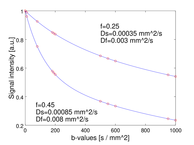
The most used model separating the contribute of diffusion and perfusion in intra-voxel incoherent motion has been developed by Le Bihan [5]. According to this pioneering paper, the signal intensity of diffusion weighted MRI can be described by eq. 2.1:

			$\displaystyle S(b,S_{0},f,D,D^{*})=$
		$\displaystyle=$	$\displaystyle S_{0}\left[(1-f)\exp(-bD)+f\exp\left(-b(D+D^{*})\right)\right]$

where $b$ is a factor depending on the gradient pulse sequence, $D$ is the diffusion coefficient of water, $D^{*}$ is a pseudo-diffusion coefficient describing blood microcirculation, $f$ is the fraction of water flowing in perfused capillary, $S_{0}$ is the signal intensity when $b=0$ .

As suggested in [4], eq. 2.1 can be rearranged as in eq. 2.1:

			$\displaystyle S(b,S_{0},f,D_{s},D_{f})=$
		$\displaystyle=$	$\displaystyle S_{0}\left[(1-f)\exp(-bD_{s})+f\exp\left(-bD_{f}\right)\right]$

where $D_{s}=D$ represents the slow component of diffusion and $D_{f}=D+D^{*}$ represents the fast component of diffusion. This form slightly simplifies formula manipulation and will be used in the following.

Units of the diffusion coefficients are $\mathrm{mm}^{2}/\mathrm{s}$ while $b$ is measured in $\mathrm{s}/\mathrm{mm}^{2}$ . Typically [5, 4], $D_{f}$ is about $20\cdot 10^{-3}\mathrm{mm}^{2}/\mathrm{s}$ while $D_{s}$ is about $1\cdot 10^{-3}\mathrm{mm}^{2}/\mathrm{s}$ . In general $D_{f}>>Ds$ . Values for $b$ , which is the focus of this paper, falls typically in the range $0\rightarrow 1000\quad\mathrm{s}/\mathrm{mm}^{2}$ . Perfusion fraction $f$ has no units and ranges $0<f<1$ .

2.2 Noise on diffusion weighted data

It is well known that, because of noise superimposed to receiving antennas, the measured signal intensity ( $S_{m}$ ) of diffusion MRI data has a Rician distribution [8] as in eq. 3:

p(S_{m};S,\sigma)=\frac{S_{m}}{\sigma^{2}}\exp\left(-\frac{S_{m}^{2}+S^{2}}{2\sigma^{2}}\right)I_{0}\left(\frac{S_{m}S}{\sigma^{2}}\right)

(3)

where $S$ is the signal intensity without noise (which should be given by the IVIM model eq. 2.1), $\sigma$ is the noise level, $I_{0}$ is the modified Bessel function of the first kind.

It the limit of high Signal Noise Ratio (SNR, $S/\sigma>3$ ) the distribution can be well approximated by a Gaussian distribution [8, 9]:

p(S_{m};S,\sigma)\approx\frac{1}{\sqrt{2\pi\sigma^{2}}}\exp\left(-\frac{(S_{m}-\sqrt{S^{2}+\sigma^{2}})^{2}}{2\sigma^{2}}\right)

(4)

In our experience, on diffusion images of the prostate at several $b$ -values from 0 to 1000, the approximation $S>>\sigma$ is very well satisfied. In fact, for voxels within region of interest (ROI) the measured intensity $S_{m}(b)$ is about $100$ for $b=0$ decreasing to about $50$ when $b=1000\quad\mathrm{s}/\mathrm{mm}^{2}$ ; the $\sigma$ parameter evaluated outside the field of view, gives a value of about $2$ ( $S/\sigma\approx 50$ ). At our institution images have been obtained using a Siemens scanner, 1.5 T, with pulse sequences EP (SK/SP/OSP), TR = 7500 ms, TE = 91 ms, 3 averages, flip angle = 90 deg.

Moreover, the SNR measures reported in [4] confirm that the noise level $\sigma$ is typically very low with respect to the signal level $S$ .

Generalising the previous considerations, in the following we will assume that the hypothesis of Gaussian approximation is satisfied; additionally, we will assume that to a very good approximation $\sqrt{S^{2}+\sigma^{2}}\approx S$ as $S>>\sigma$ , and therefore the measured signal is:

S_{m}=S+\epsilon

(5)

with additive noise $\epsilon\sim\mathcal{N}(0,\sigma)$ .

2.3 IVIM model for $b$ optimisation

It is a common approach in IVIM literature to normalise DW data $S_{m}(b)$ dividing by $S_{m}(0)$ because in so doing the model simplifies to a three parameters model. Typically, a Least Squares (LS) fitting is applied [10, 5, 4] assuming, implicitly [7], that the noise onto the normalised data $S_{m}(b)/S_{m}(0)$ is additive gaussian.

However, as it has been observed in the previous section, while the noise superimposed on $S$ can be well approximated (for $S/\sigma>3$ ) by a gaussian distribution, the distribution of $S_{m}(b)/S_{m}(0)$ becomes a Cauchy distribution instead [11]. As a consequence, the LS approach to non linear fitting, which is derived within the framework of Maximum Likelihood under the hypothesis of spherical Gaussian distribution, might be not adequate in this case.

With this in mind, for $b$ design purposes (section 2.4) and for evaluation of attainable accuracy (section 2.5) we consider here a complete 4 parameters model $S(b,S_{0},f,D_{s},D_{f})$ including $S_{0}$ among the parameters, instead of the common approach to consider the normalised signal.

2.4 D-optimal design

As underlined in the previous section, DW signal intensities in real cases can be be typically well approximated by a Gaussian distribution, implying that the measured signal $S_{m}(b)$ has an IVIM component plus an additive noise component as in eq. (6):

S_{m}(b;S_{0},\boldsymbol{\theta})=S(b,S_{0},\boldsymbol{\theta})+\epsilon

(6)

with $\epsilon$ having Gaussian distribution $\mathcal{N}(0,\sigma)$ with zero mean and standard deviation $\sigma$ , and $\boldsymbol{\theta}=[f,D_{s},D_{f}]^{T}$ .

Under this hypothesis it is possible to use the theory for optimal design of experiments described, for example, in [7, 6]. Optimal design is based upon the computation of the Fisher information matrix of the IVIM model, which we perform in the following.

The Fisher information matrix corresponding to all parameters $\mathbf{p}=[S_{0},f,D_{s},D_{f}]^{T}$ is given by eq 7:

	$\displaystyle\mathbf{M}$	$\displaystyle=$	$\displaystyle\{M_{ij}\}=\sigma^{-2}\sum_{k=1}^{N}\frac{\partial S(b_{k})}{\partial p_{i}}\frac{\partial S(b_{k})}{\partial p_{j}}=$		(7)
		$\displaystyle=$	$\displaystyle\sigma^{-2}\frac{\partial S(\mathbf{b}^{T})}{\partial\mathbf{p}}\frac{\partial S(\mathbf{b})}{\partial\mathbf{p}^{T}}$		(7)

where the partial derivatives of $S$ are evaluated at $b_{k}$ with $\mathbf{b}=[b_{1},b_{2},\ldots,b_{N}]^{T}$ . However, we note that the model in eq. (2.1) is conditionally linear in the parameter $S_{0}$ , thus it can be re-formulated as:

S(b;S_{0},\boldsymbol{\theta})=S_{0}\cdot g(b,\boldsymbol{\theta})

(8)

where

g(b,\boldsymbol{\theta})=(1-f)\exp(-bD_{s})+f\exp\left(-bD_{f}\right)

(9)

and therefore the Fisher Matrix can be rewritten as:

	$\displaystyle\mathbf{M}$	$\displaystyle=$	$\displaystyle\sigma^{-2}\left(\begin{array}[]{cc}1&\mathbf{0}\\ \mathbf{0}&S_{0}\mathbf{I}\\ \end{array}\right)\mathbf{J}^{T}\mathbf{J}\left(\begin{array}[]{cc}1&\mathbf{0}\\ \mathbf{0}&S_{0}\mathbf{I}\\ \end{array}\right)$
		$\displaystyle=$	$\displaystyle\sigma^{-2}\mathbf{A}^{T}(S_{0})\mathbf{J}^{T}\mathbf{JA}(S_{0})$

where $\mathbf{I}$ is the identity matrix of size $3\times 3$ , $\mathbf{A}(S_{0})$ depends only on $S_{0}$ and

	$\displaystyle\mathbf{J}(\mathbf{b},\boldsymbol{\theta})$	$\displaystyle=$	$\displaystyle\left(\begin{matrix}g(b_{1},\boldsymbol{\theta})&\frac{\partial g(b_{1},\boldsymbol{\theta})}{\partial f}&\frac{\partial g(b_{1},\boldsymbol{\theta})}{\partial D_{s}}&\frac{\partial g(b_{1},\boldsymbol{\theta})}{\partial D_{f}}\\ g(b_{2},\boldsymbol{\theta})&\frac{\partial g(b_{2},\boldsymbol{\theta})}{\partial f}&\frac{\partial g(b_{2},\boldsymbol{\theta})}{\partial D_{s}}&\frac{\partial g(b_{2},\boldsymbol{\theta})}{\partial D_{f}}\\ \vdots&\vdots&\vdots&\vdots\\ g(b_{N},\boldsymbol{\theta})&\frac{\partial g(b_{N},\boldsymbol{\theta})}{\partial f}&\frac{\partial g(b_{N},\boldsymbol{\theta})}{\partial D_{s}}&\frac{\partial g(b_{N},\boldsymbol{\theta})}{\partial D_{f}}\end{matrix}\right)$		(15)
		$\displaystyle=$	$\displaystyle[\mathbf{g},~\partial_{f}\mathbf{g},~\partial_{D_{s}}\mathbf{g},~\partial_{D_{f}}\mathbf{g}]$		(15)

where the four columns of $\mathbf{J}$ have been indicated by vectors for simplicity.

Further simplification can be obtained using the following notation:

	$\displaystyle\mathbf{E}_{s}$	$\displaystyle=$	$\displaystyle\exp(-\mathbf{b}D_{s})$
	$\displaystyle\mathbf{E}_{f}$	$\displaystyle=$	$\displaystyle\exp(-\mathbf{b}D_{f})$		(16)

which gives $\mathbf{g}=(1-f)\mathbf{E}_{s}+f\mathbf{E}_{f}$ and $\partial_{f}\mathbf{g}=\mathbf{E}_{f}-\mathbf{E}_{s}$ . Moreover, we indicate with $\circ$ the Hadamard product between two vectors e.g.:

\mathbf{x}\circ\mathbf{y}=[x_{1}y_{1},\ldots,x_{N}y_{N}]^{T};

(17)

which gives $\partial_{D_{s}}\mathbf{g}=-(1-f)\mathbf{b}\circ\mathbf{E}_{s}$ and $\partial_{D_{f}}\mathbf{g}=-f\mathbf{b}\circ\mathbf{E}_{f}$ .

With this notations the matrix $\mathbf{J}$ can be rewritten:

	$\displaystyle\mathbf{J}(\mathbf{b},\boldsymbol{\theta})=$	(18)
$\displaystyle=$	$\displaystyle[\mathbf{E}_{s},\mathbf{E}_{f},\mathbf{b}\circ\mathbf{E}_{s},\mathbf{b}\circ\mathbf{E}_{f}]\left(\scalebox{0.75}{\mbox{$\displaystyle\begin{matrix}1-f&-1&0&0\\ f&1&0&0\\ 0&0&-(1-f)&0\\ 0&0&0&-f\end{matrix}$}}\right)$
$\displaystyle=$	$\displaystyle\mathbf{H}(\mathbf{b},D_{s},D_{f})\mathbf{B}(f)$

According to the D-optimal design approach we must find the $b$ values maximizing the determinant ( $||\cdot||$ ) of the Fisher matrix:

			$\displaystyle\|\|\mathbf{M}(\mathbf{b},S_{0},\boldsymbol{\theta})\|\|=$		(19)
		$\displaystyle=$	$\displaystyle\sigma^{-2}\|\|\mathbf{A}(S_{0})\|\|^{2}\|\|\mathbf{B}(f)\|\|^{2}\|\|\mathbf{H}^{T}\mathbf{H}(\mathbf{b},D_{s},D_{f})\|\|$		(19)

it is clear that the optimal value for $\mathbf{b}$ can be found independently from $S_{0}$ and $f$ :

\mathbf{b}_{opt}=\arg\max_{\mathbf{b}\in\mathcal{B}}\left(\min_{D_{s},D_{f}\in\boldsymbol{\Theta}}\left\lVert\mathbf{H}^{T}\mathbf{H}\right\rVert\right)

(20)

where $\mathcal{B}$ is the design space (the set of all candidate $b$ -values) and $\boldsymbol{\Theta}$ a region of interest within the parameters space (containing the expected values of the parameters).

It is well known [6] that the number of $b$ -values (design points) must be grater (or equal) than the total number of parameters $P$ (4 in this case) in order for $\mathbf{M}$ not to be singular. Moreover, in a continuous design [6] (i.e. when the number of measurements taken at the design points is very large) the number of design points is limited superiorly by $P(P+1)/2+1$ (11 in the present case). In passing to a discrete design (i.e. a single measure is taken at each design point, as is the case for IVIM studies) the number could be greater than this limit. However, we used 20 as maximum because of the previous considerations (see Introduction section) concerning the duration of the exam

2.5 Comparison of designs

To compare different designs we used the Cramer-Rao lower bound (CRLB) [12, 13, 6, 7] Assuming the parameters estimates are not biased, according to the Cramer-Rao lower bound theorem [13] the achievable accuracy is given by the diagonal elements of the inverse Fisher information matrix. The inverse of the Fisher matrix is given by:

\mathbf{M}^{-1}=\sigma^{2}\left(\begin{array}[]{cc}1&\mathbf{0}\\ \mathbf{0}&S_{0}^{-1}\mathbf{I}\\ \end{array}\right)(\mathbf{J}^{T}\mathbf{J})^{-1}\left(\begin{array}[]{cc}1&\mathbf{0}\\ \mathbf{0}&S_{0}^{-1}\mathbf{I}\\ \end{array}\right)

(21)

Calling $j^{-1}_{kk}$ with $k=1,\ldots,4$ , the diagonal elements of the matrix $(\mathbf{J}^{T}\mathbf{J})^{-1}$ we have the following bounds for the estimated parameters:

\left(\begin{array}[]{ccc}\sigma_{f}^{2}&&\\ &\sigma_{D_{s}}^{2}&\\ &&\sigma_{D_{f}}^{2}\end{array}\right)\succeq\frac{\sigma^{2}}{S_{0}^{2}}\left(\begin{array}[]{ccc}j^{-1}_{22}&&\\ &j^{-1}_{33}&\\ &&j^{-1}_{44}\end{array}\right)

(22)

and $\sigma^{2}j^{-1}_{11}$ is the CRLB of the variance of $S_{0}$ estimator, which is of no interest here. The square root of CRLB ( $\sigma_{f}$ , $\sigma_{D_{s}}$ , $\sigma_{D_{f}}$ ) can be considered the achievable accuracy for the parameter estimate.

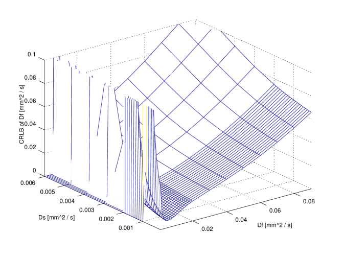
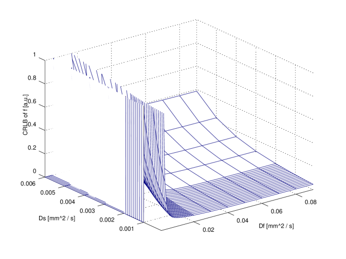
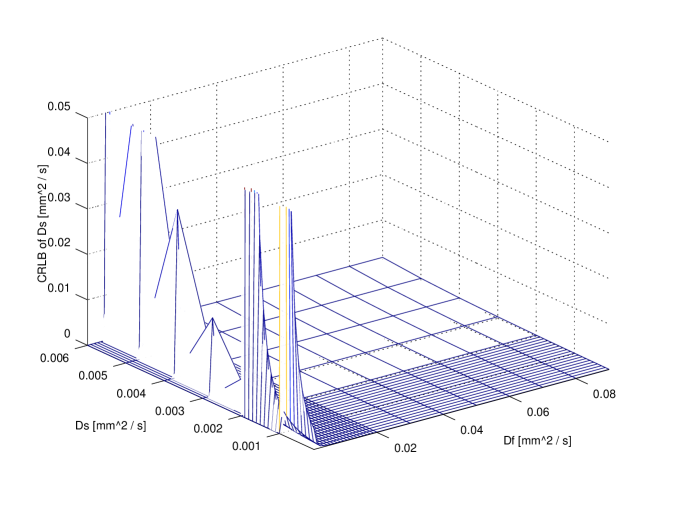
We have computed the square root of CRLB per each parameter at the $\mathbf{b}_{opt}$ D-optimal values (eq. 20), over the whole parameters region used in the optimisation process.

2.6 Numerical optimisation

2.6.1 Parameters region

The region of the parameter space $\boldsymbol{\Theta}$ has been chosen on the basis of parameters values found in published literature: see table 1.

Table 1: Values of IVIM parameters used in previous simulation studies. The notation used is Octave-like: the number between two colons (:) is the increment between the minimum and the maximum of the range.

Study	$D_{s}\cdot 10^{-3}[\mathrm{mm^{2}/s}]$	$D_{f}\cdot 10^{-3}[\mathrm{mm^{2}/s}]$
[4]	0.23, 0.7	2.52, 2.9
[2]	1, 0.5:6	2.1, 15.5:81
[3]	1, 1.5	11, 16.5, 61
this	0.1:0.1:2, 2:1:6	1:1:20, 20:10:90

2.6.2 Range of candidate $b$ values

Also the range of $b$ values has been chosen after examination of literature [1, 3]. In particular, we have used the following set of $b$ -values given as in a Octave-like notation $b$ = 0:10:200, 250:50:1000, (37 values).

2.6.3 Exact design

In principle, according to the max-min criterion (eq. 20), in order to find the optimal $\mathbf{b}$ , it is required to test all the combinations of $b$ -values taken from the series of candidate $b$ -values. Per each combination of $b$ -values, the determinant of eq. 20 must be evaluated on a grid comprising all interesting values $(D_{s},D_{f})$ within the parameter space $\boldsymbol{\Theta}$ and the minimum value over this region has to be found. Afterwards, the $\mathbf{b}$ giving maximum of all minima must be found. This guarantees that the Fisher determinant evaluated at $\mathbf{b}_{opt}$ is the highest possible over the entire parameters region.

However, this approach implies large computational times for designs with a number of design points greater than the minimum (i.e. 4, see section 2.4): this makes also impractical the design based over a large region of the parameters space or the use of an large candidate set of $b$ -values. For these reasons, in the next section we propose to use a fast but approximate design.

2.6.4 Approximate design

As observed the minimum number of design points which gives non singular Fisher matrix for the IVIM model is 4. As a starting point, we found the exact optimal 4 points design using the method described in the previous section : $\mathbf{b}_{opt}(4)=[0,80,500,1000]$ . In particular, we evaluated the determinant of the Fisher matrix over all the parameters space $\boldsymbol{\Theta}$ and using as $\mathcal{B}$ the space of all possible combinations of 4 points chosen among the 37 candidate $b$ values chosen. The resulting number of combinations in this case is $\scalebox{0.75}{\mbox{$\displaystyle\left(\begin{array}[]{c}{37}\\ {4}\end{array}\right)$}}=66045$ .

However, as observed, with increasing number of design points, the number of possible combination increases quickly (e.g. $\scalebox{0.75}{\mbox{$\displaystyle\left(\begin{array}[]{c}{37}\\ {5}\end{array}\right)$}}=435897$ ), and the computational time increases as well. In order to limit the computational time we proceeded as follows.

Let $\mathbf{b}(N)=[b_{1},\ldots,b_{N}]$ a design set with $N$ points. Starting from an optimal design $\mathbf{b}(N)$ we can construct a new design $\mathbf{b}(N+1)=[\mathbf{b}(N),~b_{new}]$ adding a new $b_{new}$ value. The matrix $\mathbf{H}$ corresponding to this new set of design points is (dropping down the dependence on $D_{s}$ and $D_{f}$ for simplicity):

\mathbf{H}^{T}(\mathbf{b}(N+1))=[\mathbf{H}^{T}(\mathbf{b}(N)),~\mathbf{r}(b_{new})]

(23)

where

\mathbf{r}(b_{new})=\left(\begin{array}[]{c}\exp(-b_{new}D_{s})\\ \exp(-b_{new}D_{f})\\ b_{new}\exp(-b_{new}D_{s})\\ b_{new}\exp(-b_{new}D_{f})\end{array}\right)

(24)

As we are interested in calculation of the determinant of the Fisher matrix we observe that [6] (we drop the dependence from $b_{new}$ , $D_{s}$ and $D_{f}$ in order to simplify notation) :

	$\displaystyle\|\|\mathbf{M}(\mathbf{b}(N+1))\|\|=$		(25)
	$\displaystyle=\|\|\mathbf{M}(\mathbf{b}(N))\|\|\cdot(1+\mathbf{r}^{T}(\mathbf{H}^{T}(N)\mathbf{H}(N))^{-1}\mathbf{r})$

In order for the new design being optimal this determinant must be maximum. This implies that $b_{new}$ must maximise equation 25 over the parameters region. Using equation 25 and starting from the optimal design $\mathbf{b}(4)$ , designs with a fixed $N$ can be constructed iteratively, evaluating one only matrix inverse and performing $\sim N$ computations instead of examining all the possible combinations.

Unfortunately, this algorithm does not provide an absolutely optimal design, because there can be different combinations of $N+1$ points extracted from the original set, giving a higher determinant. This algorithm provides therefore a sub-optimal solution. However, in our experience (we tested the case $N=5$ and $N=6$ ), the accuracy attainable with the sub-optimal solution is not far away from the optimal solution (see figure 3).

3 Results

All optimisations have been performed in Octave [octave].

Table 2 reports the exact designs obtained for $N=4,5,6$ respectively. They have been obtained considering all the possible combinations of $N$ $b$ -values chosen from the candidate set.

Table 3 reports the approximate designs obtained using the algorithm described in section 2.6.4. The first four entries of the table coincide with the 4 points design; starting from this one should add the successive entries in order to obtain designs with more than 4 points. For example a 6 points design includes $0,80,500,1000,190,600$ .

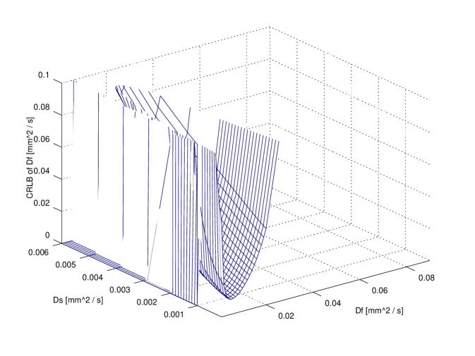
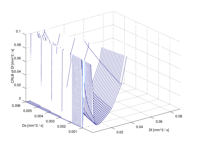
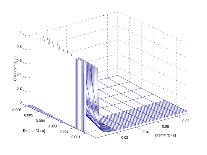
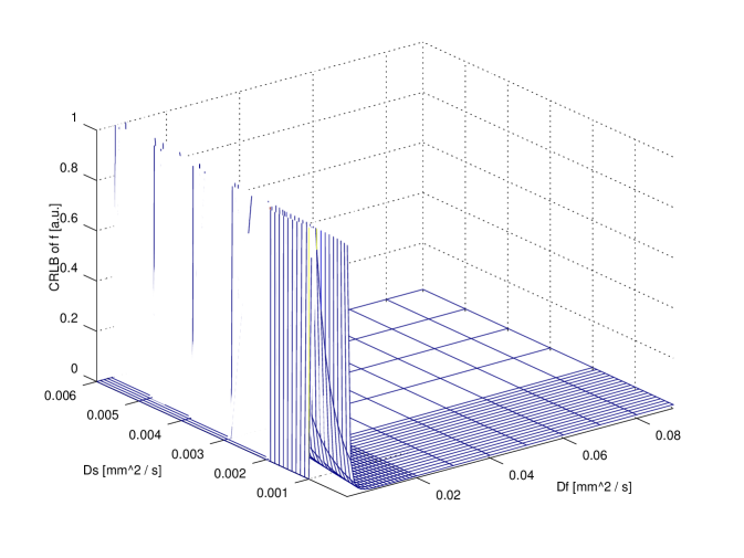
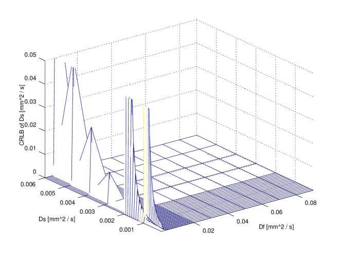
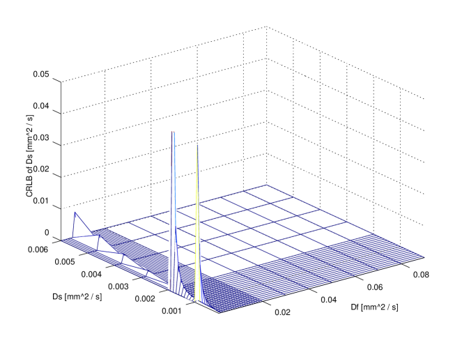
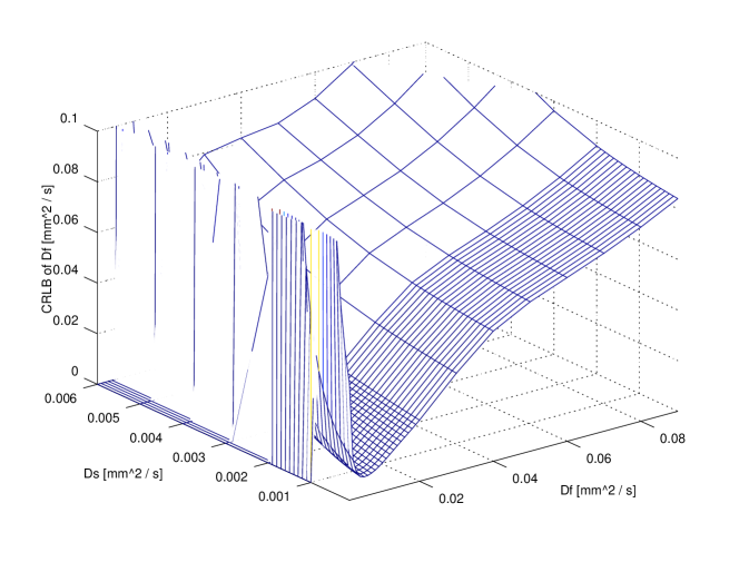
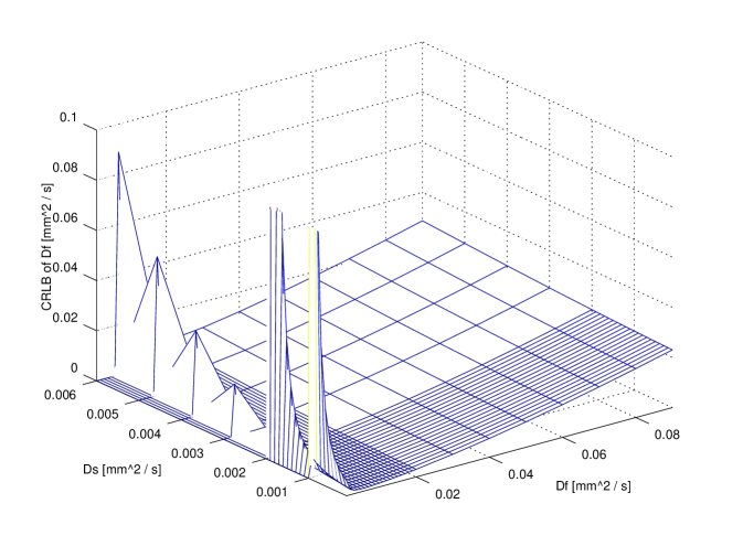
In order to compare exact designs with approximate ones the CRLB can be used: in particular, for illustrative purposes, the comparison between the exact 6 points design and the approximate one is reported in figure 3. The attainable accuracy (CRLB) has been computed over the whole parameter region. It is clear that per each parameter the CRLB with exact design is not very different from the corresponding accuracy attainable using the approximate design.

It is useful to compare the accuracy attainable with design using a small number of points (e.g. 11) with respect to the higher accuracy attainable using a very large $N=1000$ design (e.g. $b=0:1:1000$ , ideal design). The comparison is reported in figure 4. It is evident that no large difference is revealed for $f$ and $D_{s}$ ; on the contrary, ‘ideal’ design gains a significant improvements with respect to the 11 points design: however, in a clinical scenario this might not justify the extra time required. Further insight on this issue can be achieved observing fig 2. As a matter of fact, the use of 20 points does not improve with respect to 11 points design.

In figures 3 and 4 a value of $f=0.1$ has been used; other parameters were $S_{0}=100$ and $\sigma=3$ corresponding to an SNR of $S_{0}/\sigma\approx 3.33$ . These values can be considered to be representative of real values from published literature.

In order to give an idea of the location of the design points, figure 1 shows an example of DW data vs $b$ for two sets of parameters with the 11 design points superimposed.

Table 2: Optimal designs calculated using the exact algorithm described in section 2.4. Per each number of design points (

N

) the combination of

b

-values chosen from the candidate set is reported.

$N$	Exact Design
4	0	80	500	1000
5	0	120	200	550	1000
6	0	120	200	550	600	1000

Table 3: Approximate optimal design. Starting from the exact 4 points design (the first 4 entries in the table) we derived additional

b

-values iteratively using the algorithm proposed in section 2.4. We report results up to

N=20

b

-values.

0	80	500	1000	190	600	950
10	180	550	200	900	20	650
170	450	160	30	850	400

Refer to caption — Figure 1: Example of normalised ( $S(b)/S_{0}$ ) IVIM curve with various parameters. The solid line represents the theoretical curve; circles indicate the $b$ -values sampled using the results of the present study.

4 Discussion

The aim of this paper was to design the $b$ -values for diffusion weighted MRI in an optimal manner suitable for accurate estimation of intra-voxel incoherent motion parameters according to the model in eq. 2.1.

The design has been conducted according to the principles of the D-optimal approach. Optimal combination of $b$ -values has been chosen within a set of predefined values taken from the literature. As the design is affected from the parameters $D_{s},D_{f}$ an exhaustive optimisation within a predefined parameter region has been made.

Our results are in line with other studies in literature [4, 3], which have been conducted via Monte Carlo simulation. Two main disadvantages of the approach via Monte Carlo simulation are: first, in order to have statistical accuracy a large number of simulation must be performed (typically 1000) and per each simulated noisy curve estimation of parameters must be performed (e.g. via least squares fitting); second, due to computational time only a small portion of the parameters region can be explored in reasonable time. In fact, least squares fitting of noisy simulated curves is time consuming and if $S_{0}$ is neglected it might be not suitable to the noise structure on the data (see section 2.2). Finally, as the parameters values ( $f,D_{s},D_{f}$ ) are not known prior to the MR exam it would be desirable to have a set of $b$ values optimised over a large portion of the parameter space.

The approach followed in this study could overcome the above mentioned disadvantages of the Monte Carlo approach. In particular, we showed (section 2.4) that the search for a D-optimal design can be addressed in the 2D space of the diffusion parameters only $(D_{s},D_{f})$ without considering $S_{0}$ and $f$ : this dramatically reduces the computational load.

Moreover, we propose a fast algorithm for finding an approximate design: on the basis of CRLB analysis we showed that the approximate design is comparable to the exact design (at least in the case of 5 and 6 points designs). In fact, inspection of table 3 and 2 reveals that the approximate designs with 5 and 6 points are only slightly different from the exact 5 and 6 points design. These similarities is confirmed analysing the CRLB in figure 3. From these similarities we infer that also for higher values of $N$ the exact and approximate designs might be very similar (for $N\rightarrow\infty$ the exact and approximate design should converge [6]).

The comparison of 11 points design with the 1000 points design (see figure 4) suggest that even with an ideal design the uncertainty over $D_{f}$ is limited. Furthermore, use of 20 points only slightly improves the accuracy with respect of a 11 points design: this is a useful information in a clinical setting.

A consideration about the hypothesis underlying this study must be made. We used the approximation of Gaussian noise with mean $\approx S$ instead of $\sqrt{S^{2}+\sigma^{2}}$ because our aim was the design of $b$ -values and not the estimation of parameters. As a matter fact, the estimation of parameters is slightly biased and care must be taken in the choice of estimator [9]

One final remark is the following. Our study has shown that it is possible to search for an optimal $N+1$ -point design starting from an (approximately) optimal design of $N$ points. This procedure is very fast. This might suggest an adaptive strategy for D-optimal design which could be performed during clinical exam: after a first scan using the minimum set of 4 $B$ -values, an estimate $\boldsymbol{\theta}_{0}$ of the parameters is performed over the region of interest (within the image), opportunely selected by the radiologist; a spatial average of the first estimate might be used for the design of the 5th point; the procedure can be repeated giving estimates $\boldsymbol{\theta}_{1}$ , $\boldsymbol{\theta}_{2}$ and so on. The radiologist can stop after reaching the desired accuracy in the estimates or after a reasonable time. This adaptive procedure has not been investigated here but will be subject of future studies.

5 Conclusion

The design of the $b$ -values for optimal estimation of IVIM parameters can be addressed using a D-optimal strategy. In this study we have shown that the optimal design does not depend on perfusion fraction $f$ and therefore the search can be performed in a 2-D space $(D_{S},D_{f})$ ; moreover, as an exact exhaustive search is still time consuming, we have proposed an iterative algorithm for searching an approximate design starting from an optimal design formed by 4 points.

Acknowledgment

The authors would like to thank Dr. Augusto Aubry at the Dept. of Electrical Engineering and Information Technologies of University of Naples ‘Federico II’ for fruitful discussions.

References

[1] D.-M. Koh, D. J. Collins, and M. R. Orton, “Intravoxel incoherent motion in body diffusion-weighted mri: reality and challenges,” AJR Am J Roentgenol, vol. 196, no. 6, pp. 1351–61, Jun 2011.
[2] Q. Zhang, Y.-X. Wang, H. T. Ma, and J. Yuan, “Cramer-rao bound for intravoxel incoherent motion diffusion weighted imaging fitting,” in Engineering in Medicine and Biology Society (EMBC), 2013 35th Annual International Conference of the IEEE. IEEE, 2013, pp. 511–514.
[3] A. Lemke, B. Stieltjes, L. R. Schad, and F. B. Laun, “Toward an optimal distribution of b values for intravoxel incoherent motion imaging,” Magnetic resonance imaging, vol. 29, no. 6, pp. 766–776, 2011.
[4] I. Jambor, H. Merisaari, H. J. Aronen, J. Järvinen, J. Saunavaara, T. Kauko, R. Borra, and M. Pesola, “Optimization of b-value distribution for biexponential diffusion-weighted mr imaging of normal prostate,” Journal of Magnetic Resonance Imaging, vol. 39, no. 5, pp. 1213–1222, 2014.
[5] D. Le Bihan, E. Breton, D. Lallemand, M. Aubin, J. Vignaud, and M. Laval-Jeantet, “Separation of diffusion and perfusion in intravoxel incoherent motion mr imaging.” Radiology, vol. 168, no. 2, pp. 497–505, 1988.
[6] V. V. Fedorov, Theory of optimal experiments. Elsevier, 1972.
[7] D. M. Bates and D. G. Watts, Nonlinear regression: iterative estimation and linear approximations. Wiley Online Library, 1988.
[8] H. Gudbjartsson and S. Patz, “The rician distribution of noisy mri data,” Magnetic resonance in medicine, vol. 34, no. 6, pp. 910–914, 1995.
[9] A. Kristoffersen, “Optimal estimation of the diffusion coefficient from non-averaged and averaged noisy magnitude data,” Journal of Magnetic Resonance, vol. 187, no. 2, pp. 293–305, 2007.
[10] R. Fusco, M. Sansone, and A. Petrillo, “The use of the levenberg–marquardt and variable projection curve-fitting algorithm in intravoxel incoherent motion method for dw-mri data analysis,” Applied Magnetic Resonance, vol. 46, no. 5, pp. 551–558, 2015.
[11] A. P. Probability, “Random variables and stochastic processes,” McGrow, Hill Series Elastical Eng, NY, 1984.
[12] M. Sansone, R. Fusco, and A. Petrillo, “A geometrical perspective on the 3tp method in dce-mri,” Biomedical Signal Processing and Control, vol. 16, pp. 32–39, 2015.
[13] S. Smith, “Covariance, subspace, and intrinsic cramer-rao bounds,” Signal Processing, IEEE Transactions on, vol. 53, no. 5, pp. 1610–1630, May 2005.