DARC: Distribution-Aware Re-Coloring Model for Generalizable Nucleus Segmentation
Abstract
Nucleus segmentation is usually the first step in pathological image analysis tasks. Generalizable nucleus segmentation refers to the problem of training a segmentation model that is robust to domain gaps between the source and target domains. The domain gaps are usually believed to be caused by the varied image acquisition conditions, e.g., different scanners, tissues, or staining protocols. In this paper, we argue that domain gaps can also be caused by different foreground (nucleus)-background ratios, as this ratio significantly affects feature statistics that are critical to normalization layers. We propose a Distribution-Aware Re-Coloring (DARC) model that handles the above challenges from two perspectives. First, we introduce a re-coloring method that relieves dramatic image color variations between different domains. Second, we propose a new instance normalization method that is robust to the variation in foreground-background ratios. We evaluate the proposed methods on two HE stained image datasets, named CoNSeP and CPM17, and two IHC stained image datasets, called DeepLIIF and BC-DeepLIIF. Extensive experimental results justify the effectiveness of our proposed DARC model. Codes are available at https://github.com/csccsccsccsc/DARC.
Keywords:
Domain Generalization Nucleus Segmentation Instance Normalization.1 Introduction
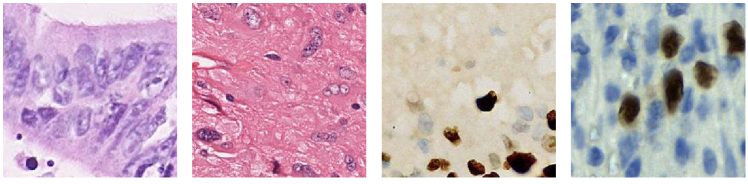
Automatic nucleus segmentation has captured wide research interests in recent years due to its importance in pathological image analysis [1, 2, 3, 4]. However, as shown in Fig. 1, the variations in image modalities, staining protocols, scanner types, and tissues significantly affect the appearance of nucleus images, resulting in notable gap between source and target domains [5, 6, 7]. If a number of target domain samples are available before testing, one can adopt domain adaptation algorithms to transfer the knowledge learned from the source domain to the target domain [8, 9, 10]. Unfortunately, in real-world applications, it is usually expensive and time-consuming to collect new training sets for the ever changing target domains; moreover, extra computational cost is required, which is usually unrealistic for the end users. Therefore, it is highly desirable to train a robust nucleus segmentation model that is generalizable to different domains.
In recent years, the research on domain generalization (DG) has attracted wide attention. Most existing DG works are proposed for classification tasks [12, 13] and they can be roughly grouped into data augmentation-, representation learning-, and optimization-based methods. The first category of methods [14, 15, 16, 17] focus on the way to diversify training data styles and expect the enriched styles cover those appeared in target domains. The second category of methods aim to obtain domain-invariant features. This is usually achieved via improving model architectures [18, 19, 20] or introducing novel regularization terms [21, 22]. The third category of methods [23, 24, 25, 26] develop new model optimization strategies, e.g., meta-learning, that improve model robustness via artificially introducing domain shifts during training.
It is a consensus that a generalizable nucleus segmentation model should be robust to image appearance variation caused by the change in staining protocols, scanner types, and tissues, as illustrated in Fig. 1. In this paper, we argue that it is also desirable to be robust to the ratio between foreground (nucleus) and background pixel numbers. This ratio changes the statistics of each feature map channel, and affects the robustness of normalization layers, e.g., instance normalization (IN). We will empirically justify its impact in Section 2.3.
2 Method
2.1 Overview
In this paper, we adopt a U-Net-based model similar to that in [1] as the baseline. It performs both semantic segmentation and contour detection for nucleus instances. The area of each nucleus instance is obtained via subtraction between the segmentation and contour prediction maps [1]. Details of the baseline model is provided in the supplementary material. To handle domain variations, we adopt IN rather than batch normalization (BN) in the U-Net model.
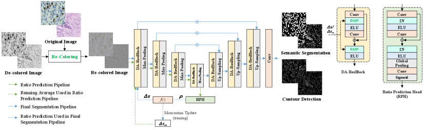
Our proposed Distribution-Aware Re-Coloring model (DARC) is illustrated in Fig. 2. Compared with the baseline, DARC replaces the IN layers with the proposed Distribution-Aware Instance Normalization (DAIN) layers. DARC first re-colors each image to relieve the influence caused by image acquisition conditions. The re-colored image is then fed into the U-Net encoder and the ratio prediction head. This head predicts the ratio between foreground and background pixel numbers. With the predicted ratio, the DAIN layers can estimate feature statistics more robustly and facilitate more accurate nucleus segmentation.
2.2 Nucleus Image Re-Coloring
We propose the Re-Coloring (RC) method to overcome the color change in different domains. Specifically, given a RGB image , e.g., an HE or IHC stained image, we first obtain its grayscale image . We then feed into a simple module that consists of a single residual block and a convolutional layer with output channel number of 3. In this way, we obtain an initial re-colored image .
However, de-colorization results in the loss of fine-grained textures and may harm the segmentation accuracy. To handle this problem, we compensate with the original semantic information contained in . Recent works [40] show that semantic information can be reflected via the order of pixels according to their gray value. Therefore, we adopt the Sort-Matching algorithm [41] to combine the semantic information in with the color values in . Details of RC is presented in Alg. 1, in which and denote channel-wisely sorting the values and obtaining the sorted values and indices respectively, and denotes re-assembling the sorted values according to the provided indices. Details of the module are included in the supplementary material.
| 1 | 2 | 4 | 6 | |
| AJI | 65.11 | 59.11 | 53.41 | 54.13 |
| Dice | 86.14 | 84.05 | 80.97 | 79.75 |
Via RC, the original fine-grained structure information from is recovered in . In this way, the re-colored image is advantageous in two aspects. First, the appearance difference between pathological images caused by the change in scanners and staining protocols is eliminated. Second, the re-colored image preserves fine-grained structure information, enabling precise instance segmentation to be possible.
2.3 Distribution-Aware Instance Normalization
Due to dramatic domain gaps, feature statistics may differ significantly between domains [7, 5, 6], which means that feature statistics obtained from the source domain may not apply to the target domain. Therefore, existing DG works usually replace BN with IN for feature normalization [19, 12]. However, for dense-prediction tasks like semantic segmentation or contour detection, adopting IN alone cannot fully address the feature statistics variation problem. This is because feature statistics are also relevant to the ratio between foreground and background pixel numbers. Specifically, an image with more nucleus instances produces more responses in feature maps and thus higher feature statistic values, and vice versa. The difference in this ratio causes interference to nucleus segmentation.
To verify the above viewpoint, we evaluate the baseline model under different foreground-background ratios. Specifically, we first remove the foreground pixels via in-painting [27], and then pad the original testing images with the obtained background patches. We adopt to denote the ratio between the size of the obtained new image and the original image size. Compared with the original images, the new images have the same foreground regions but more background pixels, and thus have different foreground-background ratios. Finally, we evaluate the performance of the baseline model with different values. Experimental results are presented in Table 1. It is shown that the value of affects the model performance significantly.
The above problem is common in nucleus segmentation because pathological images from different organs or tissues tend to have significantly different foreground-background ratios. However, this phenomenon is often ignored in existing research. To handle this problem, we propose the Distribution-Aware Instance Normalization (DAIN) method to re-estimate feature statistics that account for different ratios of foreground and background pixels. Details of DAIN is presented in Alg. 2. The structures of and are included in the supplemental materials.
As shown in Fig. 2, to obtain the foreground-background ratio of one input image, we first feed it to the model encoder with as the additional input. acts as pseudo residuals of feature statistics and is obtained in the training stage via averaging in a momentum fashion. The output features by the encoder are used to predict the foreground-background ratio with a Ratio-Prediction Head (RPH). is then utilized to estimate the residuals of feature statistics: . Here, is a convolutional layer that transforms to a feature vector whose dimension is the same as the target layer’s channel number. After that, the input image is fed into the model again with as additional input and finally makes more accurate predictions.
The training of RPH requires an extra loss term , which is formulated as bellow:
| (1) |
where denotes the ground truth foreground-background ratio, and and denote the binary cross entropy loss and the mean squared error, respectively.
3 Experiments
3.1 Datasets
The proposed method is evaluated on four datasets, including two HE stained image datasets CoNSeP [3] and CPM17 [28] and two IHC stained datasets DeepLIIF [29] and BC-DeepLIIF [29, 32]. CoNSeP [3] contains 28 training and 14 validation images, whose sizes are pixels. The images are extracted from 16 colorectal adenocarcinoma WSIs, each of which belongs to an individual patient, and scanned with an Omnyx VL120 scanner within the department of pathology at University Hospitals Coventry and Warwickshire, UK. CPM17 [28] contains 32 training and 32 validation images, whose sizes are pixels. The images are selected from a set of Glioblastoma Multiforme, Lower Grade Glioma, Head and Neck Squamous Cell Carcinoma, and non-small cell lung cancer whole slide tissue images. DeepLIIF [29] contains 575 training and 91 validation images, whose sizes are pixels. The images are extracted from the slides of lung and bladder tissues. BC-DeepLIIF [29, 32] contains 385 training and 66 validation Ki67 stained images of breast carcinoma, whose sizes are pixels.
3.2 Implementation Details
In the training stage, patches of size pixels are randomly cropped from the original samples. During training, the batch size is 4 and the total number of training iterations is 40,000. We use Adam algorithm for optimization, and the learning rate is initialized as , which is gradually decreased to during training. We adopt the standard augmentation, like image color jittering and Gaussian blurring. In all experiments, the segmentation and contour detection predictions are penalized using the binary cross entropy loss.
| Methods | CoNSeP | CPM17 | DeepLIIF | BC-DeepLIIF | Average | |||||
| AJI | Dice | AJI | Dice | AJI | Dice | AJI | Dice | AJI | Dice | |
| Baseline (BN) | 16.67 | 24.10 | 33.30 | 61.18 | 08.42 | 38.17 | 21.27 | 39.92 | 19.92 | 40.84 |
| Baseline (IN) | 32.13 | 48.67 | 33.94 | 65.83 | 41.48 | 67.17 | 21.52 | 37.49 | 32.27 | 54.79 |
| BIN [19] | 21.54 | 34.33 | 37.06 | 67.63 | 23.51 | 49.49 | 26.15 | 44.42 | 27.01 | 48.97 |
| DSU [20] | 21.42 | 34.66 | 39.12 | 66.55 | 27.21 | 55.10 | 25.09 | 41.83 | 28.21 | 49.53 |
| SAN [35] | 27.91 | 46.72 | 33.69 | 65.66 | 27.57 | 53.09 | 22.17 | 38.38 | 27.84 | 50.96 |
| AmpNorm [36, 37] | 35.52 | 55.89 | 33.39 | 58.69 | 39.91 | 66.58 | 23.79 | 37.81 | 33.15 | 54.74 |
| StainNorm [38] | 41.06 | 60.81 | 32.75 | 64.68 | 38.55 | 63.95 | 25.41 | 43.81 | 34.44 | 58.11 |
| StainMix [39] | 34.22 | 51.07 | 35.05 | 65.49 | 38.48 | 64.92 | 26.88 | 45.62 | 33.66 | 56.78 |
| TENT (BN) [34] | 38.61 | 58.11 | 35.04 | 64.62 | 33.77 | 59.76 | 23.55 | 40.91 | 32.74 | 55.85 |
| TENT (IN) [34] | 32.34 | 48.87 | 33.24 | 65.73 | 42.08 | 66.87 | 22.38 | 38.04 | 32.51 | 54.88 |
| EFDMix [40] | 40.13 | 58.74 | 33.29 | 65.25 | 39.06 | 64.60 | 25.92 | 42.38 | 34.60 | 57.74 |
| RC (IN)* | 37.21 | 57.53 | 36.98 | 67.71 | 35.53 | 62.03 | 24.98 | 42.25 | 33.68 | 57.38 |
| DAIN* | 33.86 | 50.08 | 30.62 | 64.64 | 37.93 | 65.56 | 31.20 | 53.15 | 33.40 | 58.87 |
| DAIN w/o Ratio* | 27.37 | 40.35 | 33.25 | 65.05 | 40.21 | 66.82 | 29.16 | 48.30 | 32.50 | 55.13 |
| DARCall* | 38.18 | 57.27 | 34.44 | 66.11 | 39.10 | 67.07 | 31.64 | 53.81 | 35.84 | 61.06 |
| DARCenc* | 40.04 | 58.73 | 35.60 | 66.50 | 40.11 | 68.23 | 32.56 | 53.86 | 37.08 | 61.83 |
| Models | Parameters (M) | Inference Time (s/image) |
| Baseline (IN) | 5.03 | 0.0164 |
| DARCenc | 5.47 | 0.0253 |
3.3 Experimental Results and Analyses
In this paper, the models are compared using the AJI [33] and Dice scores. In the experiments, models trained on one of the datasets will be evaluated on the three unseen ones. To avoid the influence of the different sample numbers of the datasets, we calculate the average scores within each unseen domain respectively and then average them across domains.
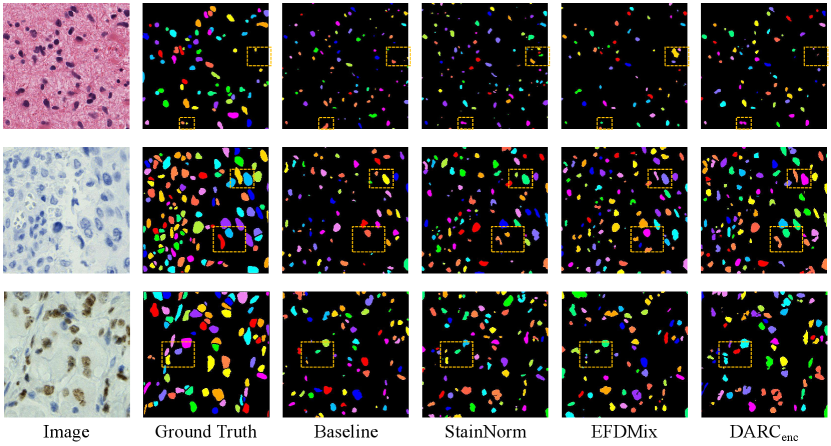
In this paper, we re-implement some existing popular domain generalization algorithms for comparisons under the same training conditions. Specifically, we re-implement the TENT [34], BIN [19], DSU [20], Frequency Amplitude Normalization (AmpNorm) [36, 37], SAN [35] and EFDMix [40]. We also evaluate the stain normalization [38] and stain mix-up [39] methods that are popular in pathological image analysis. Their performances are presented in Table 2. DARCall replaces all normalization layers with DAIN, while DARCenc replaces the normalization layers in the encoder with DAIN and uses BN in its decoder. As shown in Table 2, DARCenc achieves the best average performance among all methods. Specifically, DARCenc improves the baseline model’s average AJI and Dice scores by and . Compared with the other domain generalization methods, DAIN, DAIN w/o Ratio, DARCall and DARCenc achieve impressive performances on BC-DeepLIIF, which justify that re-estimating the instance-wise statistics is important for improving the domain generalization ability of models trained on BC-DeepLIIF. Qualitative comparisons are presented in Fig. 3. Moreover, the complexity analysis between the baseline model and DARCenc is presented in Table 3.
We separately evaluate the effectiveness of RC and DAIN, and present the results in Table 2. Also, we train a variant model without foreground-background ratio prediction, which is denoted as ‘DAIN w/o Ratio’ in Table 2. Compared with the baseline model, RC improves the average AJI and Dice scores by 1.41 and 2.59, and DAIN improves the average AJI and Dice scores by 1.13 and 4.08. Compared with the variant model without foreground-background ratio prediction, DAIN improves the average AJI and Dice scores by 0.90 and 3.74. Finally, the combinations of RC and DAIN, i.e., DARCall and DARCenc, achieve the best average scores. As shown in Table 2, DARCenc improves DARCall by 1.24 and 0.77 on AJI and Dice scores respectively. This is because after the operations by RC and DAIN in the encoder, the obtained feature maps are much more robust to the domain gaps, which enables the decoder to adopt the fixed statistics maintained during training. Moreover, using the fixed statistics is helpful to prevent the decoder from the influence of varied foreground-background ratios on feature statistics.
4 Conclusion
In this paper, we propose the DARC model for generalizable nucleus segmentation. To handle the domain gaps caused by varied image acquisition conditions, DARC first re-colors the input image while preserving its fine-grained structures as much as possible. Moreover, we find that the performance of instance normalization is sensitive to the varied ratios in foreground and background pixel numbers. This problem is well addressed by our proposed DAIN. Compared with existing works, DARC achieves significantly better performance on average across four benchmarks.
References
- [1] Chen, H., Qi, X., Yu, L., Dou, Qi, Qin, J., and Heng, P.-A.: DCAN: Deep contour-aware networks for object instance segmentation from histology images. In: Medical Image Analysis, 36, pp. 135-146 (2017).
- [2] Zhou, Y., Onder, O. F., Dou, Q., Tsougenis, E., Chen, H., and Heng, P. A.: Cia-net: Robust nuclei instance segmentation with contour-aware information aggregation. In: IPMI, pp. 682-693 (2019).
- [3] Graham, S., Vu, Q. D., Raza, S.E.A., Azam, A., Tsang, Y.W., Kwak, J.T. and Rajpoot, N.: Hover-Net: Simultaneous segmentation and classification of nuclei in multi-tissue histology images. In: Medical Image Analysis, 58, p. 101563 (2019).
- [4] Schmidt, U., Weigert, M., Broaddus, C. and Myers, G.: Cell Detection with Star-Convex Polygons. In: MICCAI, pp. 265–273 (2018).
- [5] BenTaieb, A., and Hamarneh, G. Adversarial stain transfer for histopathology image analysis. In: IEEE Transactions on Medical Imaging, 37(3), pp. 792-802 (2018).
- [6] Stacke, K., Eilertsen, G., Unger, J. and Lundström, C.: Measuring Domain Shift for Deep Learning in Histopathology," In: IEEE Journal of Biomedical and Health Informatics, 25(2), pp. 325-336 (2021).
- [7] Aubreville M., et al.: Mitosis domain generalization in histopathology images — The MIDOG challenge. In: Medical Image Analysis, 84, p. 102699 (2023).
- [8] Li, C., et al.: Domain adaptive nuclei instance segmentation and classification via category-aware feature alignment and pseudo-labelling. In: MICCAI pp. 715-724 (2022).
- [9] Liu, D., et al.: PDAM: A Panoptic-Level Feature Alignment Framework for Unsupervised Domain Adaptive Instance Segmentation in Microscopy Images. In: IEEE Transactions on Medical Imaging, 40(1), pp. 154-165 (2021).
- [10] Yang, S., Zhang, J., Huang, J., Lovell, B. C., and Han, X.: Minimizing Labeling Cost for Nuclei Instance Segmentation and Classification with Cross-domain Images and Weak Labels. In: AAAI, 35(1), pp. 697-705 (2021).
- [11] Gulrajani I., Lopez-Paz D.: In search of lost domain generalization. In: ICLR, (2021).
- [12] Zhou, K., et al.: Domain generalization: A survey. In: IEEE Transactions on Pattern Analysis and Machine Intelligence (2022).
- [13] Wang, J., et al.: Generalizing to unseen domains: A survey on domain generalization. In: IEEE Transactions on Knowledge and Data Engineering (2022).
- [14] Huang, J., et al.: Fsdr: Frequency space domain randomization for domain generalization. In: CVPR, pp. 6891-6902 (2021).
- [15] Yang Shu, Zhangjie Cao, Chenyu Wang, Jianmin Wang, Mingsheng Long Shu, Y., Cao, Z., Wang, C., Wang, J., and Long, M.: Open domain generalization with domain-augmented meta-learning. In: CVPR, pp. 9624-9633 (2021).
- [16] Zhou, Z., Qi, L., Shi, Y.: Generalizable Medical Image Segmentation via Random Amplitude Mixup and Domain-Specific Image Restoration. In: ECCV, pp. 420–436 (2022)
- [17] Liu, Q., Chen, C., Qin, J., Dou, Q., and Heng, P.-A.FedDG: Federated Domain Generalization on Medical Image Segmentation via Episodic Learning in Continuous Frequency Space. In: CVPR, pp. 1013-1023 (2021).
- [18] Jin, X., Lan, C., Zeng, W., Chen, Z., and Zhang L.: Style normalization and restitution for generalizable person re-identification. In: CVPR, pp. 3143-3152 (2020).
- [19] Nam, H. and Kim, H.-E.: Batch-instance Normalization for Adaptively Style-invariant Neural Networks. In NeurIPS, pp. 2563–2572 (2018).
- [20] Li, X., Dai, Y., Ge, Y., Liu, J., Shan, Y. and DUAN, L.: Uncertainty Modeling for Out-of-Distribution Generalization. In ICLR (2022).
- [21] Li, H., Pan, S. J., Wang, S., and Kot, A. C.: Domain generalization with adversarial feature learning. In: CVPR, pp. 5400–5409 (2018).
- [22] Tian, C. X., Li, H., Xie, X., Liu, Y., and Wang S.: Neuron coverage guided domain generalization. In: IEEE Transactions on Pattern Analysis and Machine Intelligence 45(1), pp. 1302-1311 (2023).
- [23] Robey, A., Pappas, G. J., and Hassani, H.: Model-based domain generalization. In: NeurIPS, pp. 20210-20229 (2021).
- [24] Qiao, F., Zhao, L., and Peng, X..: Learning to learn single domain generalization. In: CVPR, pp. 12556-12565 (2020).
- [25] Wang, Z., Luo, Y., Qiu, R., Huang, Z., and Baktashmotlagh M.: Learning to diversify for single domain generalization. In: ICCV, pp. 834-843 (2021).
- [26] Shi, Y., et al.: Gradient matching for domain generalization. In: ICLR (2022).
- [27] Telea, A.: An Image Inpainting Technique Based on the Fast Marching Method. In Journal of Graphics Tools, 9(1), pp. 23-24 (2004).
- [28] Vu, Q.D., et al.: Methods for segmentation and classification of digital microscopy tissue images. In Frontiers in bioengineering and biotechnology, p. 53 (2019).
- [29] Ghahremani, P., Marino, J., Dodds, R., and Nadeem, S.: DeepLIIF: An Online Platform for Quantification of Clinical Pathology Slides. In CVPR, pp. 21399-21405 (2022).
- [30] Ronneberger, O., Fischer, P. and Brox, T.: U-net: Convolutional networks for biomedical image segmentation. In MICCAI, pp. 234-241 (2015).
- [31] Llewellyn, B.D.: Nuclear staining with alum hematoxylin. In Biotechnic & Histochemistry, 84(4), pp.159-177 (2009).
- [32] Huang, Z., et al.: BCData: A Large-Scale Dataset and Benchmark for Cell Detection and Counting. In MICCAI, pp. 289–298 (2020).
- [33] Kumar, N., Verma, R., Sharma, S., Bhargava, S., Vahadane, A. and Sethi, A., 2017. A dataset and a technique for generalizable nuclear segmentation for computational pathology. In IEEE Transactions on Medical Imaging, 36(7), pp.1550-1560 (2017).
- [34] Wang, D., Shelhamer, E., Liu, S., Olshausen, B. and Darrell, T.: Tent: Fully Test-time Adaptation by Entropy Minimization. In ICLR (2021).
- [35] Peng, D., Lei, Y., Hayat, M., Guo, Y. and Li, W.: Semantic-aware domain generalizable segmentation. In CVPR, pp. 2594-2605 (2022).
- [36] Jiang, M., Wang, Z. and Dou, Q.: Harmofl: Harmonizing Local and Global Drifts in Federated Learning on Heterogeneous Medical Images. In AAAI 36(1), pp. 1087-1095 (2022).
- [37] Zhao1, X., Liu, C., Sicilia, A., Hwang, S. J., and Fu, Y.: Test-time Fourier Style Calibration for Domain Generalization. In IJCAI (2022).
- [38] Macenko, M., et al.: A method for normalizing histology slides for quantitative analysis. In ISBI, pp. 1107-1110 (2009).
- [39] Chang, J.-R., et al.: Stain Mix-Up: Unsupervised Domain Generalization for Histopathology Images. In MICCAI, pp. 117-126 (2021).
- [40] Zhang, Y., Li, M., Li, R., Jia, K., and Zhang L.: Exact feature distribution matching for arbitrary style transfer and domain generalization. In: CVPR, pp. 8035-8045 (2022).
- [41] Rolland, J.P., Vo, V., Bloss, B. and Abbey, C.K.: Fast algorithms for histogram matching: Application to texture synthesis. In: Journal of Electronic Imaging, 9(1), pp.39-45 (2000).