Dark matter candidate from torsion
Abstract
The stable pseudo-scalar degree of freedom of the quadratic Poincaré Gauge theory of gravity is shown to be a suitable dark matter candidate. We find the parameter space of the theory which can account for all the predicted cold dark matter, and constrain such parameters with astrophysical observations.
Introduction.— Several cosmological and astrophysical phenomena cannot be explained resorting to General Relativity (GR) and the matter content of the Standard Model of Particles (SM). For instance, the present day accelerated expansion of the Universe [1], and the rotational curves of galaxies do not fit the GR predictions with baryonic matter [2]. These problems are solved assuming GR as the correct gravitational framework and modelling the accelerated expansion with a new form of energy (dark energy) encoded in a cosmological constant [3], and the rotation curves by adding a new form of matter known as cold dark matter (CDM). The mentioned approach suffers from some shortcomings: the theoretical value of exceeds the observational value by 120 orders of magnitude [4], and there is no direct nor conclusive evidence of the CDM particles besides their gravitational effects at astrophysical scales [5].
Another approach is to investigate if both the accelerated expansion and the rotation curves can be understood from modifications of GR. Any Lorentz invariant four-dimensional local modification of the Einstein-Hilbert action of GR necessarily introduces new degrees of freedom (d.o.f.s). Then, we can ask if such d.o.f.s can be used to model dark matter and/or dark energy. This line of thought has been explored in the literature for some modifications of GR (see [6, 7, 8]).
We shall work with the Poincaré Gauge modification of GR. This theory arises naturally when promoting the global Poincaré symmetry to a local one, following the gauge procedure. Then, the torsion tensor , which is the antisymmetric part of the spacetime connection , can be identified as the gauge field strength of spacetime translations . Also, the Riemann tensor is given as the gauge field strength of the homogeneous Lorentz group . As usual in Yang-Mills theories, one can construct the Lagrangian considering up to quadratic terms in the field strengths,
| (1) | |||||
which is known as Poincaré Gauge Gravity (PGG) [9, 10]. We know from [11] that, apart from the usual graviton, the matter content of PGG consists of two massive spin-2, two massive spin-1 and two spin-0 fields. In [12, 13, 14] authors found that the only modes that could propagate safely were the two spin-0 with different parity.
In this letter we study the pseudo-scalar mode and show that it behaves like an axion-like particle (ALP). Then, we find the experimental constraints from the interaction of such a mode with the SM sector. Finally, we give the conditions for which the pseudo-scalar mode of PGG can describe the predicted CDM density.
The pseudo-scalar mode.— By considering , , , and in (1), we get the PGG Lagrangian whose only propagating mode is the pseudo-scalar,
| (2) |
Here is the Holst term [15, 16], the denotes quantities calculated with respect to the Levi-Civita (LC) connection, , , and . Also, and represent the trace vector and axial vector of the torsion tensor respectively.
Introducing an auxiliary field , one rewrites (2) as
| (3) |
The massless theory with and without the potential was first considered in [17]. Independently, such a theory was proposed as an extension of GR inspired by Loop Quantum Gravity [18, 19, 20, 21].
From (3), the effective action of the pseudo-scalar can be constructed. First, we need to take into account the couplings to matter for such a Lagrangian, which in the minimal coupling prescription is just given by the coupling of the axial torsion vector to the axial current of fermions [22]. Secondly, by resorting to the field equations for the trace and axial vectors we can isolate such vectors with respect to the rest of variables. Plugging that back to (3) we find (see [14] for details):
| (4) |
Due to the characteristic derivative coupling to a current, this pseudo-scalar d.o.f. can be identified as an ALP [23].
At tree-level the pseudo-scalar couples to fermionic particles only through a derivative coupling. When considering quantum corrections, new interactions arise due to the so-called axial anomaly [24]. In the case of a curved spacetime, such an anomaly can be expressed as [25]
| (5) |
where is the electron charge, denotes the usual electromagnetic tensor, refers to its dual, and is known as the Chern–Pontryagin scalar.
In order to find the couplings of the pseudo-scalar, we first canonically normalise the Lagrangian by making the transformation
| (6) |
Depending on the signs of and , the normalised effective Lagrangian would be different. In all the relevant cases, after having taken into account the axial anomaly by integrating by parts the anomalous part of the derivative coupling term in the Lagrangian, the Lagrangian for the pseudo-scalar becomes
| (7) | |||||
where is the non-anomalous part of the axial current. The meaning of functions depending on the sign of the parameters has been summarised in Table 1.
For all the cases presented in Table 1, the weak field limit for (7) renders
| (8) | |||||
which has the form of the usual ALP Lagrangian plus a four-fermion contact interaction and the Chern-Simons term . Let us note that for a bounded field we can always choose a value of such that the weak-field approximation is valid. Finally, it can be observed that the predicted mass of the ALP given by the quadratic potential term in (8) is .
Experimental constraints.— Given those four interactions of the pseudo-scalar with the SM sector, we can set constraints from experiments. Four different kinds of constraints are considered herein: 1) the ones from the axial-axial interaction, i.e., four-fermion contact interaction, 2) the ones from the Chern–Pontryagin coupling to the pseudo-scalar field, 3) the ones deriving from the coupling with the electromagnetic sector, and 4) the ones from the coupling to the axial current. Since the weak-field approximation can be met by tuning , we shall use this parameter to set the constraints.
1) The four-fermion contact interaction is constrained by particle-physics observables that would be affected by the addition of such an interaction. Paradigmatic examples of such experiments include HERA, LEP, and the Tevatron. We shall use the constraint set by a global analysis of the results of the aforementioned experiments in reference [26]. We have focused on those ones coming from assuming the exchange of purely axial-vector couplings, which is the case of the contact interaction induced by torsion. Authors in [26] found that the coefficient regulating the contact interaction should be lower than . Since such a limit must be true for , we can find a lower bound .
2) The Chern-Simons modification of GR is an extension based on the addition of the Chern–Pontryagin term coupled to a scalar field [27]. Such a theory is inspired by either the aforementioned gravitational anomaly, or String Theory, or Loop Quantum Gravity. The fact that the gravitational coupling term induced by the anomaly is part of a well-known modified gravity theory, allows us to use the constraints already set in the literature. Such constraints are based on gravitational-wave measures [28], binary pulsars [29], and frame-dragging effects [30]. Nevertheless they are really mild constraints when compared to the ones already obtained from the four-fermion contact interaction. In fact, the constraints on the parameter mediating the interaction, in our case , are of the order of , which in natural units translates to . This gives a lower limit on of . Hence, it is clear that even with near future surveys on the mentioned measures, the constraints obtained from the contact interaction would be much stronger.
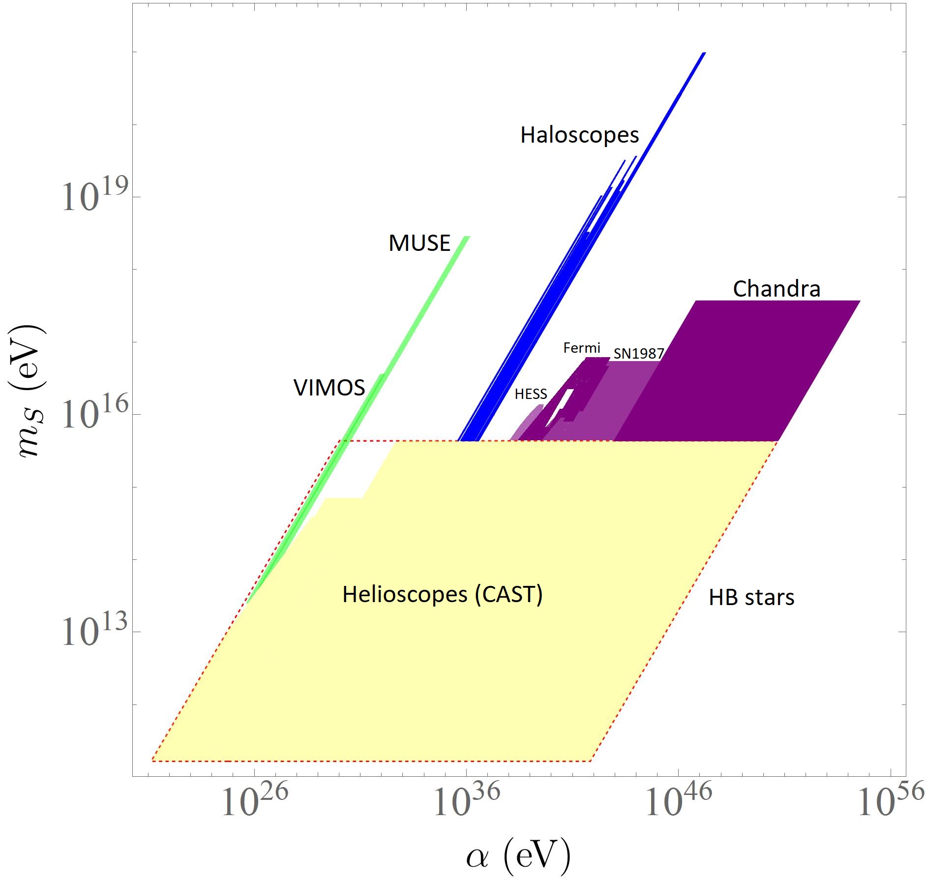
3) The coupling of ALPs with the electromagnetic sector, i.e. , has motivated most of the experimental searches for these kinds of particles, since such an interaction predicts the interconversion with photons in the presence of a background magnetic field [31]. The effects of this conversion can in principle be measured by several telescopes and ground-based experiments. Paradigmatic examples include (see [32]):
Helioscopes: These kinds of constraints are based on the assumption that the ALP is a constituent of our galactic halo. Hence, the Sun would be able to produce them, and the photons produced by passing a magnetic field would be detectable on Earth on the X-ray region. Following this reasoning, the most stringent values have been provided by the CERN experiment CAST, which gives an upper bound of the ALP-photon coupling of for a mass .
Haloscopes: These detectors are designed to measure microwave-photon signals from axions in our galactic halo. They are able to set the best constraints on the microwave range. Some experiments under this classification include RBF-UF, ADMX, HAYSTAC, CAPP, and for low-mass searches, ABRACADABRA and SHAFT.
Astrophysical measures: here we include the astrophysical observations that would be affected by ALPs. The study of globular clusters gives one of the strongest constraints for the large-mass range. The number count of Horizontal Branch stars (HB), which can produce axions by the Primakoff process, unlike the red giants, which are not affected by these losses, gives a bound of to the ALP-photon coupling in a wide mass range [33]. For small masses, the measure of X-ray sources with Chandra, gives one of the most stringent constraints. Also, the study of gamma rays from SN 1987A, and the active galactic nuclei of AGN PKS 2155-304 and NGC 1275 (by the HESS and Fermi-LAT collaborations respectively), gives comparable constraints. Finally, for large masses the best bounds are given by the spectroscopic observations of the dwarf spheroidal galaxy Leo T using the MUSE survey, in order to find ALP radiative decay, and of galaxy clusters Abell 2667 and 2390, using spectra from VIMOS.
A representation of the constraints above and the pertinent references to the experiments can be found in [32]. By using the relation between and , it can be easily seen that the limits imposed on in these studies turn to be stronger than the ones from the four-fermion contact interaction. We represent the experimental constraints derived from the electromagnetic coupling in the parameter space in Figure 1.
4) The coupling of ALPs to fermions, i.e., , produce spin flips in a magnetic sample placed inside a static magnetic field. Such spin flips would then emit radio-frequency photons that can be detected by a suitable quantum counter in an ultra-cryogenic environment [34]. Based on this effect,the QUAX experiments has put the strongest constraints on the strength of this coupling [35]. In particular, a constraint of is found for masses in the interval . This translates in a lower limit of for for the mentioned ALP mass range.
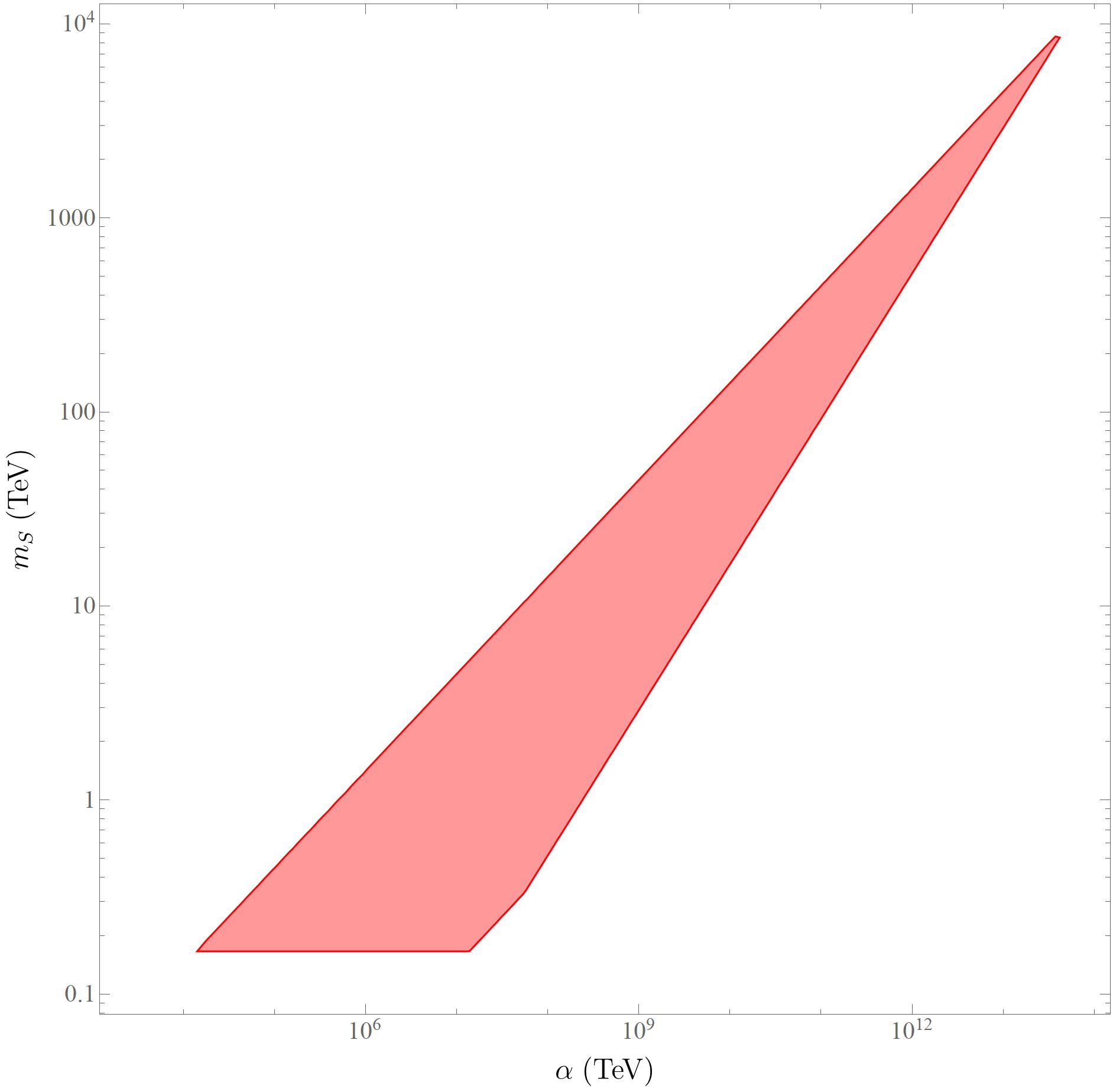
Finally, let us focus on ALPs constraints for ultralight and heavy masses. On the one hand, recent analysis of the Lyman-alpha forest searching for suppressed cosmic structure growth, have shown a lower limit on the mass of ultra-light axions of [36]. On the other hand, the upper limits on the mass of the particle are found based on decays to SM particles. Such a decay affects the abundance of light elements in the Universe, and hence it may affect the cosmological evolution. The ALP coupling with the electromagnetic sector allows ALPs to decay into two photons, with a lifetime [24]
| (9) |
If , where is the age of the Universe, then the ALP would be stable for the lifetime of the Universe. In the parameter space, such a condition translates to . Otherwise, the decay of the ALP would affect the cosmological evolution, and hence constraints can be imposed. In particular, it is found that the ALPs with the following range of masses and lifetimes are excluded [24]:
| (10) |
Such constraints have been translated to the parameter space in Figure 2.
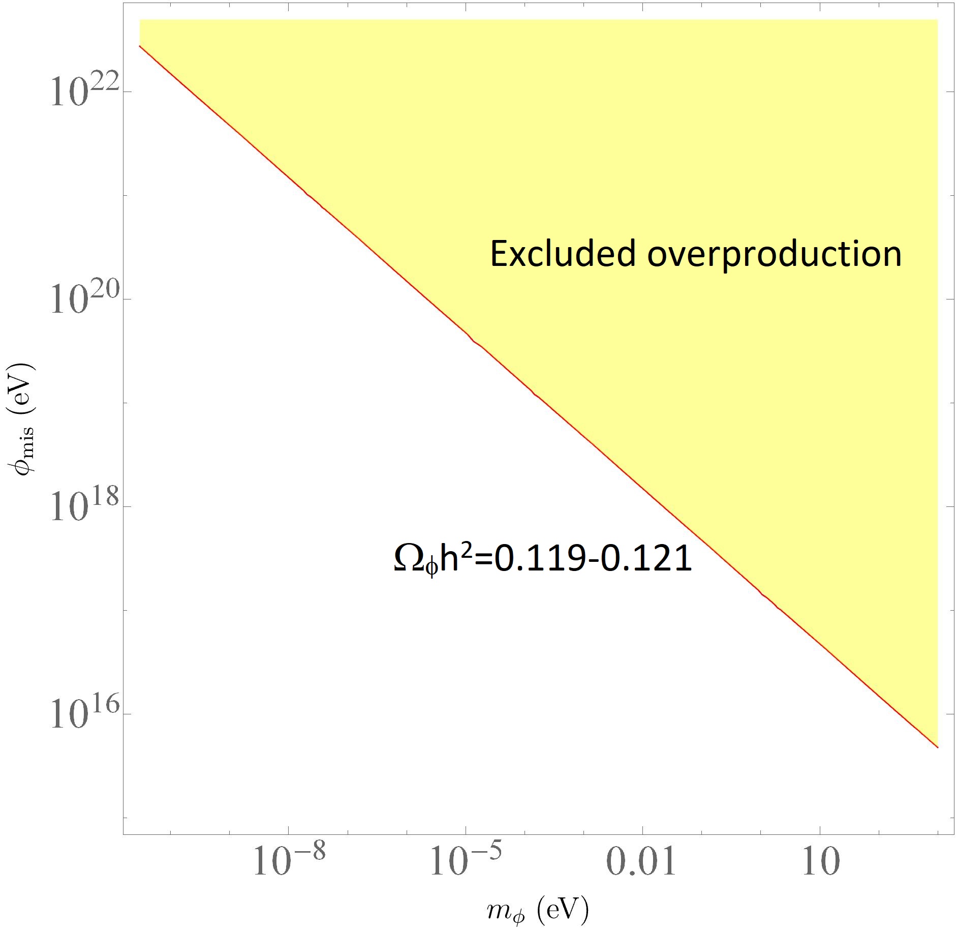
Describing CDM.— As we have established, the Poincaré Gauge gravity pseudo-scalar d.o.f. is an ALP. Provided that the experimental constraints are fulfilled, this predicted particle could serve as a DM candidate. Nevertheless, we have to make sure that the early Universe production of such a particle can account for the DM density measured by observations [37]. In order to perform the density calculation we assume that the production of the ALP is done via the misalignment mechanism. Such a mechanism relies on the fact that fields in the early Universe have a random initial state. After the mass of the particle is comparable to the Hubble parameter, the fields respond by attempting to minimise their potential, hence oscillating around the minimum. These oscillations can behave as CDM since their energy density is diluted by the expansion of the Universe as [38]. After studying the pseudo-scalar evolution in a Friedman-Lemaître-Robertson-Walker (FLRW) background, one can show that the production mechanism starts when . Hence, the relation between the Hubble parameter and the temperature in the radiation dominated era can be used to find the temperature at which the mechanism starts. Thus, knowing the temperature at which the mechanism begins to take place , we can calculate the expected density today from this production as [38]
| (11) |
where and are the effective numbers of energy and entropy d.o.f.s respectively [39]. Moreover, we have taken into account that in this case the ALP mass is constant, and we have used the value for the critical density of the Universe [23].
The most precise value for the CDM density today, , is given by the Planck Collaboration [37]. Hence, if we want the ALP to describe the entire dark matter content, we shall require . This implies that the initial value of the field after inflation imposes a very limited allowed mass range, and vice versa. Also, the values of and providing higher densities of dark matter would be of course excluded. These constraints are represented in Figure 3.
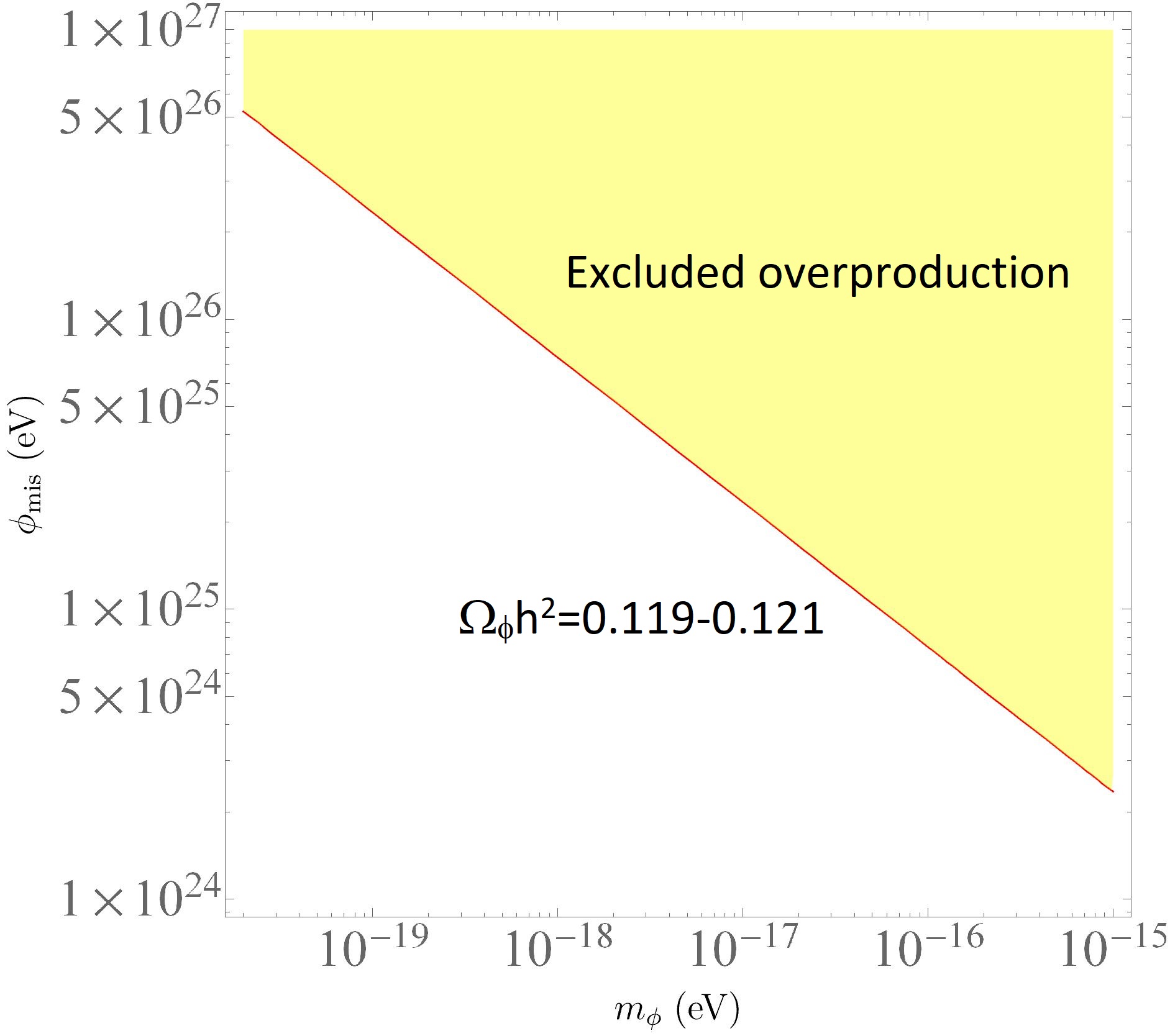
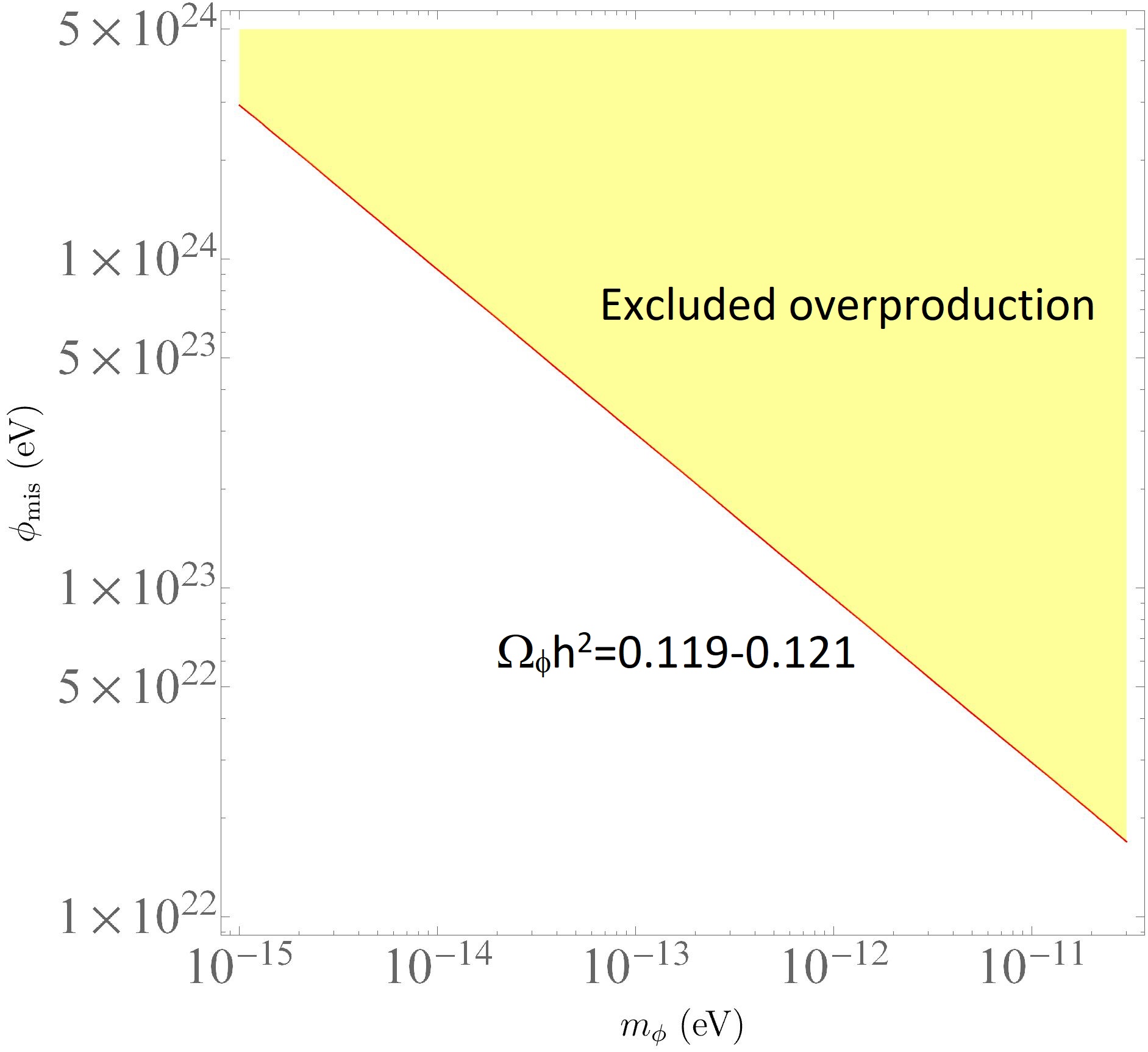
Furthermore, the constraints on would affect the possible values of if we require the weak-field limit approximation to be valid. Such an approximation requires that . Hence, from Figure 3 we can infer the possible values of such that the pseudo-scalar accounts for the whole cold dark matter while the weak-field limit is still applicable.
In conclusion, we show that the pseudo-scalar mode of Poincaré Gauge Gravity behaves like an axion-like particle. We find experimental constraints for the free parameters from the interactions present in the theory. Finally, we provide the conditions for which the pseudo-scalar mode present in this theory can account for the entirety of cold dark matter.
Acknowledgements.
We thank J. Beltrán Jiménez, J.A.R. Cembranos, and J. Gigante Valcarcel for helpful conversations. FJMT and AdlCD acknowledge support from NRF grants no.120390, reference:BSFP190416431035; no.120396, reference:CSRP190405427545; no.101775, reference: SFH150727131568. AdlCD acknowledges support from grants PID2019-108655GB-I00 and COOPB204064, I-COOP+2019, MICINN Spain. DFM and FJMT acknowledge support from the Research Council of Norway.References
- Riess et al. [1998] A. G. Riess et al. (Supernova Search Team), Astron. J. 116, 1009 (1998).
- Sahni [2004] V. Sahni, Lect. Notes Phys. 653, 141 (2004), eprint astro-ph/0403324.
- Peebles and Ratra [2003] P. J. E. Peebles and B. Ratra, Rev. Mod. Phys. 75, 559 (2003), eprint astro-ph/0207347.
- Weinberg [1989] S. Weinberg, Rev. Mod. Phys. 61, 1 (1989).
- Bertone et al. [2005] G. Bertone, D. Hooper, and J. Silk, Phys. Rept. 405, 279 (2005), eprint hep-ph/0404175.
- Cembranos [2009] J. A. R. Cembranos, Phys. Rev. Lett. 102, 141301 (2009), eprint 0809.1653.
- Clifton et al. [2012] T. Clifton, P. G. Ferreira, A. Padilla, and C. Skordis, Phys. Rept. 513, 1 (2012), eprint 1106.2476.
- Amendola et al. [2018] L. Amendola et al., Living Rev. Rel. 21, 2 (2018), eprint 1606.00180.
- Blagojević and Hehl [2013] M. Blagojević and F. W. Hehl, eds., Gauge Theories of Gravitation: A Reader with Commentaries (World Scientific, Singapore, 2013), ISBN 978-1-84816-726-1.
- Ponomarev et al. [2017] V. N. Ponomarev, Y. V. Obukhov, and A. Barvinsky, Gauge approach and quantization methods in gravity theory (Nauka, 2017).
- Hayashi and Shirafuji [1980] K. Hayashi and T. Shirafuji, Prog. Theor. Phys. 64, 2222 (1980).
- Yo and Nester [1999] H.-j. Yo and J. M. Nester, Int. J. Mod. Phys. D 8, 459 (1999), eprint gr-qc/9902032.
- Yo and Nester [2002] H.-J. Yo and J. M. Nester, Int. J. Mod. Phys. D 11, 747 (2002), eprint gr-qc/0112030.
- Jiménez and Maldonado Torralba [2020] J. B. Jiménez and F. J. Maldonado Torralba, Eur. Phys. J. C 80, 611 (2020), eprint 1910.07506.
- Hojman et al. [1980] R. Hojman, C. Mukku, and W. Sayed, Phys. Rev. D 22, 1915 (1980).
- Holst [1996] S. Holst, Phys. Rev. D53, 5966 (1996), eprint gr-qc/9511026.
- Castellani et al. [1991] L. Castellani, R. D’auria, and P. Fre, Supergravity and superstrings: a geometric perspective (in 3 volumes), vol. 1 (World Scientific Publishing Company, 1991).
- Taveras and Yunes [2008] V. Taveras and N. Yunes, Phys. Rev. D78, 064070 (2008), eprint 0807.2652.
- Calcagni and Mercuri [2009] G. Calcagni and S. Mercuri, Phys. Rev. D79, 084004 (2009), eprint 0902.0957.
- Torres-Gomez and Krasnov [2009] A. Torres-Gomez and K. Krasnov, Phys. Rev. D 79, 104014 (2009), eprint 0811.1998.
- Mercuri [2009] S. Mercuri, Phys. Rev. Lett. 103, 081302 (2009), eprint 0902.2764.
- Shapiro [2002] I. L. Shapiro, Phys. Rept. 357, 113 (2002), eprint hep-th/0103093.
- Zyla et al. [2020] P. A. Zyla et al. (Particle Data Group), PTEP 2020, 083C01 (2020).
- Marsh [2016] D. J. E. Marsh, Phys. Rept. 643, 1 (2016), eprint 1510.07633.
- Bertlmann [1996] R. A. Bertlmann, Anomalies in quantum field theory (1996).
- Zarnecki [1999] A. F. Zarnecki, Eur. Phys. J. C 11, 539 (1999), eprint hep-ph/9904334.
- Alexander and Yunes [2009] S. Alexander and N. Yunes, Phys. Rept. 480, 1 (2009), eprint 0907.2562.
- Jung et al. [2020] S. Jung, T. Kim, J. Soda, and Y. Urakawa, Phys. Rev. D 102, 055013 (2020), eprint 2003.02853.
- Yunes and Pretorius [2009] N. Yunes and F. Pretorius, Phys. Rev. D 79, 084043 (2009), eprint 0902.4669.
- Ali-Haimoud and Chen [2011] Y. Ali-Haimoud and Y. Chen, Phys. Rev. D 84, 124033 (2011), eprint 1110.5329.
- Chadha-Day et al. [2021] F. Chadha-Day, J. Ellis, and D. J. E. Marsh, Axion Dark Matter: What is it and Why Now? (2021), eprint 2105.01406.
- Semertzidis and Youn [2021] Y. K. Semertzidis and S. Youn, Axion Dark Matter: How to detect it? (2021), eprint 2104.14831.
- Ayala et al. [2014] A. Ayala, I. Domínguez, M. Giannotti, A. Mirizzi, and O. Straniero, Phys. Rev. Lett. 113, 191302 (2014), eprint 1406.6053.
- Barbieri et al. [2017] R. Barbieri, C. Braggio, G. Carugno, C. S. Gallo, A. Lombardi, A. Ortolan, R. Pengo, G. Ruoso, and C. C. Speake, Phys. Dark Univ. 15, 135 (2017), eprint 1606.02201.
- Crescini et al. [2020] N. Crescini et al. (QUAX), Phys. Rev. Lett. 124, 171801 (2020), eprint 2001.08940.
- Rogers and Peiris [2021] K. K. Rogers and H. V. Peiris, Phys. Rev. Lett. 126, 071302 (2021), eprint 2007.12705.
- Aghanim et al. [2020] N. Aghanim et al. (Planck), Astron. Astrophys. 641, A6 (2020), [Erratum: Astron.Astrophys. 652, C4 (2021)], eprint 1807.06209.
- Arias et al. [2012] P. Arias, D. Cadamuro, M. Goodsell, J. Jaeckel, J. Redondo, and A. Ringwald, JCAP 06, 013 (2012), eprint 1201.5902.
- Husdal [2016] L. Husdal, Galaxies 4, 78 (2016), eprint 1609.04979.