Dark Matter CMB Constraints and Likelihoods
for Poor Particle Physicists

The temperature and polarization fluctuations of the cosmic microwave background (CMB) are well known to be sensitive to the redshift of recombination, $z\approx 1100$, as this determines the surface of last scattering. If dark matter annihilation or decay deposits electromagnetic energy in the primordial plasma after $z\approx 1100$, it can delay recombination and/or contribute to reionization, leading to distortions in the CMB Dodelson:1991bz ; Scott91 ; Hansen:2003yj ; Chen:2003gz ; Padmanabhan:2005es ; Mapelli:2006ej ; Zhang:2007zzh ; Natarajan:2009bm ; Galli:2009zc ; Slatyer:2009yq ; Galli:2011rz ; Cirelli:2009bb ; Hutsi:2011vx ; Finkbeiner:2011dx ; Natarajan:2012ry ; Giesen:2012rp ; Slatyer:2012yq ; Frey:2013wh ; Weniger:2013hja . This is especially constraining for light dark matter $\chi$ with mass $m_{\chi}\lesssim$ 10 GeV (as its number density is greater than that of heavier dark matter), and if annihilation or decay is into electrons; in that case the current limit on the annihilation cross section is close to the standard relic density value $\langle\sigma v\rangle=3\times 10^{-26}$ cm³/s. Apart from the special case of monochromatic photons, constraints are generically weaker for annihilations or decays into other particles, as those channels all involve substantial eventual yields into neutrinos and/or hadrons, neither of which efficiently transfer energy to the primordial gas (neutrinos because they are weakly-interacting, hadrons because they are strongly penetrating Chen:2003gz ).

Recent progress has been made in refining and systematizing the CMB bounds on dark matter annihilation and decay Finkbeiner:2011dx ; Slatyer:2012yq . A key quantity for determining the constraint on a given model is the efficiency $f(z)$ for producing ionizing radiation, as a function of redshift $z$. For annihilations, $f(z)$ is defined in terms of the electromagnetic power injected per unit volume,

$${dE\over dt\,dV}=f(z){\langle\sigma v\rangle\over m_{\chi}}\,\Omega_{\rm DM}^{2}\,\rho_{c}^{2}\,c^{2}\,(1+z)^{6},$$

(1)

where $\rho_{c}$ is the critical mass density of the universe today and $\Omega_{\rm DM}$ is the fraction in dark matter. For perfect efficiency, $f=1$, this is just twice the the DM mass times the annihilation rate per unit volume. Note that no factors of two remain in (1), as the annihilation rate itself contains a factor of one half for annihilation of identical particles Gondolo:2004sc , which cancels the factor of two from the release of twice the DM rest mass in each annihilation event. Here we assume Majorana DM; were the DM not its own antiparticle, (1) would need to be divided by a further factor of two, and $\Omega_{\rm DM}$ interpreted as the total mass fraction of DM $+$ anti-DM particles.

Ref. Slatyer:2012yq has provided transfer functions $T_{i}(z^{\prime},z,E)$¹¹1Available at http://nebel.rc.fas.harvard.edu/epsilon/ that determine the contribution to $f(z)$ from particles $i=\gamma$ or $e^{\pm}$ pairs injected at redshift $z^{\prime}$ with energy $E$. The injected $\gamma$ or $e^{\pm}$ may be primary products of dark matter annihilation or decay, or they may be secondary particles arising from the showering and decay of the primary ones. If $\phi_{i}=dN_{i}/dE$ is the electron/photon spectrum of state $i$, normalized such that $\int dE\,E\,\phi_{i}$ is the fraction of initial dark matter mass converted into energy in that state, then²²2Our $\tilde{T}_{i}$ is related to $T_{i}$ of Slatyer:2012yq by $\tilde{T}_{i}=H(z)H(z^{\prime})^{-1}(1+z^{\prime})^{n}(1+z)^{-(n+1)}T_{i}$, where $n=2$ for annihilations and $n=-1$ for decays.

$$f(z)=\sum_{i=\gamma,\,e^{\pm}}\int dz^{\prime}\int dE\,E\,\tilde{T}_{i}(z^{\prime},z,E)\,\phi_{i}(E).$$

(2)

The departure from perfect efficiency, $f=1$, is due to the fraction of initial energy that ends up in neutrinos (or possibly more exotic invisible final states, which we do not explicitly consider here).

To find the spectra $\phi_{i}$, Monte Carlo computations using an event generator such as PYTHIA Bengtsson:1987kr ; Sjostrand:2007gs or HERWIG Corcella:2000bw are required. These simulations are numerically intensive, but the results have been carried out and made available for a range of primary annihilation and decay channels in ref. Cirelli:2010xx . The spectra obtained from PYTHIA 8.135 and HERWIG 6.510 generally agree to within about 20% for most primary annihilation/decay channels, except for $g$ (gluons), where the choice of event generator results in up to a factor of two uncertainty in electron and photon yields. At lower energies PYTHIA also gives substantially larger photon yields for leptonic and gauge boson channels, a consequence of the omission of (QED) lepton final state radiation and fermion pair production in HERWIG. We therefore exclusively employ the PYTHIA results of ref. Cirelli:2010xx , which have the additional benefit of also including electroweak corrections Ciafaloni .

The purpose of the present note is to provide a set of results that can be easily interpolated to find CMB constraints and likelihood functions for dark matter models that annihilate or decay to arbitrary final states with a constant cross-section or decay rate. We first carry out the computation of (2) for a full range of dark matter masses and annihilation and decay channels, and then translate each result into a single number that encodes the energy injection history for that mass and final state. For annihilation we use $f_{\rm eff}$, the effective efficiency of energy injection, whereas for decays we define an alternative quantity $\eta$. We then detail how likelihoods and corresponding constraints are obtained as a function of $f_{\rm eff}$ or $\eta$, including a simple prescription for combining results from multiple channels.

Here we explicitly build upon existing public datasets Finkbeiner:2011dx ; Slatyer:2012yq ; Cirelli:2010xx , adding the necessary final steps for earlier results to be immediately implemented in, for example, multi-messenger dark matter analyses Pato:2009fn and global fits to beyond the Standard Model particle theories Bechtle:2012zk ; Buchmueller:2012hv ; Strege:2012bt . This complements and extends recent efforts to construct public likelihood functions from Fermi-LAT Scott:2009jn , HESS Ripken:2010ja and IceCube Scott:2012mq searches for dark matter annihilation.

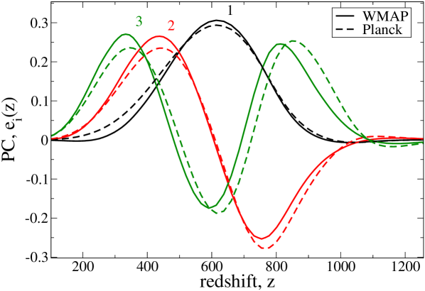
Annihilating dark matter. We will first consider the case of dark matter annihilating into standard model particles. Bounds on annihilation cross sections can be encoded in an integral involving $f(z)$ and a set of principal component basis functions $e_{i}(z)$ that should be optimized for annihilations, and which depend somewhat upon which experiment is being considered since they are eigenvectors of the Fisher matrix. As discussed in Finkbeiner:2011dx ; Slatyer:2012yq , $f(z)$ can be expanded as

$$\varepsilon\,f(z)=\sum_{i=1}^{\infty}{\varepsilon_{i}}e_{i}(z)$$

(3)

where $\varepsilon\equiv\langle\sigma v\rangle/m_{\chi}$ and $\varepsilon_{i}=\varepsilon\,f(z)\!\cdot\!\,e_{i}(z)/e_{i}(z)\!\cdot\!\,e_{i}(z)$. The inner product is the integral over $z$ using the integration limits $z_{1}=86.83$, $z_{2}=1258.2$. For annihilating dark matter, these basis functions are chosen to maximize sensitivity to a general expected $z$-dependence for energy injection from annihilating dark matter, (based upon the energy density $(1+z)^{3}\Omega_{\rm DM}\rho_{c}c^{2}$ of the dark matter itself) in the sense that the most important contributions to the observable energy deposition are described by the lowest components. The first three $e_{i}(z)$ are plotted in fig. 1.

In fact, the contribution of the first component has been demonstrated to dominate, especially in the case of WMAP data, in the computation of the likelihood function that is relevant for constraining annihilating dark matter models. Under the approximation of a Gaussian likelihood, and that the response of the CMB to the energy injection is linear, the chi-squared is given by Finkbeiner:2011dx ; Slatyer:2012yq

$$\Delta\chi^{2}=\sum_{i}\lambda_{i}\varepsilon_{i}^{2}/\bar{\varepsilon}^{2}$$

(4)

where $\lambda_{i}$ is the eigenvalue of the Fisher matrix corresponding to $e_{i}$, for the relevant CMB experiment, and $\bar{\varepsilon}$ is a fiducial value, taken to be $2\times 10^{-27}$ cm${}^{3}\,$s${}^{-1}\,$GeV^-1. For WMAP7, $\lambda_{1}=0.279$, while for Planck, $\lambda_{i}=3.16,\,0.691,\,0.162\dots$, and the inclusion of contributions from the first three principal components is justified. Then, for example, the $2\sigma$ upper limit on the cross section is given by

$$\langle\sigma v\rangle<{2m_{\chi}\bar{\varepsilon}\over\sqrt{\sum_{i}\lambda_{i}((f\cdot e_{i})/(e_{i}\cdot e_{i}))^{2}}}$$

(5)

The numerical value of the numerator in (5) (as well as that of (6) below) is correlated with the choice of normalization of the $e_{i}(z)$’s. We use the functions shown in fig. 1, which are normalized such that $(e_{i}\cdot e_{i})=23.9$.

However, it was observed in ref. Finkbeiner:2011dx that the approximation of linear response is not yet very accurate for the magnitudes of $\varepsilon_{i}$ that are allowed by the WMAP7 data; instead one should perform a full likelihood analysis using CosmoMC Lewis:2002ah (and it is found that only the first principal component is required). This gives a somewhat weaker constraint than (5); the 95% c.l. upper bound is

$$\langle\sigma v\rangle<1.2\times 10^{-26}{{\rm cm}^{3}\over{\rm s\cdot GeV}}\,{m_{\chi}\over(f\cdot e_{1})/(e_{1}\cdot e_{1})}$$

(6)

(Throughout this paper, we use “95% c.l.” to mean $2\sigma$, which is in fact 95.45% c.l..)

In either (5) or (6), we see that the constraints can be expressed in terms of a single number involving integrals of $f(z)$. To make contact with the earlier literature Slatyer:2009yq , we find it useful to consider a quantity $f_{\rm eff}$ defined in terms of a “universal WIMP annihilation” curve $e_{\scriptscriptstyle\rm W}(z)$ Finkbeiner:2011dx , $f_{\rm eff}\sim(f\cdot e_{\scriptscriptstyle\rm W})/(e_{\scriptscriptstyle\rm W}\cdot e_{\scriptscriptstyle\rm W})$, which has the interpretation that $f_{\rm eff}<1$ denotes the average efficiency of energy injection for the annihilation channel of interest. It can be compared to the $f_{\rm mean}$ values tabulated in ref. Slatyer:2009yq (column 2, table I). Here instead of defining $f_{\rm eff}$ directly in terms of $e_{\scriptscriptstyle\rm W}$, we use the expansion $e_{\scriptscriptstyle\rm W}=\sum_{i}c_{i}e_{i}$, and the observation that using just the first term in the expansion gives a good approximation. Thus for WMAP7 we define

$$f_{\rm eff}\equiv{(f\cdot e_{1})\over c_{1}(e_{1}\cdot e_{1})}\qquad{\rm(WMAP)}$$

(7)

where numerically $c_{1}=4.64$. Then (6) can be expressed as

$$\langle\sigma v\rangle<0.26\times 10^{-26}\,{\rm cm}^{3}\,{\rm s}^{-1}\,{\rm GeV}^{-1}m_{\chi}/f_{\rm eff}.$$

(8)

The analogous definition for Planck, which makes use of the contributions from the first three principal components, is

$$f_{\rm eff}\equiv{1\over\sqrt{\lambda_{1}}c_{1}}\left[\sum_{i}\lambda_{i}\left({f\cdot e_{i}\over e_{i}\cdot e_{i}}\right)^{2}\right]^{1/2}\quad({\rm Planck})$$

(9)

where we must use the $\lambda_{i}$ and $e_{i}$ appropriate to Planck. Then the 2$\sigma$ projected constraint from Planck takes the form $\langle\sigma v\rangle<0.48\times 10^{-27}\,{\rm cm}^{3}\,{\rm s}^{-1}\,{\rm GeV}^{-1}m_{\chi}/f_{\rm eff}$. For annihilation into several channels $i$ with branching fractions $r_{i}$, the total $f_{\rm eff}$ is

$$f_{\rm eff}=\sum_{i}r_{i}f_{{\rm eff},i}.$$

(10)

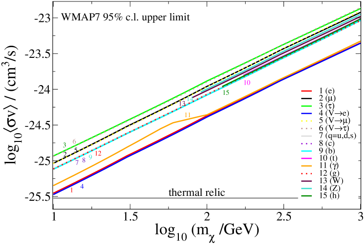
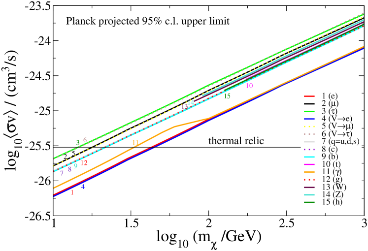
We present the 95% CL constraints as a function of $m_{\chi}$ for a range of annihilation channels in fig. 2, interpolating from table 1. The final states are pairs of $e$, $\mu$, $\tau$, $V\to e,$³³3$V\to X$ denotes $\chi\chi\to VV$ followed by $V\to X\bar{X}$ with $m_{V}=1$ GeV for $X=e$ or $\mu$ and $m_{V}=5$ GeV for $X=\tau$. $V\to\mu$, $V\to\tau$, $q$ (light quarks: $u,d$ or $s$), $c$, $b$, $t$, $W$, $Z$, $g$ (gluons), $\gamma$, or $h$ (Higgs). The limits from WMAP7 and projected constraints from Planck based on 14 months of observation time Planck:2006aa are shown in the figure. Our 95% C.L. WMAP7 limits perfectly match those for $e$ and $\mu$ found in present benchmark results (e.g. at $m_{\chi}=100$ GeV, $\langle\sigma v\rangle<4\times 10^{-25}$ cm³ s^-1 for $e^{+}e^{-}$, $\langle\sigma v\rangle<1\times 10^{-24}$ cm³ s^-1 for $\mu^{+}\mu^{-}$ Galli:2011rz ; Finkbeiner:2011dx ). We see approximately a factor of 6 improvement between WMAP7 and Planck, in agreement with the results of Hutsi:2011vx but slightly less than the factor of 8 reported by Galli:2011rz .

Limits are strongest on the channels $[e,\,V\to e]$ (which in fact coincide) and $\gamma$, which also coincides with the former at masses $\gtrsim 100$ GeV. The $\gamma\gamma$ final state limit has a different shape from the others because of the monochromatic nature of the photons and the complex dependence of the efficiency of photon energy deposition on redshift and injection energy. This is encoded in the transfer function $\tilde{T}_{\gamma}$, and can be seen for example in fig. 1 of Slatyer:2012yq and fig. 2 of Chen:2003gz . At redshifts of $z\sim 600$, where the first principal component of fig. 1 is peaked, the Universe is approximately transparent to photons with energies $E\lesssim 50\,$GeV, but rapidly transitions to completely opaque for $E\gtrsim 100\,$GeV, due to scattering and pair production on CMB photons Chen:2003gz . This causes the $\gamma\gamma$ curve to track the electron curve above 100 GeV, as in both cases essentially all of the annihilation energy goes into heating the primordial gas. The $\gamma\gamma$ channel is the only one in which photons dominate over electrons in the final state spectra, and the only one to produce monochromatic photons – so it is the only one to show this complicated behaviour in the limits.

The next strongest constraints are on the channels involving quarks, gluons and Higgs. These all coincide with each other (except that the top quark and Higgs have a higher mass threshold). The next weakest constraints are on $[W,\,Z]$, followed by $[\mu,\,V\to\mu]$ and finally $[\tau,\,V\to\tau]$. These tendencies are indicative of the greater fraction of energy ending up in neutrinos for the least constrained channels.

We stress that our results do not depend in any intrinsic way upon the somewhat arbitrary definitions (7,9). Any quantity proportional to $f\cdot e_{1}$ in the case of WMAP or $(\sum_{i}\lambda_{i}(f\cdot e_{i}/e_{i}\cdot e_{i})^{2})^{1/2}$ in the case of Planck would suffice to encode the necessary information for recovering the constraints. To this end, we list $f_{\rm eff}$ values for both WMAP and Planck in table 1, for the annihilation channels mentioned above and for the WIMP masses $m_{\chi}=10,\,30,\,100,\,300,\,1000$ GeV. They are in reasonable agreement with the $f_{\rm mean}$ values tabulated in ref. Slatyer:2009yq in the cases that overlap.

To determine constraints at an arbitrary confidence level, one would like to know the likelihood function for the annihilation cross section, assuming branching fractions $r_{i}$ to channel $i$. For Planck, this is given by

$$\begin{split}\ln\,&\mathcal{L}(\langle\sigma v\rangle|m_{\chi},r_{i})=\\ &-\frac{1}{2}f_{\rm eff}^{2}(m_{\chi},r_{i})\lambda_{1}c_{1}^{2}\,\left(\frac{\langle\sigma v\rangle}{2\times 10^{-27}{\rm cm}^{3}{\rm s}^{-1}}\right)^{2}\,\left(\frac{\rm GeV}{m_{\chi}}\right)^{2}.\\ \end{split}$$

(11)

from (5) and (9). As mentioned above, this expression, which assumes linear response of the CMB to the deposited energy, is not accurate for WMAP. This can be corrected by making the replacement $2\times 10^{-27}\to 3.2\times 10^{-27}$ in (LABEL:loglike2) (and one must also use the appropriate value $\lambda_{1}=0.279$ for WMAP). Similarly, caution should be exercised if (LABEL:loglike2) is used to compute WMAP likelihoods far from 95% c.l.  as the Gaussian approximation was observed to be poor for WMAP likelihoods in ref. Finkbeiner:2011dx . The WMAP 7-year limits can also be improved by $\sim$15% if ACT data are added to the CosmoMC fit Galli:2011rz , and presumably slightly more than this if SPT data are added.

Decaying dark matter. A similar procedure can be used to constrain the fractional mass abundance $\delta\Omega$ of some metastable species present at the time of recombination, which decays into the same set of final states as we assumed above for annihilations. If the decaying species originally contributes $\Omega_{i}$ to the mass density of the universe relative to $\rho_{c}$, and if the decay of a particle of that species converts a fraction $\phi$ of its rest mass to standard model particles (and a fraction $1-\phi$ to some lighter dark species), then $\delta\Omega=\phi\Omega_{i}$. The injected electromagnetic power density goes as

$${dE\over dt\,dV}={f(z)\over\tau}\,e^{-t/\tau}\,\delta\Omega\,\rho_{c}\,c^{2}\,(1+z)^{3}.$$

(12)

The factor of $(1+z)^{3}\sim n_{\chi}$ as opposed to $(1+z)^{6}\sim n_{\chi}^{2}$ for annihilations is the reason for the different powers of $(1+z)$ appearing in footnote 2. Unlike the case of annihilation, where the cross section appears only as a prefactor, here we have dependence upon the lifetime $\tau$ not only in the prefactor, but also in the $z$-dependent function $e^{-t(z)/\tau}$, which is not present in (1). This makes the analysis of decays more cumbersome than that of annihilations, because the transfer functions $\tilde{T}_{i}(z^{\prime},z,E)$ now also depend upon $\tau$. We therefore need to compute (2) not only for all masses and final states, but for a grid of lifetimes as well.

Note that this form of analysis allows us to not only constrain the lifetime and abundance of decaying dark matter candidates, but also the initial abundance of other metastable species, with such short lifetimes that they would not contribute to the current-day abundance of dark matter. For lifetimes less than $\sim$$10^{17}$–$10^{18}$ s the particles we refer to are therefore not dark matter in the usual sense, but rather some generic metastable particles.

In the approximation of linear response to the injected energy, the chi-squared is most conveniently written in the form Slatyer:2012yq

$$\Delta\chi^{2}=\left(\delta\Omega\over\Omega_{\rm DM}\tau\right)^{2}\eta^{2},$$

(13)

where we define

$$\eta=\left[\sum_{i}\left({(f\cdot e_{i})\over(e_{i}\cdot e_{i})\,\sigma_{i}}\right)^{2}\right]^{1/2}$$

(14)

to be the single number that encapsulates the energy injection history for a given mass, lifetime and final state (as $f_{\rm eff}$ does for annihilation). The likelihood is then simply

$$\ln\,\mathcal{L}(\tau|m_{\chi},r_{i})=-\frac{1}{2}\left(\delta\Omega\over\Omega_{\rm DM}\tau\right)^{2}\eta^{2}(\tau,m_{\chi},r_{i}).$$

(15)

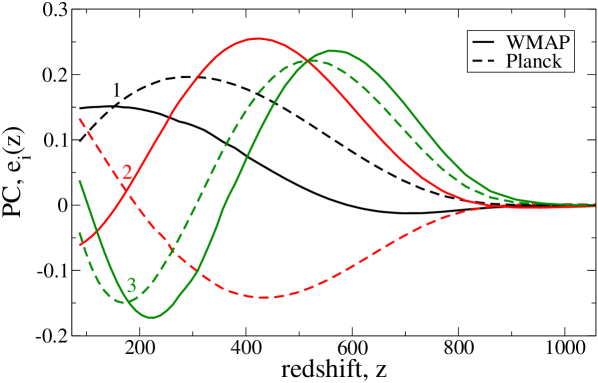
The principal components $e_{i}(z)$ in $\eta$ are now specialized to the case of decays, as well as depending upon the experiment. In contrast to annihilations, the first three components are needed for good accuracy, even for WMAP. We plot them for both experiments in fig. 3. The variances are given by $\sigma_{i}=(5.3,\,6.4,\,9.5\dots)\times 10^{-25}\,$s^-1 for WMAP7 and $(1.2,\,1.6,\,2.3\dots)\times 10^{-25}\,$s^-1 for Planck Slatyer:2012yq . The limits of integration appearing in $f\cdot e_{i}$ are $z_{1}=10$, $z_{2}=1258.2$, because $n_{\chi}$ redshifts slower than $n_{\chi}^{2}$, so lower redshifts are needed than in the case of annihilations. The inner products (and therefore the limits of integration) are now defined in terms of integrals over $\ln z$ rather than $z$, with normalization $(e_{i}\cdot e_{i})=0.0543$.

Like $f_{\rm eff}$, $\eta$ can be easily obtained for arbitrary branching fractions $r_{i}$ into multiple final states by taking the appropriate linear combination of values for single channels $\eta_{i}$

$$\eta=\sum_{i}r_{i}\eta_{i}.$$

(16)

We have computed $\eta$ for each of the 15 final states that were considered as annihilation channels in the previous section, over a grid of metastable particle masses $10,30,100,300,1000$ GeV as before (we augment this selection in the $\gamma$, $t$, $W$, $Z$ and $h$ channels where it would otherwise be too sparse), and a grid of 15 lifetimes. The results are given in table 2. For the $b$ channel, our results extend only as low as $m_{\chi}=12$ GeV, as all yields of Cirelli:2010xx for the $b$ channel go to zero as the energies of the the decay products approach 5 GeV (presumably because the $b$ mass was approximated to 5 GeV in the calculations of Cirelli:2010xx ).

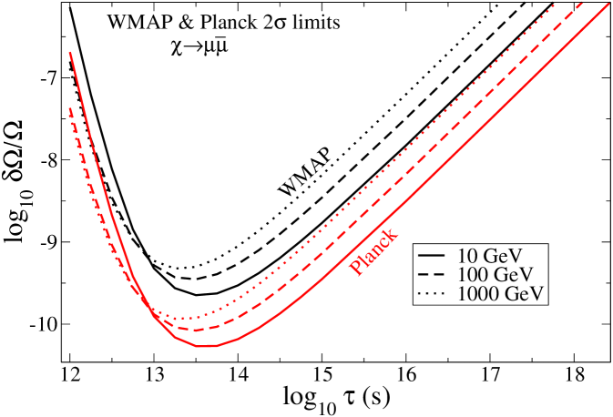
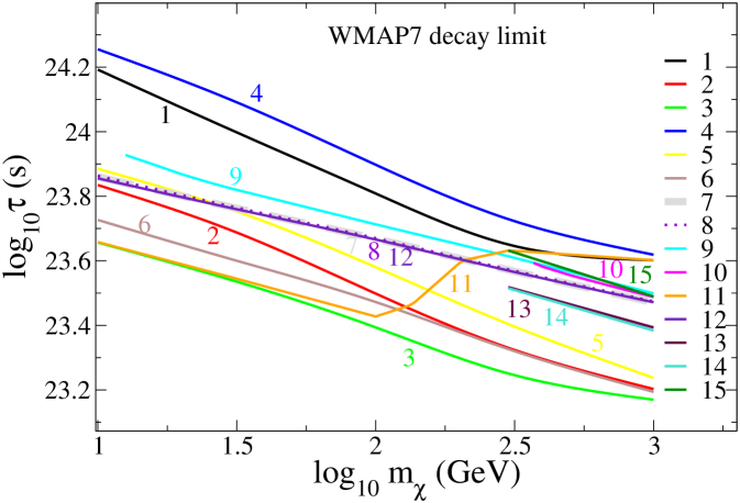
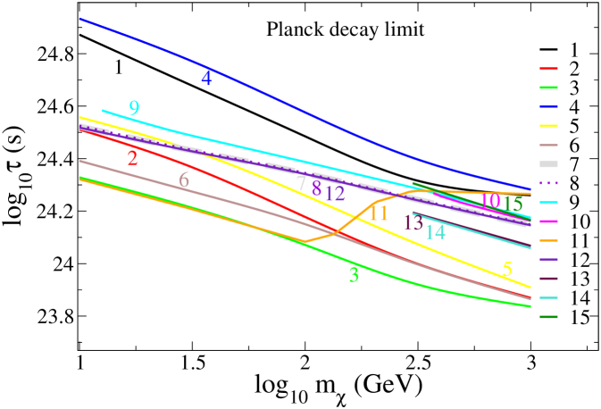
Our lifetime grid is sufficiently dense to show the structure of the limit on $\delta\Omega$ as a function of $\tau$. For longer lifetimes, $\eta$ is the same as the values we give for $\tau=10^{17}$, allowing constraints and likelihoods to be extended to arbitrarily long lifetimes. An example of the resulting constraints is given in fig. 4 for the $\chi\to\mu\bar{\mu}$ channel. Our results for other channels agree with those presented by Slatyer Slatyer:2012yq (as expected, given that we adopt her transfer functions here). In fig. 5 we plot the lower limit on the lifetime of a dark matter species decaying into any of the channels under consideration, assuming that it constitutes the entire presently-observed DM density.

We again added extra points to the mass grid for the $\gamma$ channel, in order to resolve the somewhat sharp feature seen in the region $100\lesssim m_{\chi}\lesssim 300$ GeV, as discussed previously in the results for annihilating dark matter. Note here that the mass range of the transition is approximately a factor of two larger than seen in annihilation (as decays produce photons with energies equal to half the DM mass), but that this factor is not exact because the redshifts of importance differ in the two cases, so the energy above which the Universe is opaque to photons injected at relevant redshifts differs slightly.

Our results for decaying species are based on the Fisher-matrix analysis of Finkbeiner:2011dx ; Slatyer:2012yq , which assumes that the linear approximation for the response of the CMB to energy injection at high redshift holds. Given the small ionization fraction at the redshifts most important for decay (at least when the lifetime is long) we do not expect nonlinear corrections to be crucial. In principle though, this assumption needs to be verified, for example with explicit CosmoMC calculations, as was done for annihilation.

It is also worth noting that the principal components $e_{i}(z)$ that we use for decay have been optimized for long decay lifetimes, leading to large leading contributions at relatively low redshift (fig. 3). In principle the $e_{i}(z)$ could also be optimized for different decay lifetimes, such that the optimal components for shorter lifetimes would probably begin to resemble those for annihilation to some degree (fig. 1), potentially allowing the limits we give here to be improved for the shortest lifetimes.

With tables 1 and 2, and eqs. LABEL:loglike2 and 15, we have provided a fast and easy means for implementing CMB constraints and likelihoods in future analyses of annihilating and decaying dark matter models, as well as some models with metastable particles that do not constitute dark matter. Our results can be interpolated to provide likelihood functions and limits for arbitrary particle masses, and arbitrary annihilation and decay final state mixtures.

References

- (1) D. Scott, M. J. Rees, D. W. Sciama, Astron. Astrophys. 250, 295, (1991).
- (2) S. Dodelson and J. M. Jubas, Phys. Rev. D 45, 1076 (1992).
- (3) S. H. Hansen and Z. Haiman, Astrophys. J. 600, 26 (2004) [astro-ph/0305126].
- (4) X. -L. Chen and M. Kamionkowski, Phys. Rev. D 70, 043502 (2004) [astro-ph/0310473].
- (5) N. Padmanabhan and D. P. Finkbeiner, Phys. Rev. D 72, 023508 (2005) [astro-ph/0503486].
- (6) M. Mapelli, A. Ferrara and E. Pierpaoli, Mon. Not. Roy. Astron. Soc. 369, 1719 (2006) [astro-ph/0603237].
- (7) L. Zhang, X. Chen, M. Kamionkowski, Z. Si and Z. Zheng, Phys. Rev. D 76, 061301 (2007) [arXiv:0704.2444].
- (8) A. Natarajan and D. J. Schwarz, Phys. Rev. D 80, 043529 (2009) [arXiv:0903.4485].
- (9) S. Galli, F. Iocco, G. Bertone and A. Melchiorri, Phys. Rev. D 80, 023505 (2009) [arXiv:0905.0003].
- (10) T. R. Slatyer, N. Padmanabhan and D. P. Finkbeiner, Phys. Rev. D 80, 043526 (2009) [arXiv:0906.1197].
- (11) M. Cirelli, F. Iocco and P. Panci, JCAP 0910 (2009) 009 [arXiv:0907.0719].
- (12) G. Hutsi, J. Chluba, A. Hektor and M. Raidal, Astron. Astrophys. 535, A26 (2011) [arXiv:1103.2766].
- (13) S. Galli, F. Iocco, G. Bertone and A. Melchiorri, Phys. Rev. D 84, 027302 (2011) [arXiv:1106.1528].
- (14) D. P. Finkbeiner, S. Galli, T. Lin and T. R. Slatyer, Phys. Rev. D 85, 043522 (2012) [arXiv:1109.6322].
- (15) A. Natarajan, Phys. Rev. D 85, 083517 (2012) [arXiv:1201.3939].
- (16) G. Giesen, J. Lesgourgues, B. Audren and Y. Ali-Haimoud, JCAP 1212, 008 (2012) [arXiv:1209.0247].
- (17) T. R. Slatyer, arXiv:1211.0283.
- (18) A. R. Frey and N. B. Reid, arXiv:1301.0819.
- (19) C. Weniger, P. D. Serpico, F. Iocco and G. Bertone, arXiv:1303.0942.
- (20) P. Gondolo, J. Edsjo, P. Ullio, L. Bergstrom, M. Schelke and E. A. Baltz, JCAP 0407, 008 (2004) [astro-ph/0406204].
- (21) H. -U. Bengtsson and T. Sjostrand, Comput. Phys. Commun. 46, 43 (1987).
- (22) T. Sjostrand, S. Mrenna and P. Z. Skands, Comput. Phys. Commun. 178, 852 (2008) [arXiv:0710.3820].
- (23) G. Corcella, I. G. Knowles, G. Marchesini, S. Moretti, K. Odagiri, P. Richardson, M. H. Seymour and B. R. Webber, JHEP 0101, 010 (2001) [hep-ph/0011363].
- (24) M. Cirelli, G. Corcella, A. Hektor, G. Hutsi, M. Kadastik, P. Panci, M. Raidal and F. Sala et al., JCAP 1103, 051 (2011) [Erratum-ibid. 1210, E01 (2012)] [arXiv:1012.4515].
- (25) P. Ciafaloni, D. Comelli, A. Riotto, F. Sala, A. Strumia, A. Urbano, JCAP 1103, 019 (2011) [arXiv:1009.0224]
- (26) M. Pato, L. Pieri and G. Bertone, Phys. Rev. D 80, 103510 (2009) [arXiv:0905.0372].
- (27) P. Bechtle, T. Bringmann, K. Desch, H. Dreiner, M. Hamer, C. Hensel, M. Kramer and N. Nguyen et al., JHEP 1206, 098 (2012) [arXiv:1204.4199].
- (28) O. Buchmueller, R. Cavanaugh, M. Citron, A. De Roeck, M. J. Dolan, J. R. Ellis, H. Flacher and S. Heinemeyer et al., Eur. Phys. J. C 72, 2243 (2012) [arXiv:1207.7315].
- (29) C. Strege, G. Bertone, F. Feroz, M. Fornasa, R. R. de Austri and R. Trotta, arXiv:1212.2636.
- (30) P. Scott, J. Conrad, J. Edsjo, L. Bergstrom, C. Farnier and Y. Akrami, JCAP 1001, 031 (2010) [arXiv:0909.3300].
- (31) J. Ripken, J. Conrad and P. Scott, JCAP 1111, 004 (2011) [arXiv:1012.3939].
- (32) P. Scott et al. [IceCube Collaboration], JCAP 1211, 057 (2012) [arXiv:1207.0810].
- (33) A. Lewis and S. Bridle, Phys. Rev. D 66, 103511 (2002) [astro-ph/0205436].
- (34) [Planck Collaboration], astro-ph/0604069.