Dark matter, electroweak phase transition and gravitational wave in the type-II two-Higgs-doublet model with a singlet scalar field
Abstract
In the framework of type-II two-Higgs-doublet model with a singlet scalar dark matter , we study the dark matter observables, the electroweak phase transition, and the gravitational wave signals by such strongly first order phase transition after imposing the constraints of the LHC Higgs data. We take the heavy CP-even Higgs as the only portal between the dark matter and SM sectors, and find the LHC Higgs data and dark matter observables require and to be larger than 130 GeV and 360 GeV for GeV in the case of the 125 GeV Higgs with the SM-like coupling. Next, we carve out some parameter space where a strongly first order electroweak phase transition can be achieved, and find benchmark points for which the amplitudes of gravitational wave spectra reach the sensitivities of the future gravitational wave detectors.
I Introduction
The weakly interacting massive particle is a primary candidate for dark matter (DM) in the present Universe. Many extensions of SM have been proposed to provide a candidate of DM, and one simple extension is to add a singlet scalar DM to the type-II two-Higgs-doublet model (2HDM) 2hdm ; i-1 ; ii-2 . The type-II 2HDM (2HDMIID) contains two CP-even states, and , one neutral pseudoscalar , two charged scalars , and one CP-even singlet scalar as the candidate of DM 2hisos-0 ; 2hisos-1 ; 2hisos-2 ; 2hisos-3 ; 2hisos-4 ; 2hisos-6 ; dmbu ; 1708.06882 ; 1608.00421 ; 1801.08317 ; 1808.02667 .
In the type-II 2HDM model, the Yukawa couplings of the down-type quark and lepton can be both enhanced by a factor of . Therefore, the flavor observables and the LHC searches for Higgs can impose strong constraints on type-II 2HDM model. In the 2HDMIID, the two CP-even states and may be portals between the DM and SM sectors, and there are plentiful parameter space satisfying the direct and indirect experimental constraints of DM. The scalar potential of 2HDMIID contains the original one of type-II 2HDM and one including DM. For appropriate Higgs mass spectrum and coupling constants, the type-II 2HDM can trigger a strong first-order electroweak phase transition (SFOEWPT) in the early universe PT_2HDM1 ; PT_2HDM1.5 ; PT_2HDM2 ; PT_2HDM3 , which is required by a successful explanation of the observed baryon asymmetry of the universe (BAU) Sakharov:1967dj and can produce primordial gravitational wave (GW) signals PT_GW .
In this paper, we first examine the parameter space of the 2HDMIID using the recent LHC Higgs data and DM observables. After imposing various theroretial and experimental constraints, we analyze whether a SFOEWPT is achievable in the 2HDMIID, and discuss the resultant GW signals and its detectability at the future GW detectors, such as LISA lisa , Taiji taiji , TianQin tianqin , Big Bang Observer (BBO) bbodecigo , DECi-hertz Interferometer GW Observatory (DECIGO) bbodecigo and Ultimate- DECIGO udecigo .
Our work is organized as follows. In Sec. II we will give a brief introduction on the 2HDMIID. In Sec. III and Sec. IV, we show the allowed parameter space after imposing the limits of the LHC Higgs data and DM observables. In Sec. V, we examine the parameter space leading to a SFOEWPT and the corresponding GW signal. Finally, we give our conclusion in Sec. VI.
II Type-II two-Higgs-doublet model with a scalar dark matter
The scalar potential of 2HDMIID is given as 2h-poten
| (1) | |||||
Here we discuss the CP-conserving model in which all , and are real. The is a real singlet scalar field, and and are complex Higgs doublets with hypercharge :
| (2) |
Where and are the electroweak vacuum expectation values (VEVs) with , and the ratio of the two VEVs is defined as . The linear and cubic terms of the field are forbidden by a symmetry, under which . The is a possible DM candidate since it does not acquire a VEV. After spontaneous electroweak symmetry breaking, the remaining physical states are three neutral CP-even states , , and , one neutral pseudoscalar , and two charged scalars .
We can obtain the DM mass and the cubic interactions with the neutral Higgses from Eq. (1),
| (3) |
with being the mixing angle of and .
The Yukawa interactions are written as
| (4) |
where , , , and , and are matrices in family space.
The Yukawa couplings of the neutral Higgs bosons normalized to the SM are given by
| (5) |
The charged Higgs has the following Yukawa interactions,
| (6) |
where .
The neutral Higgs boson couplings with the gauge bosons normalized to the SM are given by
| (7) |
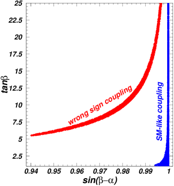
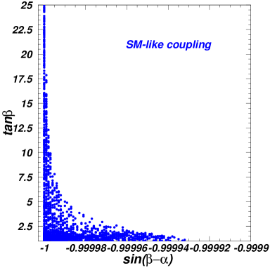
where denotes or . In the type-II 2HDM, the 125 GeV Higgs is allowed to have the SM-like coupling and wrong sign Yukawa coupling,
| (8) |
III The experimental constraints of the Higgs data at the LHC
III.1 Numerical calculations
We take the light CP-even Higgs boson as the SM-like Higgs, GeV. The measurement of the branching fraction of gives the stringent constraints on the charged Higgs mass of the type-II 2HDM, GeV bsr570 . If the 125 GeV Higgs boson is the portal between the DM and SM sectors, it is favored to have wrong sign Yukawa coupling which can realize the isospin-violating DM interactions with nucleons and relax the bounds of direct detection of DM. However, Ref. PT_2HDM2 shows the the wrong sign Yukwa coupling region of type-II 2HDM is strongly restricted by the requirement of SFOEWPT. Therefore, in this paper we take the heavy CP-even Higgs as the only portal between the DM and SM sectors, and focus on the case of the 125 GeV with the SM-like couping. The , , and oblique parameters give the stringent constraints on the mass spectrum of Higgses of type-II 2HDM 1604.01406 ; 1701.02678 ; 2003.06170 . One of and is around 600 GeV, and another is allowed to have a wide mass range including low mass 1701.02678 ; 2003.06170 . Therefore, we fix GeV to make the portal to have a wide mass range.
In our calculation, we consider the following observables and constraints:
-
(1)
Theoretical constraints. The scalar potential of the model contains one of the type-II 2HDM and one of the DM sector. The vacuum stability, perturbativity, and tree-level unitarity impose constraints on the relevant parameters, which are discussed in detail in Refs. 2hisos-4 ; 2hisos-6 . Here we employ the formulas in 2hisos-4 ; 2hisos-6 to implement the theoretical constraints. Compared to Refs. 2hisos-4 ; 2hisos-6 , there are additional factors of in the term and the term of this paper. In addition, we require that the potential has a global minimum at the point of (, , ).
- (2)
-
(3)
The flavor observables and . We employ SuperIso-3.4 spriso to calculate , and is calculated following the formulas in deltmq . Besides, we include the constraints of bottom quarks produced in decays, , which is calculated following the formulas in rb1 ; rb2 .
Channel Experiment Mass range [GeV] Luminosity ATLAS 8 TeV 47Aad:2014vgg 90-1000 19.5-20.3 fb-1 CMS 8 TeV 48CMS:2015mca 90-1000 19.7 fb-1 CMS 13 TeV add-hig-16-037 90-3200 12.9 fb-1 CMS 13 TeV 1709.07242 200-2250 36.1 fb-1 CMS 8 TeV 1511.03610 25-80 19.7 fb-1 ATLAS 13 TeV 2002.12223 200-2500 139 fb-1 CMS 8 TeV CMS-HIG-15-009 25-60 19.7 fb-1 ATLAS 13 TeV 80lenzi 200-2400 15.4 fb-1 CMS 8+13 TeV 81rovelli 500-4000 12.9 fb-1 + CMS 8 TeV HIG-17-013-pas 80-110 19.7 fb-1 + CMS 13 TeV HIG-17-013-pas 70-110 35.9 fb-1 + CMS 8 TeV HIG-17-013-pas 80-110 19.7 fb-1 + CMS 13 TeV HIG-17-013-pas 70-110 35.9 fb-1 ATLAS 8 TeV 55Aad:2015agg 300-1500 20.3 fb-1 ATLAS 13 TeV 77atlasww13 300-3000 13.2 fb-1 ATLAS 13 TeV 78atlasww13lvqq 500-3000 13.2 fb-1 ATLAS 13 TeV 1710.07235 200-3000 36.1 fb-1 ATLAS 13 TeV 1710.01123 200-3000 36.1 fb-1 CMS 13 TeV 1912.01594 200-3000 35.9 fb-1 ATLAS 8 TeV 57Aad:2015kna 160-1000 20.3 fb-1 ATLAS 13 TeV 74koeneke4 300-1000 13.3 fb-1 ATLAS 13 TeV 75koeneke5 300-3000 13.2 fb-1 ATLAS 13 TeV 75koeneke5 300-3000 13.2 fb-1 ATLAS 13 TeV 76koeneke3 200-3000 14.8 fb-1 ATLAS 13 TeV 1712.06386 200-2000 36.1 fb-1 ATLAS 13 TeV 1708.09638 300-5000 36.1 fb-1 Table 1: The upper limits at 95% C.L. on the production cross-section times branching ratio of , , , , and considered in the and searches at the LHC. Channel Experiment Mass range [GeV] Luminosity CMS 8 TeV 64Khachatryan:2016sey 250-1100 19.7 fb-1 CMS 8 TeV 65Khachatryan:2015yea 270-1100 17.9 fb-1 CMS 8 TeV 66Khachatryan:2015tha 260-350 19.7 fb-1 ATLAS 13 TeV 84varol 300-3000 13.3 fb-1 CMS 13 TeV 1710.04960 750-3000 35.9 fb-1 CMS 13 TeV 1707.02909 250-900 35.9 fb-1 CMS 13 TeV 1811.09689 250-3000 35.9 fb-1 CMS 13 TeV 2006.06391 260-1000 35.9 fb-1 CMS 13 TeV 2007.14811 1000-3000 139 fb-1 CMS 8 TeV 66Khachatryan:2015tha 220-350 19.7 fb-1 CMS 8 TeV 67Khachatryan:2015lba 225-600 19.7 fb-1 ATLAS 8 TeV 68Aad:2015wra 220-1000 20.3 fb-1 ATLAS 8 TeV 68Aad:2015wra 220-1000 20.3 fb-1 ATLAS 13 TeV 1712.06518 200-2000 36.1 fb-1 CMS 13 TeV 1903.00941 225-1000 35.9 fb-1 CMS 13 TeV 1910.11634 220-400 35.9 fb-1 ATLAS 8 TeV 1505.01609 4-50 20.3 fb-1 CMS 8 TeV 1701.02032 5-15 19.7 fb-1 CMS 8 TeV 1701.02032 25-62.5 19.7 fb-1 CMS 8 TeV 1701.02032 15-62.5 19.7 fb-1 CMS 13 TeV 1805.10191 15-60 35.9 fb-1 CMS 13 TeV 1907.07235 4-15 35.9 fb-1 CMS 13 TeV 2005.08694 3.6-21 35.9 fb-1 CMS 8 TeV 160302991 40-1000 19.8 fb-1 CMS 8 TeV 160302991 20-1000 19.8 fb-1 ATLAS 13 TeV 1804.01126 130-800 36.1 fb-1 CMS 13 TeV 1911.03781 30-1000 35.9 fb-1 Table 2: The upper limits at 95% C.L. on the production cross-section times branching ratio for the channels of Higgs-pair and a Higgs production in association with at the LHC. -
(4)
The global fit to the 125 GeV Higgs signal data. The version 2.0 of Lilith lilith is used to perform the calculation for the signal strengths of the 125 GeV Higgs combining the LHC run-I and run-II data (up to datasets of 36 fb-1). We pay particular attention to the surviving samples with , where denotes the minimum of . These samples correspond to be within the range in any two-dimension plane of the model parameters when explaining the Higgs data.
-
(5)
The exclusion limits of searches for additional Higgs bosons. We use HiggsBounds-4.3.1 hb1 ; hb2 to implement the exclusion constraints from the neutral and charged Higgs searches at LEP at 95% confidence level.
Because the -quark loop and top quark loop have destructive interference contributions to production in the type-II 2HDM, the cross section decreases with an increase of , reaches the minimum value for the moderate , and is dominated by the -quark loop for enough large . In addition to and , the cross section of depends on . We employ SusHi to compute the cross sections for and in the gluon fusion and -associated production at NNLO in QCD sushi . The cross sections of via vector boson fusion process are deduced from results of the LHC Higgs Cross Section Working Group higgswg . We employ 2HDMC to calculate the branching ratios of the various decay modes of and . The searches for the additional Higgs considered by us are listed in Tables 1 and 2. The LHC searches for can not impose any constraints on the model for GeV and 1 mhp500 . Therefore, we do not consider the constraints from the searches for the heavy charged Higgs.
III.2 Results and discussions
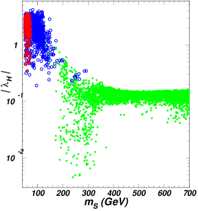
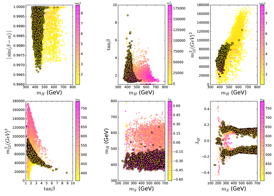
In Fig. 1, we show and allowed by the 125 GeV Higgs signal data at the LHC. From Fig. 1, we see that and have strong correlation due to the constraints of the 125 GeV Higgs data, especially for the case of the wrong sign Yukawa coupling. The wrong sign Yukawa coupling can be achieved only for , and is restricted to be in a very narrow range for a given . For the case of the SM-like coupling, is required to be in two very narrow ranges of and . The is allowed to be as low as 1.0, and its upper bound increases with in the case of the the SM-like Higgs coupling.
Now we examine the parameter space of 2HDMIID using the exclusion limits of searches for additional Higgses at the LHC. In the 2HDMIID, we take the heavy CP-even Higgs as only portal between DM and SM sectors, and the decay opens for . The decay mode possibly affects the allowed parameter space, but the constraints of the DM observables have to be simultaneously considered. Here we temporarily assume , and close the decay mode. In the next section, the effects of will be considered by combining the DM observables.
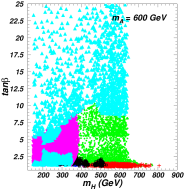
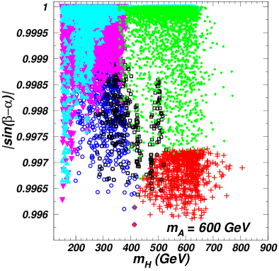
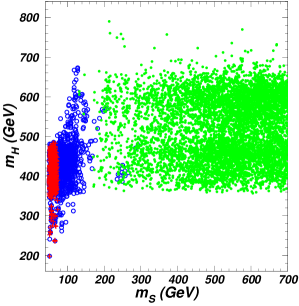
In Fig. 2, we project the surviving samples with the SM-like coupling on the planes of versus and versus after imposing the constraints of pre-LHC (denoting theoretical constraints, electroweak precision data, the flavor observables, , the exclusion limits from searches for Higgs at LEP), the 125 GeV Higgs signal data, and the searches for additional Higgses at the LHC. Note that in the region of , the signal data of the 125 GeV Higgs require to nearly equal to -1.0, as shown in right panel of Fig. 1. For such case, the couplings of and are almost the same as those in the case of . Therefore, we do not distinguish the sign of when discussing the constraints on and from the LHC direct searches.
From Fig. 2, we find the joint constraints of , , , and exclude the whole region of GeV. The channels impose upper bound on in the whole range of , and allow to vary from 150 GeV to 800 GeV for appropriate values of and . The channel does not constrain the parameter space of 360 GeV since the branching ratio of rapidly decreases with an increase of . The limits of channel can be relaxed by a small which suppresses the coupling.
The and channels impose strong constraints on the regions with small values of and since the couplings of and increase with decreasing of , and is enhanced by the top quark loop for a small . In addition, the Fig. 1 shows that the 125 GeV Higgs signal data favor a small for a small in the case of the SM-like coupling. With an increase of , the channel opens and enhances the total width of sizably, so that the constraints from channels are relaxed. Different from other channels, the channel gives the constraints on the region with a large . This is because the width of decreases with an increase of , and thus increases with .
IV The dark matter observables
We use FeynRules feyrule to generate the model file, which is called by micrOMEGAs micomega to calculate the relic density. In our scenario, the elastic scattering of on a nucleon receives the contributions of the process with -channel exchange of , and the spin-independent cross section between DM and nucleons is given by sigis
| (11) |
where ,
| (12) |
with . The values of the form factors and are extracted from micrOMEGAs micomega .
The Planck collaboration reported the relic density of cold DM in the universe, planck . The XENON1T collaboration reported stringent upper bounds of the spin-independent DM-nucleon cross section xenon2018 . The Fermi-LAT searches for the DM annihilation from dwarf spheroidal satellite galaxies gave the upper limits on the averaged cross sections of the DM annihilation to , , , , , and fermi .
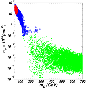
In Fig. 3, we project the surviving samples on the planes of versus , versus , and versus after imposing the constraints of ”pre-LHC”, the Higgs data at the LHC, the relic density, XENON1T, and Fermi-LAT. The middle panel shows that the decay weakens the constraints of the LHC Higgs data compared to Fig.2. For example, is allowed to be as low as 200 GeV for a light DM. However, the upper bounds of the XENON1T and Fermi-LAT exclude GeV and 360 GeV. In order to obtain the correct relic density, is favored to increase with decreasing of . Thus, for a small , a large can enhance the spin-independent DM-nucleon cross section and the averaged cross sections of the today DM annihilation to the SM particles, leading that GeV and 75 GeV are respectively excluded by the experimental data of the XENON1T and Fermi-LAT. For 180 GeV 340 GeV, can be allowed to be smaller than 0.01 because of the resonant contribution at .
V Electroweak phase transition and gravitational wave
The phase transition can proceed in basically two different ways. In a first-order phase transition, at the critical temperature , the two degenerate minima will be at different points in field space, typically with a potential barrier in between. For a second order (cross-over) transition, the broken and symmetric minimum are not degenerate until they are at the same point in field space. In this paper we focus on the SFOEWPT, which is required by a successful explanation of the observed BAU and can produce primordial GW signals.
V.1 The thermal effective potential
In order to examine electroweak phase transition (EWPT), we first take , , and as the field configurations, and obtain the field dependent masses of the scalars (), the Goldstone boson (), the gauge boson, and fermions. The masses of scalars are given
| (13) | ||||
| (14) | ||||
| (15) |
| (16) |
where , , and .
The masses of gauge boson are given
| (17) |
We neglect the contributions of light fermions, and only consider the masses of top quark and bottom quark,
| (18) |
where and
Now we study the effective potential with thermal correction. The thermal effective potential in terms of the classical fields () is composed of four parts:
| (19) |
Where is the tree-level potential, is the Coleman-Weinberg potential, is the counter term, is the thermal correction, and is the resummed daisy corrections. In this paper, we calculate in the Landau gauge.
We obtain the tree-level potential in terms of their classical fields ()
| (20) | |||||
The Coleman-Weinberg potential in the scheme at 1-loop level has the form Coleman:1973jx :
| (21) |
where , and is the spin of particle i. is a renormalization scale, and we take . The constants for scalars or fermions and for gauge bosons. is the number of degree of freedom,
| (22) |
With being included in the potential, the minimization conditions of scalar potential in Eq. (19) and the CP-even mass matrix will be shifted slightly. To maintain the minimization conditions at T=0, we add the so-called “counter-terms”
| (23) |
where the relevant coefficients are determined by
| (24) |
| (25) |
which are evaluated at the EW minimum of on both sides. As a result, the VEVs of , , and the CP-even mass matrix will not be shifted.
It is a well-known problem that the second derivative of the Coleman-Weinberg potential at suffers from logarithmic divergences originating from the vanishing Goldstone masses. To solve the divergence problem, we take a straightforward approach of imposing an IR cut-off at for the masses of Goldstone boson of the divergent terms, which gives a good approximation to the exact procedure of on-shell renormalization, as argued in PT_2HDM1.5 .
The thermal contributions to the potential can be written as v1t
| (26) |
where , and the functions are
| (27) |
Finally, the thermal corrections with resumed ring diagrams are given vdai1 ; vdai2
| (28) |
where . The , and are the longitudinal gauge bosons with . The thermal Debye masses are the eigenvalues of the full mass matrix,
| (29) |
where . are given by
| (30) |
The physical mass of the longitudinally polarized boson is
| (31) |
The physical mass of the longitudinally polarized and boson
| (32) |
with
| (33) |
V.2 Calculation of electroweak phase transition and gravitational wave
In a first-order cosmological phase transition, bubbles nucleate and expand, converting the high-temperature phase into the low-temperature one. The bubble nucleation rate per unit volume at finite temperature is given by bubble-0 ; bubble-1 ; bubble-2
| (34) |
where is a prefactor and is the Euclidean action
| (35) |
At the nucleation temperature , the thermal tunneling probability for bubble nucleation per horizon volume and per horizon time is of order one, and the conventional condition is . The bubbles nucleated within one Hubble patch proceed to expand and collide, until the entire volume is filled with the true vacuum.
There are two key parameters characterizing the dynamics of the EWPT, and . describes roughly the inverse time duration of the strong first order phase transition,
| (36) |
where is the Hubble parameter at the bubble nucleation temperature . is defined as the vacuum energy released from the phase transition normalized by the total radiation energy density at ,
| (37) |
where is the effective number of relativistic degrees of freedom. We use the numerical package CosmoTransitions cosmopt and PhaseTracer Athron:2020sbe to analyze the phase transition and computes quantities related to cosmological phase transition.
In a radiation-dominated Universe, there are three sources of GW production at a EWPT: bubble collisions, in which the localized energy density generates a quadrupole contribution to the stress-energy tensor, which in turn gives rise to GW, plus sound waves in the plasma and magnetohydrodynamic (MHD) turbulence. The total resultant energy density spectrum can be approximately given as,
| (38) |
Recent studies show that the energy deposited in the bubble walls is negligible, despite the possibility that the bubble walls can run away in some circumstances gw-coll-1 . Therefore, although a bubble wall can reach relativistic speed, its contribution to GW can generally be neglected gw-coll-2 ; gw-coll-3 . Therefore, in the following discussions we do not include the contribution from bubble collision .
The GW spectrum from the the sound waves can be obtained by fitting to the result of numerical simulations gw-sw ,
| (39) | |||||
where is the present peak frequency of the spectrum,
| (40) |
is the wall velocity, and the factor is the fraction of latent heat transformed into the kinetic energy of the fluid. and are difficult to compute, and involves certain assumptions regarding the dynamics of the bubble walls. On the other hand, successful electroweak baryogenesis scenarios favor lower wall velocity ewbg-vw , which allows the effective diffuse of particle asymmetries near the bubble wall front. In Ref. new-ewbg-vw , however, it is pointed out that the relevant velocity for electroweak baryogenesis is not really , but the relative velocity between the bubble wall and the plasma in the deflagration front. As a result, the electroweak baryogenesis is not necessarily impossible even in the case with large . Therefore, in this paper we take two different cases of and 1004.4187 :
-
•
For small wall velocity: and
(41) -
•
For very large wall velocity: and
(42)
Considering Kolmogorov-type turbulence as proposed in Ref. mhd-type , the GW spectrum from the MHD turbulence has the form mhd-1 ; mhd-2 ,
| (43) | |||||
with the red-shifted Hubble rate at GW generation
| (44) |
The peak frequency is given by
| (45) |
The energy fraction transferred to the MHD turbulence can vary between to of gw-sw . Here we take .
V.3 Results and discussions
The strength of the electroweak phase transition is quantified as
| (46) |
with at critical temperature . The global minimum of potential has because of the CP-conserving case. In order to avoid washing out the baryon number generated during the phase transition, a SFOEWPT is required and the conventional condition is .
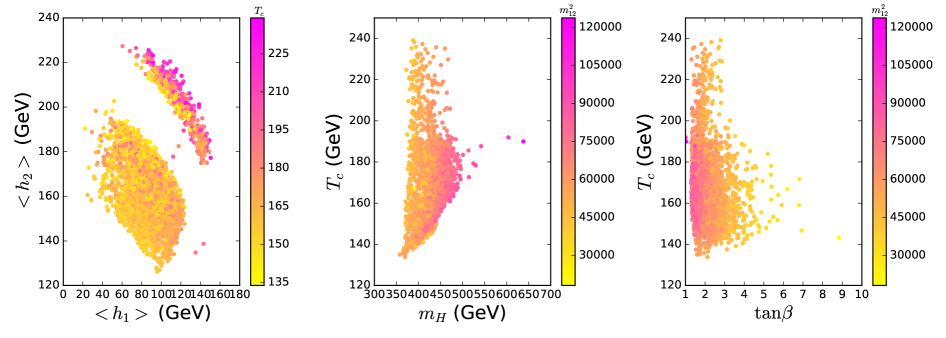
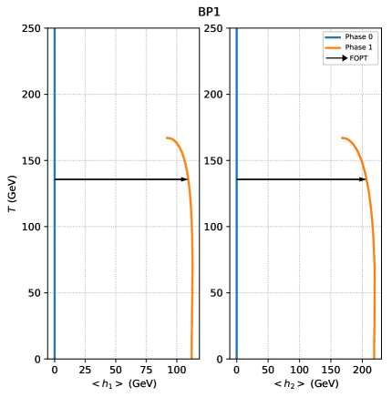
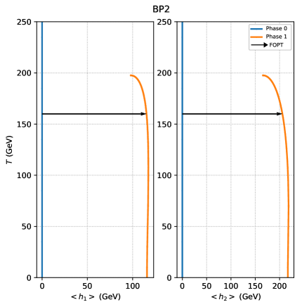
After imposing the constraints of ”pre-LHC”, the LHC Higgs data, the relic density, XENON1T, and Fermi-LAT, we scan over the parameter space in the previous selected scenario. We find some surviving samples which can achieve a SFOEWPT, and these samples are projected in Fig. 4 and Fig. 5. For all the surviving samples, at the two degenerate minima of potential are respectively at () and (0, 0, 0). In the process of EWPT, always has no VEV.
From Fig. 4, we find that and can vary in the ranges of 20 GeV 150 GeV and 125 GeV 230 GeV with varying from 134 GeV to 240 GeV. tends to increase with , and has a relative small value for a large . It should also be noted that the relic abundance of the DM is achieved by the thermal freeze-out in the early universe when the temperature was about . In the model, is much larger than for 50 GeV GeV. Therefore, the EWPT hardly affects the thermal freeze-out process of DM.
From Fig. 5 , we find that a SFOEWPT favors a small , namely a large mass splitting between and , which is consistent with Refs. PT_2HDM2 ; PT_2HDM3 . Most of samples lie in the region of GeV, and there are several samples with 500 GeV when is very closed to 1.0. Also a SFOEWPT favors to increase with and decrease with an increase of . There is a relative strong correlation between and , and is imposed upper and lower bounds for a given . With an increase of , is stringently restricted by the theoretical constraints and the LHC Higgs data, leading that it is difficult to achieve a SFOEWPT. Thus, most of samples lie in the region of small . The requirement of a SFOEWPT is not sensitive to , and disfavors 0.3.
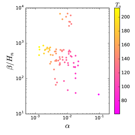
Now we examine two key parameters and which characterize the dynamics of the SFOEWPT, and govern the strength of GW spectra. A larger and smaller can lead to stronger GW signals. In addition to the conditions of the successful bubble nucleations, we require
| (47) |
with at the nucleation temperature . In fact, this is a more precise condition of SFOEWPT than . Also note that there generically exists a difficulty for solving bounce solution in a very thin-walled bubble, including the package CosmoTransitions BubbleProfiler . Therefore, we will neglect the samples with very thin-walled bubble. Consider the constraints discussed above, we find some surviving samples, and the corresponding and are shown in Fig. 6.
| BP1 | BP2 | |
|---|---|---|
| 0.9998 | 0.9991 | |
| 1.95 | 1.87 | |
| (GeV) | 369.55 | 387.97 |
| (GeV) | 620.8 | 618.31 |
| (GeV | 53049.1 | 53649.1 |
| (GeV) | 479.2 | 501.7 |
| 0.133 | -0.129 | |
| 12.3 | 10.93 | |
| (GeV) | 135.7 | 160.0 |
| (GeV) | 61.0 | 95.0 |
| 35.6 | 102.8 | |
| 0.094 | 0.018 |
The may characterize the inverse time duration of the EWPT. A small means a long EWPT, and gives strong GW signals. For the GW coming from the sound waves in the plasma, the GW signal will continue being generated and the energy density of the GW is thus proportional to the duration of the EWPT if the mean square fluid velocity of the plasma is non-negligible gw-sw . In addition, a large can enhance the peak frequency of the GW spectra. The parameter describes the amount of energy released during the EWPT, and therefore a large leads to strong GW signals.
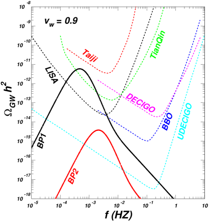
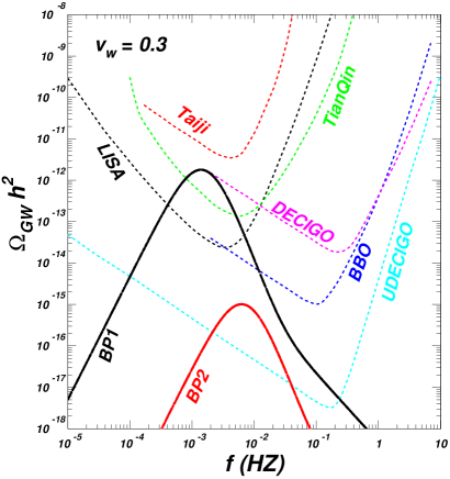
We pick out two benchmark points (BPs), and examine the corresponding GW spectra. Table 3 shows the input and output parameters of the BPs. Their phase histories are exhibited in Fig. 7 on filed configurations versus temperature plane. The filed configuration is not shown as the minima at any temperatures locate at . In Fig. 8, we show predicted GW spectra for our BPs along with expected sensitivities of various future interferometer experiments, and find that the amplitudes of the GW spectra reach the sensitivities of LISA, TianQin, BBO, DECIGO, UDECIGO for BP1 (UDECIGO for BP2).
VI Conclusion
We examine the status of the 2HDMIID confronted with the recent LHC Higgs data, the DM observables and SFOEWPT, and discuss the detectability of GW at the future GW detectors. We choose the heavy CP-even Higgs as the only portal between the DM and SM sectors, and focus on the case of the 125 GeV Higgs with the SM-like coupling. We find that for GeV, 130 GeV and 360 GeV are excluded by the joint constraints of the 125 GeV Higgs signal data, the searches for additional Higgs via , , at the LHC as well as the relic density, XENON1T.
A SFOEWPT can be achieved in the many regions of GeV and GeV, favors a small , and is not sensitive to the mass of DM. We find the benchmark points for which the predicted GW spectra can reach the sensitivities of LISA, TianQin, BBO, DECIGO, and UDECIGO.
Acknowledgment
We thank L. Bian, Wei Chao and Huai-Ke Guo for helpful discussions. This work was supported by the National Natural Science Foundation of China under grant 11975013, by the Natural Science Foundation of Shandong province (ZR2017MA004 and ZR2017JL002), and by the ARC Centre of Excellence for Particle Physics at the Tera-scale under the grant CE110001004. This work is also supported by the Project of Shandong Province Higher Educational Science and Technology Program under Grants No. 2019KJJ007.
References
- (1) T. D. Lee, Phys. Rev. D 8, 1226 (1973).
- (2) H. E. Haber, G. L. Kane and T. Sterling, Nucl. Phys. B 161, 493 (1979).
- (3) J. F. Donoghue and L. F. Li, Phys. Rev. D 19, 945 (1979).
- (4) X.-G. He, T. Li, X.-Q. Li, J. Tandean, H.-C. Tsai, Phys. Rev. D 79, 023521 (2009).
- (5) X.-G. He, J. Tandean, Phys. Rev. D 88, 013020 (2013).
- (6) Y. Cai, T. Li, Phys. Rev. D 88, 115004 (2013).
- (7) L. Wang, X.-F. Han, Phys. Lett. B 739, 416-420 (2014).
- (8) A. Drozd, B. Grzadkowski, J. F. Gunion, Y. Jiang, JHEP 1411, 105 (2014).
- (9) X.-G. He, J. Tandean, JHEP 1612, 074 (2016).
- (10) T. Alanne, K. Kainulainen, K. Tuominen, V. Vaskonen, JCAP 1608, 057 (2016).
- (11) L. Wang, R. Shi, X.-F. Han, Phys. Rev. D 96, 115025 (2017).
- (12) N. Chen, Z. Kang, J. Li, Phys. Rev. D 95, 015003 (2017).
- (13) L. Wang, X.-F. Han, B. Zhu, Phys. Rev. D 98, 035024 (2018).
- (14) S. Baum, N. R. Shah, JHEP 12, 044 (2018).
- (15) A. I. Bochkarev, S. V. Kuzmin and M. E. Shaposhnikov, Phys. Lett. B 244, 275 (1990); J. M. Cline, P.-A. Lemieux, Phys. Rev. D 55, 3873 (1997); G. C. Dorsch, S. J. Huber and J. M. No, JHEP 1310, 029 (2013); G. C. Dorsch, S. J. Huber, K. Mimasu and J. M. No, Phys. Rev. Lett. 113, 211802 (2014); N. Chen, T. Li, Z. Teng, Y. Wu, arXiv:2006.06913; R. Zhou, L. Bian, arXiv:2001.01237; R. Zhou, L. Bian, H.-K Guo, Phys. Rev. D 101, 091903 (2020); X. Wang, F. Huang, X. Zhang, Phys. Rev. D 101, 015015 (2020); JCAP 05, 045 (2020).
- (16) J. M. Cline, K. Kainulainen and M. Trott, JHEP 1111, 089 (2011).
- (17) P. Basler, M. Krause, M. Muhlleitner, J. Wittbrodt and A. Wlotzka, JHEP 1702, 121 (2017).
- (18) J. Bernon, L. Bian and Y. Jiang, JHEP 1805, 151 (2018).
- (19) A. D. Sakharov, Pisma Zh. Eksp. Teor. Fiz. 5, 32 (1967) [JETP Lett. 5, 24 (1967)] [Sov. Phys. Usp. 34, no. 5, 392 (1991)] [Usp. Fiz. Nauk 161, no. 5, 61 (1991)].
- (20) M. Kamionkowski, A. Kosowsky and M. S. Turner, Phys. Rev. D 49, 2837 (1994).
- (21) LISA Collaboration, H. Audley et al., “Laser Interferometer Space Antenna,” arXiv:1702.00786.
- (22) X. Gong et al., “Descope of the ALIA mission,” J. Phys. Conf. Ser. 610, 012011 (2015).
- (23) TianQin Collaboration, J. Luo et al., “TianQin: a space-borne gravitational wave detector,” Class. Quant. Grav. 33, 035010 (2016).
- (24) K. Yagi and N. Seto, “Detector configuration of DECIGO/BBO and identification of cosmological neutron-star binaries,” Phys. Rev. D 83, 044011 (2011).
- (25) H. Kudoh, A. Taruya, T. Hiramatsu, and Y. Himemoto, “Detecting a gravitational-wave background with next-generation space interferometers,” Phys. Rev. D 73, 064006 (2006).
- (26) R. A. Battye, G. D. Brawn, A. Pilaftsis, JHEP 1108, 020 (2011).
- (27) Heavy Flavor Averaging Group, Eur. Phys. Jour. C 77, 895 (2017); M. Misiak, M. Steinhauser, Eur. Phys. Jour. C 77, 201 (2017).
- (28) F. Kling, J. M. No, S. Su, JHEP 1609, 093 (2016).
- (29) L. Wang, F. Zhang, X.-F. Han, Phys. Rev. D 95, 115014 (2017).
- (30) L. Wang, H.-X. Wang, X.-F. Han, Comput. Phys. Commun. 44, 073101 (2020).
- (31) D. Eriksson, J. Rathsman, O. Stål, Comput. Phys. Commun. 181, 189 (2010).
- (32) M. Tanabashi et al., [Particle Data Group], Phys. Rev. D 98, 030001 (2018).
- (33) F. Mahmoudi, Comput. Phys. Commun. 180, 1579-1673 (2009).
- (34) C. Q. Geng and J. N. Ng, Phys. Rev. D 38, 2857 (1988) [Erratum-ibid. D 41, 1715 (1990)].
- (35) H. E. Haber, H. E. Logan, Phys. Rev. D 62, 015011 (2010).
- (36) G. Degrassi, P. Slavich, Phys. Rev. D 81, 075001 (2010).
- (37) J. Bernon, B. Dumont, S. Kraml, Phys. Rev. D 90, 071301 (2014); S. Kraml, T. Q. Loc, D. T Nhung, L. D. Ninh, arXiv:1908.03952.
- (38) P. Bechtle, O. Brein, S. Heinemeyer, G. Weiglein, K. E. Williams, Comput. Phys. Commun. 181, 138-167 (2010).
- (39) P. Bechtle, O. Brein, S. Heinemeyer, O. Stål, T. Stefaniak, G. Weiglein, K. E. Williams, Eur. Phys. Jour. C 74, 2693 (2014).
- (40) R. V. Harlander, S. Liebler, H. Mantler, Comput. Phys. Commun. 184, 1605 (2013).
- (41) S. Heinemeyer et al. [LHC Higgs Cross Section Working Group Collaboration], arXiv:1307.1347.
- (42) S. Moretti, arXiv:1612.02063.
- (43) ATLAS Collaboration, G. Aad et al., “Search for neutral Higgs bosons of the minimal supersymmetric standard model in pp collisions at = 8 TeV with the ATLAS detector,” JHEP 11, 056 (2014).
- (44) CMS Collaboration, “Search for additional neutral Higgs bosons decaying to a pair of tau leptons in collisions at = 7 and 8 TeV,” CMS-PAS-HIG-14-029.
- (45) CMS Collaboration, “Search for a neutral MSSM Higgs Boson decaying into with 12.9 fb-1 of data at = 13 TeV,” CMS-PAS-HIG-16-037.
- (46) ATLAS Collaboration, “Search for additional heavy neutral Higgs and gauge bosons in the ditau final state produced in 36 fb-1 of pp collisions at = 13 TeV with the ATLAS detector,” JHEP 1801, 055 (2018).
- (47) CMS Collaboration, “Search for a low-mass pseudoscalar Higgs boson produced in association with a pair in pp collisions at = 8 TeV,” Phys. Lett. B 758, 296-320 (2016).
- (48) ATLAS Collaboration, “Search for heavy Higgs bosons decaying into two tau leptons with the ATLAS detector using p p collisions at at = 13 TeV,” arXiv:2002.12223.
- (49) CMS Collaboration, “Search for a light pseudoscalar Higgs boson produced in association with bottom quarks in pp collisions at = 8 TeV,” CMS-HIG-15-009.
- (50) ATLAS Collaboration, “Search for scalar diphoton resonances with 15.4 fb-1 of data collected at =13 TeV in 2015 and 2016 with the ATLAS detector,” ATLAS-CONF-2016-059.
- (51) CMS Collaboration, “Search for resonant production of high mass photon pairs using of proton-proton collisions at and combined interpretation of searches at 8 and 13 TeV,” CMS-PAS-EXO-16-027.
- (52) CMS Collaboration, “Search for new resonances in the diphoton final state in the mass range between 70 and 110 GeV in pp collisions at = 8 and 13 TeV,” CMS-PAS-HIG-17-013.
- (53) ATLAS Collaboration, G. Aad et al., “Search for a high-mass Higgs boson decaying to a boson pair in collisions at TeV with the ATLAS detector,” JHEP 01, (2016) 032.
- (54) ATLAS collaboration, “Search for a high-mass Higgs boson decaying to a pair of W bosons in pp collisions at TeV with the ATLAS detector,” ATLAS-CONF-2016-074.
- (55) ATLAS Collaboration, “Search for diboson resonance production in the final state using p p collisions at = 13 TeV with the ATLAS detector at the LHC,” ATLAS-CONF-2016-062.
- (56) ATLAS Collaboration, “Search for WW/WZ resonance production in final states in pp collisions at = 13 TeV with the ATLAS detector,” arXiv:1710.07235.
- (57) ATLAS Collaboration, “Search for heavy resonances decaying into WW in the final state in pp collisions = 13 TeV with the ATLAS detector,” Eur. Phys. Jour. C 78, 24 (2018).
- (58) CMS Collaboration, “Search for a heavy Higgs boson decaying to a pair of W bosons in proton-proton collisions at = 13 TeV,” arXiv:1912.01594.
- (59) ATLAS Collaboration, G. Aad et al., “Search for an additional, heavy Higgs boson in the decay channel at in collision data with the ATLAS detector,” Eur. Phys. Jour. C 76, 45 (2016).
- (60) ATLAS Collaboration, “Search for new phenomena in the final state at = 13 TeV with thee ATLAS detector,” ATLAS-CONF-2016-056.
- (61) ATLAS Collaboration, “Searches for heavy ZZ and ZW resonances in the and vvqq final states in pp collisions at TeV with the ATLAS detector,” ATLAS-CONF-2016-082.
- (62) ATLAS Collaboration, “Study of the Higgs boson properties and search for high-mass scalar resonances in the decay channel at = 13 TeV with the ATLAS detector,” ATLAS-CONF-2016-079.
- (63) ATLAS Collaboration, “Search for heavy ZZ resonances in the and final states using proton proton collisions at = 13 TeV with the ATLAS detector,” arXiv:1712.06386.
- (64) ATLAS Collaboration, “Searches for heavy ZZ and ZW resonances in the and final states in pp collisions at = 13 TeV with the ATLAS detector,” arXiv:1708.09638.
- (65) CMS Collaboration, V. Khachatryan et al., “Search for two Higgs bosons in final states containing two photons and two bottom quarks,” Phys. Rev. D 94, 052012 (2016).
- (66) CMS Collaboration, V. Khachatryan et al., “Search for resonant pair production of Higgs bosons decaying to two bottom quark–antiquark pairs in proton–proton collisions at 8 TeV,” Phys. Lett. B 749, 560-582 (2015).
- (67) CMS Collaboration, V. Khachatryan et al., “Searches for a heavy scalar boson H decaying to a pair of 125 GeV Higgs bosons hh or for a heavy pseudoscalar boson A decaying to Zh, in the final states with ,” Phys. Lett. B 755, 217-244 (2016).
- (68) ATLAS Collaboration, “Search for pair production of Higgs bosons in the final state using protonproton collisions at TeV with the ATLAS detector,” ATLAS-CONF-2016-049.
- (69) CMS Collaboration, “Search for a massive resonance decaying to a pair of Higgs bosons in the four b quark final state in proton-proton collisions at TeV,” arXiv:1710.04960.
- (70) CMS Collaboration, “Search for Higgs boson pair production in events with two bottom quarks and two tau leptons in proton-proton collisions at TeV,” arXiv:1707.02909.
- (71) CMS Collaboration, “Combination of searches for Higgs boson pair production in proton-proton collisions at at TeV,” Phys. Rev. Lett. 122, 121803 (2019).
- (72) CMS Collaboration, “Search for resonant pair production of Higgs bosons in the channel in proton-proton collisions at TeV,” arXiv:2006.06391.
- (73) ATLAS Collaboration, “Reconstruction and identification of boosted di- systems in a search for Higgs boson pairs using 13 TeV proton–proton collision data in ATLAS,” arXiv:2007.14811.
- (74) CMS Collaboration, V. Khachatryan et al., “Search for a pseudoscalar boson decaying into a boson and the 125 GeV Higgs boson in final states,” Phys. Lett. B 748, 221-243 (2015).
- (75) ATLAS Collaboration, G. Aad et al., “Search for a CP-odd Higgs boson decaying to Zh in pp collisions at TeV with the ATLAS detector,” Phys. Lett. B 744, 163-183 (2015).
- (76) ATLAS Collaboration, “Search for heavy resonances decaying into a W or Z boson and a Higgs boson in final states with leptons and b-jets in 36 of = 13 pp collisions with the ATLAS detector,” arXiv:1712.06518.
- (77) CMS Collaboration, “Search for a heavy pseudoscalar boson decaying to a Z and a Higgs boson at = 13 TeV,” Eur. Phys. Jour. C 79, 564 (2019).
- (78) CMS Collaboration, “Search for a heavy pseudoscalar Higgs boson decaying into a 125 GeV Higgs boson and a boson in final states with two tau and two light leptons at = 13 TeV,” arXiv:1910.11634.
- (79) ATLAS Collaboration, “Search for Higgs bosons decaying to aa in the final state in pp collisions at = 8 TeV with the ATLAS experiment,” Phys. Rev. D 92, 052002 (2015).
- (80) CMS Collaboration, “Search for light bosons in decays of the 125 GeV Higgs boson in proton-proton collisions at = 8 TeV,” JHEP 1710, 076 (2017).
- (81) CMS Collaboration, “Search for an exotic decay of the Higgs boson to a pair of light pseudoscalars in the final state with two quarks and two leptons in proton-proton collisions at = 13 TeV,” Phys. Lett. B 785, 462 (2018).
- (82) CMS Collaboration, “Search for light pseudoscalar boson pairs produced from decays of the 125 GeV Higgs boson in final states with two muons and two nearby tracks in pp collisions at = 13 TeV,” arXiv:1907.07235.
- (83) CMS Collaboration, “Search for a light pseudoscalar Higgs boson in the boosted final state in proton-proton collisions at = 13 TeV,” arXiv:2005.08694.
- (84) CMS Collaboration, V. Khachatryan et al., “Search for neutral resonances decaying into a Z boson and a pair of b jets or leptons,” Phys. Lett. B 759, 369-394 (2016).
- (85) ATLAS Collaboration, “Search for a heavy Higgs boson decaying into a Z boson and another heavy Higgs boson in the bb final state in p p collisions =13 TeV with the ATLAS detector,” Phys. Lett. B 783, 392 (2018).
- (86) CMS Collaboration, “Search for new neutral Higgs bosons through the process in pp collisions at =13 TeV,” arXiv:1911.03781.
- (87) A. Alloul et al., Comput. Phys. Commun. 185, 2250 (2014).
- (88) G. Belanger, F. Boudjema, A. Pukhov, A. Semenov, Comput. Phys. Commun. 185, 960-985 (2014).
- (89) G. Jungman, M. Kamionkowski, K. Griest, Phys. Rept. 267, 195 (1996); M. A. Shifman, A. I. Vainshtein, V. I. Zakharov, Phys. Lett. B 78, 443 (1978).
- (90) Planck Collaboration, Astron. Astrophys. A 27, 594 (2016).
- (91) E. Aprile et al. [XENON Collaboration], Phys. Rev. Lett. 121, 111302 (2018).
- (92) Fermi-LAT Collaboration, Phys. Rev. Lett. 115, 231301 (2015).
- (93) S. R. Coleman and E. J. Weinberg, Phys. Rev. D 7, 1888 (1973).
- (94) L. Dolan and R. Jackiw, Symmetry Behavior at Finite Temperature, Phys. Rev. D 9, 3320–3341 (1974).
- (95) M. E. Carrington, Phys. Rev. D 45, 2933–2944 (1992).
- (96) P. B. Arnold and O. Espinosa, Phys. Rev. D 47, 3546 (1993) [Erratum: Phys. Rev. D 50, 6662 (1994)].
- (97) I. Affleck, Phys. Rev. Lett. 46, 388 (1981).
- (98) A. D. Linde, Nucl. Phys. B 216, 421 (1983) [Erratum: Nucl. Phys. B 223, 544 (1983)].
- (99) A. D. Linde, Phys. Lett. B 100, 37-40 (1981).
- (100) C. L. Wainwright, Comput. Phys. Commun. 183, 2006–2013 (2012).
- (101) P. Athron, C. Balázs, A. Fowlie and Y. Zhang, Eur. Phys. J. C 80, no.6, 567 (2020) doi:10.1140/epjc/s10052-020-8035-2 [arXiv:2003.02859 [hep-ph]].
- (102) D. Bodeker and G. D. Moore, JCAP 0905, 009 (2009).
- (103) D. Bodeker and G. D. Moore, JCAP 1705, 025 (2017).
- (104) D. Bodeker and G. D. Moore, JCAP 1705, 025 (2017).
- (105) M. Hindmarsh, S. J. Huber, K. Rummukainen, and D. J. Weir, Phys. Rev. D 92, 123009 (2015).
- (106) J. Kozaczuk, JHEP 1510, 135 (2015).
- (107) J. M. No, Phys. Rev. D 84, 124025 (2011).
- (108) M. Maziashvili, JCAP 1006, 028 (2010).
- (109) A. Kosowsky, A. Mack and T. Kahniashvili, Phys. Rev. D 66, 024030 (2002).
- (110) C. Caprini, R. Durrer and G. Servant, JCAP 0912, 024 (2009).
- (111) P. Binetruy, A. Bohe, C. Caprini and J.-F. Dufaux, JCAP 1206, 027 (2012).
- (112) P. Athron et al., arXiv:1901.03714.