DARK MATTER RELIC DENSITY REVISITED: THE CASE FOR EARLY KINETIC DECOUPLING

The main assumption that enters in the standard treatment [1] is the requirement that during chemical freeze-out LTE with the heat bath is maintained. This allows to introduce an Ansatz $f_{\chi}=A(T)f_{\chi,{\rm eq}}$, where before chemical freeze-out $A(T)=1$. As it is explicitely shown below this assumption is however, even for a standard WIMP, not always justified. In that case in principle one has to numerically solve the full Boltzmann equation in phase-space, Eq. (1). However, it sometimes suffices to take into account the 2nd moment of Eq. (1), instead of only the 0th moment as in the standard treatment. This leads to a manageable coupled system of differential equations (cBEs).

In analogy to $Y\equiv n_{\chi}/s$ for the 0th moment of $f_{\chi}$, we define dimensionless version of the second moment of $f_{\chi}$,

If DM particles follow the thermal distribution, e.g. by sufficiently strong self-scattering, they have a temperature $T_{\chi}=ys^{2/3}/m_{\chi}$. In general, for non-thermal distributions, one can read the above equation as an definition of DM ’temperature’, in terms of the 2nd moment of $f_{\chi}$.

Integrating Eq. (1) over $g_{\chi}\int d^{3}p/(2\pi)^{3}/E$ and $g_{\chi}\int d^{3}p/(2\pi)^{3}\mathbf{p}^{2}/E^{2}$, respectively, and plugging in $C=C_{\rm ann}+C_{\rm el}$ given in Eqs. (2,3) we arrive at:

Here, in addition to usual $\langle\sigma v\rangle$, we also made use of temperature-weighted thermal average:

The ‘non-equilibrium average’ $\left\langle\sigma v\right\rangle_{2,{\rm neq}}$ is understood to be defined as in Eq. (8), but for an arbitrary $n_{\chi}$, $f_{\chi}(\mathbf{p})$ and hence also $1/T\to 1/T_{\chi}$ in the normalization prefactor.

The set of Eqns. (6, 2.1) includes even higher moment of $f_{\chi}$, and hence does not close w.r.t. the variables $Y$ and $y$. We need additional input to determine the quantities $\left\langle\sigma v\right\rangle_{{\rm neq}}$, $\left\langle\sigma v\right\rangle_{2,{\rm neq}}$ and $\langle p^{4}/E^{3}\rangle$ in terms of only $y$ and $Y$. We will make the following ansatz for these quantities:

These expressions would result from an equilibrium DM phase-space distribution but at a temperature different from that of the heat bath.

The second method applicable even if LTE is not maintained around freeze-out is to solve the Boltzmann Eq. (1) at the full phase-space density level. We start by rewriting Eq. (1) in two dimensionless coordinates $x(t,p)\equiv m_{\chi}/T\ \rm{and}\ q(t,p)\equiv p/T,$ where $q$ is now the ‘momentum’ coordinate that depends on both $p$ and $t$. Such new coordinates absorb exclusively the change of the DM momentum and density due to the Hubble expansion. In these variables Eq. (1) becomes

where $\theta$ is the angle between $\bf{q}$ and $\bf{\tilde{q}}$, and $x_{q}\equiv\sqrt{x^{2}+q^{2}}$.

We then discretize the momentum variable $q$ into $q_{i}$ with $i\in\{1,2,\ldots,N\}$ what allows us to rewrite the above integro partial differential equation into a set of $N$ coupled ODEs:

where $f_{i}\equiv f_{\chi}(x,q_{i})$, and the derivatives $\partial_{q}f_{i}$ and $\partial^{2}_{q}f_{i}$ are determined numerically from several neighboring points to $f_{i}$. $\langle v_{\rm M\o l}\sigma_{\bar{\chi}\chi\rightarrow\bar{f}f}\rangle_{i,j}^{\theta}$ is the velocity-weighted cross section averaged over $\theta$ and $\Delta\tilde{q}_{j}\equiv\tilde{q}_{j+1}-\tilde{q}_{j}$. We typically used the range $q_{1}=10^{-6}$ to $q_{N}=50$ with $\sim 1000$ steps in between. By the use of the ODE15s code in MatLab, and by analytically deriving internally required Jacobians, we are able to efficiently (on the scale of $\sim$min) calculate the full phase-space evolution during the freeze-out. The code is general enough to be adapted to any standard single WIMP setup.

We compute the relic density following both methods described above and compare it to the standard treatment adopted in the literature. The results for the relic density and the effect of the proper treatment of the kinetic decoupling in the $(m_{S},\lambda_{S})$ plane are shown in Fig. 1. The blue dotted line denotes the standard result, as can also be found in the literature. The red solid (dashed) line shows the solution of the coupled system of Boltzmann equations (6,2.1), for the ‘B’ (‘A’) scenario for scatterings on quarks. The black dots give the result for the full numerical solution of the Boltzmann equation in phase-space.

Outside the resonance region, the cBE lead to identical results as the standard approach, indicating in that case that the assumption of LTE during chemical freeze-out thus is well satisfied. On the other hand, close to the resonance region we see a large effect, implying that this assumption must be violated. The size of the effect is directly related to the size of the scattering rate and hence to just exactly how early kinetic decoupling happens – a smaller rate (as in scenario ‘B’) leads to a larger deviation than the maximal scattering rate (scenario ‘A’). Let us stress that this is an important general message, with implications way beyond the specific model studied.

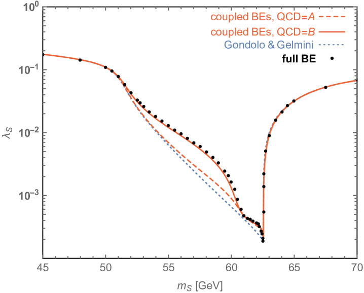
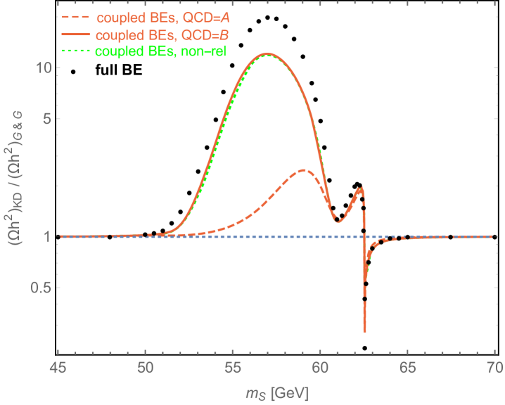
Moreover, the cBEs (6,2.1) provides a qualitatively and often quantitatively very good description for the final DM abundance, capturing most, if not all, of the effect of the kinetic decoupling. Nevertheless, for high-precision results one needs to actually solve the full Boltzmann equation in phase-space. This is because, as the full numerical solution reveals, the shape of $f_{\chi}(p)$ can be quite different from the Maxwell-Boltzmann form, which can introduce departure from the assumptions used in the cBEs. This can have a seizable impact on the result for the relic density (as for $m_{S}\sim 57$ GeV) or a very modest one (as for $m_{S}\sim m_{h}/2$) depending on whether or not the shape during chemical freeze-out is affected for momenta that can combine to $\sqrt{s}\sim m_{h}$.

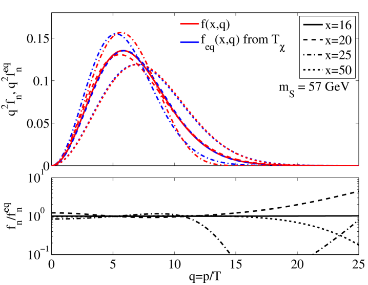
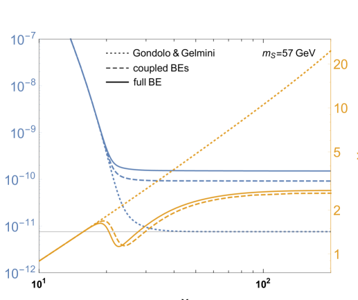
For illustration, in Fig. 2 we take an example case of $m_{S}=57$ GeV and show the full phase-space distribution for a few representative values of $x$ as well as the corresponding evolution of $Y$ and $y$. This parameter point exhibits a relatively large difference between full solution and cBEs, as visible in Fig. 1. Fig. 2 shows that this difference arises because of the dip in the ratio of DM phase-space distributions that starts to develop around the freeze-out time, for $x\gtrsim 20$. This dip in turn originates due to the resonance enhancing the annihilation in this momentum range for these $x$ values. As seen on the right panel of Fig. 2, this results in the DM particles falling out of chemical equilibrium earlier, and therefore enhance the value of the thermal relic density. It is important to stress that the bulk of this effect is well captured by the cBEs (compare the dashed vs. solid lines in the right panel of Fig. 2).

References

- [1] P. Gondolo and G. Gelmini, Nucl. Phys. B 360 (1991) 145.
- [2] T. Binder, T. Bringmann, M. Gustafsson and A. Hryczuk, Phys. Rev. D 96 (2017) 115010
- [3] V. Silveira and A. Zee, Phys. Lett. 161B (1985) 136.
- [4] T. Bringmann and S. Hofmann, JCAP 0704 (2007) 016
- [5] T. Binder, L. Covi, A. Kamada, H. Murayama, T. Takahashi and N. Yoshida, JCAP 1611 (2016) 043
- [6] P. Gondolo, J. Hisano and K. Kadota, Phys. Rev. D 86 (2012) 083523
- [7] P. Athron et al. [GAMBIT Collaboration], Eur. Phys. J. C 77 (2017) no.8, 568
- [8] J. M. Cline, K. Kainulainen, P. Scott and C. Weniger, Phys. Rev. D 88 (2013) 055025 Erratum: [Phys. Rev. D 92 (2015) no.3, 039906]
- [9] D. Boyanovsky, H. J. de Vega and D. J. Schwarz, Ann. Rev. Nucl. Part. Sci. 56 (2006) 441
- [10] M. Duch and B. Grzadkowski, JHEP 1709 (2017) 159
- [11] T. Binder, M. Gustafsson, A. Kamada, S. M. R. Sandner and M. Wiesner, arXiv:1712.01246 [astro-ph.CO].
- [12] T. Binder, T. Bringmann, M. Gustafsson and A. Hryczuk, work in progress