Data-Driven Control of Complex Networks

Giacomo Baggio Department of Information Engineering, University of Padova, Padova, Italy Danielle S. Bassett Departments of Bioengineering, Physics & Astronomy, Electrical & Systems Engineering, Neurology, and Psychiatry, University of Pennsylvania, Philadelphia, USA
Santa Fe Institute, Santa Fe, USA Fabio Pasqualetti Department of Mechanical Engineering, University of California at Riverside, Riverside, USA
To whom correspondence should be addressed: fabiopas@engr.ucr.edu

Abstract

Our ability to manipulate the behavior of complex networks depends on the design of efficient control algorithms and, critically, on the availability of an accurate and tractable model of the network dynamics. While the design of control algorithms for network systems has seen notable advances in the past few years, knowledge of the network dynamics is a ubiquitous assumption that is difficult to satisfy in practice, especially when the network topology is large and, possibly, time-varying. In this paper we overcome this limitation, and develop a data-driven framework to control a complex dynamical network optimally and without requiring any knowledge of the network dynamics. Our optimal controls are constructed using a finite set of experimental data, where the unknown complex network is stimulated with arbitrary and possibly random inputs. In addition to optimality, we show that our data-driven formulas enjoy favorable computational and numerical properties even compared to their model-based counterpart. Although our controls are provably correct for networks with linear dynamics, we also characterize their performance against noisy experimental data and in the presence of nonlinear dynamics, as they arise when mitigating cascading failures in power-grid networks and when manipulating neural activity in brain networks.

I Introduction

With the development of sensing, processing, and storing capabilities of modern sensors, massive volumes of information-rich data are now rapidly expanding in many physical and engineering domains, ranging from robotics SL-PP-AK-JI-DQ:18 , to biological VM:13 ; TJS-PSC-JAM:14 and economic sciences LE-JL:14 . Data are often dynamically generated by complex interconnected processes, and encode key information about the structure and operation of these networked phenomena. Examples include temporal recordings of functional activity in the human brain NBT:13 , phasor measurements of currents and voltages in the power distribution grid AB:10 , and streams of traffic data in urban transportation networks YL-YD-WK-ZL-FYW:14 . When first-principle models are not conceivable, costly, or difficult to obtain, this unprecedented availability of data offers a great opportunity for scientists and practitioners to better understand, predict, and, ultimately, control the behavior of real-world complex networks.

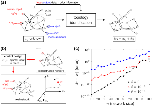
Existing works on the controllability of complex networks have focused exclusively on a model-based setting YYL-JJS-ALB:11 ; FP-SZ-FB:13q ; NB-GB-SZ:17 ; GY-GT-BB-JS-YL-AB:15 ; SG-FP-MC-QKT-BYA-AEK-JDM-JMV-MBM-STG-DSB:15 ; YYL-ALB:16 ; GL-CA:16 , although, in practice, constructing accurate models of large-scale networks is a challenging, often unfeasible, task JC-SW:08 ; SGS-MT:11 ; MTA-JAM-GL-ALB-YYL:17 . In fact, errors in the network model (i.e., missing or extra links, incorrect link weights) are unavoidable, especially if the network is identified from data (see, e.g., DA-AC-DK-CM:09 ; MSH-KJG:10 and Fig. 1(a)). This uncertainty is particularly important for network controllability, since, as exemplified in Fig. 1(b)-(c), the computation of model-based network controls tends to be unreliable and highly sensitive to model uncertainties, even for moderate size networks JS-AEM:13 ; LZW-YZC-WXW-YCL:17 . It is therefore natural to ask whether network controls can be learned directly from data, and, if so, how well these data-driven control policies perform.

Refer to caption — Figure 1: The effect of model uncertainty in the computation of optimal network controls. Panel (a) shows a schematic of a classic network identification procedure. The reconstructed network is affected by estimation errors $\delta_{ij}$ . Panel (b) illustrates the error in the final state induced by an optimal control design based on the reconstructed network. In panel (c), we consider minimum-energy controls designed from exact and incorrectly reconstructed networks, and compute the resulting error in the final state as the network size $n$ varies. We consider connected Erdös–Rényi networks with edge probability $p=\ln n/n+0.1$ , $10$ randomly selected control nodes, control horizon $T=2n$ , and a randomly chosen final state ${x}_{\textup{f}}$ . Each curve represents the average of the error in the final state over 100 random realizations. To mimic errors in the network reconstruction process, we add to each edge of the network a disturbance modeled as an i.i.d. random variable uniformly distributed in $[-\delta,\delta]$ , $\delta>0$ . To compute minimum-energy control inputs, we use the classic Gramian-based formula and standard LAPACK linear algebra routines (see Methods).

Data-driven control of dynamical systems has attracted increasing interest over the last few years, triggered by recent advances and successes in machine learning and artificial intelligence SL-CF-TD-PA:16 ; DS-et-al:17 . The classic (indirect) approach to learn controls from data is to use a sequential system identification and control design procedure. That is, one first identifies a model of the system from the available data, and then computes the desired controls using the estimated model MG:05 . However, identification algorithms are sometimes inaccurate and time-consuming, and several direct data-driven methods have been proposed to bypass the identification step (SLB-JNK:19, , Ch. III.10). These include, among others, (model-free) reinforcement learning FLL-DV-KGV:12 ; BR:18 , iterative learning control DAB-MT-AGA:06 , adaptive and self-tuning control KJA-BW:73 , and behavior-based methods IM-PR:08 ; CDP-PT:19 .

The above techniques differ in the data generation procedure, class of system dynamics considered, and control objectives. In classic reinforcement learning settings, data are generated online and updated under the guidance of a policy evaluator or reward simulator, which in many applications is represented by an offline-trained (deep) neural network DPB-JNT:96 . Iterative learning control is used to refine and optimize repetitive control tasks: data are recorded online during the execution of a task repeated multiple times, and employed to improve tracking accuracy from trial to trial. In adaptive control, the structure of the controller is fixed and a few control parameters are optimized using data collected on the fly. A widely known example is the auto-tuning of PID controllers KJA-TH:95 . Behavior-based techniques exploit a trajectory-based (or behavioral) representation of the system, and data that typically consist of a single, noiseless, and sufficiently long input-output system trajectory CDP-PT:19 . Each of the above data-driven approaches has its own limitations and merits, which strongly depend on the intended application area. However, a common feature of all these approaches is that they are tailored to or have been employed for closed-loop control tasks, such as stabilization or tracking, and not for finite-time point-to-point control tasks.

In this paper, we address the problem of learning from data point-to-point optimal controls for complex dynamical networks. Precisely, following recent literature on the controllability of complex networks JG-YYL-RMD-ALB:14 ; IK-AS-FS:17b , we focus on control policies that optimally steer the state of (a subset of) network nodes from a given initial value to a desired final one within a finite time horizon. To derive analytic, interpretable results that capture the role of the network structure, we consider networks governed by linear dynamics, quadratic cost functions, and data consisting of a set of control experiments recorded offline. Importantly, experimental data are not required to be optimal, and can even be generated through random control experiments. In this setting, we establish closed-form expressions of optimal data-driven control policies to reach a desired target state and, in the case of noiseless data, characterize the minimum number of experiments needed to exactly reconstruct optimal control inputs. Further, we introduce suboptimal yet computationally simple data-driven expressions, and discuss the numerical and computational advantages of using our data-driven approach when compared to the classic model-based one. Finally, we illustrate with different numerical studies how our framework can be applied to restore the correct operation of power-grid networks after a fault, and to characterize the controllability properties of functional brain networks.

While the focus of this paper is on designing optimal control inputs, the expressions derived in this work also provide an alternative, computationally reliable, and efficient way of analyzing the controllability properties of large network systems. This constitutes a significant contribution to the extensive literature on the model-based analysis of network controllability, where the limitations imposed by commonly used Gramian-based techniques limit the investigation to small and well-structured network topologies JS-AEM:13 ; LZW-YZC-WXW-YCL:17 .

II Results

II.1 Network dynamics and optimal point-to-point control

We consider networks governed by linear time-invariant dynamics

	$\displaystyle x(t+1)$	$\displaystyle=Ax(t)+Bu(t),$		(1)
	$\displaystyle y(t)$	$\displaystyle=Cx(t),$		(1)

where $x(t)\in\mathbb{R}^{n}$ , $u(t)\in\mathbb{R}^{m}$ , and $y(t)\in\mathbb{R}^{p}$ denote, respectively, the state, input, and output of the network at time $t$ . The matrix $A\in\mathbb{R}^{n\times n}$ describes the (directed and weighted) adjacency matrix of the network, and the matrices $B\in\mathbb{R}^{n\times m}$ and $C\in\mathbb{R}^{p\times n}$ , respectively, are typically chosen to single out prescribed sets of input and output nodes of the network.

In this work, we are interested in designing open-loop control policies that steer the network output $y(t)$ from an initial value $y(0)=y_{0}$ to a desired one $y(T)={y}_{\textup{f}}$ in $T$ steps. If ${y}_{\textup{f}}$ is output controllable TK:80 ; JG-YYL-RMD-ALB:14 (a standing assumption in this paper), then the latter problem admits a solution and, in fact, there are many ways to accomplish such a control task. Here, we assume that the network is initially relaxed ( $x(0)=0$ ), and we seek the control input $\smash{u^{\star}_{0:T-1}=[u^{\star}(T-1)^{\mathsf{T}}\cdots\,u^{\star}(0)^{\mathsf{T}}]^{\mathsf{T}}}$ that drives the output of the network to ${y}_{\textup{f}}$ in $T$ steps and, at the same time, minimizes a prescribed quadratic combination of the control effort and locality of the controlled trajectories.

Mathematically, we study and solve the following constrained minimization problem:

	$\displaystyle u^{\star}_{0:T-1}=\arg\min_{u_{0:T-1}}$	$\displaystyle y_{1:T-1}^{\mathsf{T}}\,Q\,y_{1:T-1}+u_{0:T-1}^{\mathsf{T}}\,R\,u_{0:T-1}$		(2)
		$\displaystyle\quad\text{s.t. }\ \eqref{eq:sys}\ \text{ and }\ y_{T}={y}_{\textup{f}},$		(2)

where $Q\succeq 0$ and $R\succ 0$ are tunable matrices¹¹1We let $A\succ(\succeq)\,0$ denote a positive definite (semi-definite) matrix, and $A^{\mathsf{T}}$ the transpose of $A$ . that penalize output deviation and input usage, respectively, and subscript $\cdot_{t_{1}:t_{2}}$ denotes the vector containing the samples of a trajectory in the time window $[t_{1},t_{2}]$ , $t_{1}\leq t_{2}$ (if $t_{1}=t_{2}$ , we simply write $\cdot_{t_{1}}$ ). If $Q=0$ and $R=I$ , then $u^{\star}_{0:T-1}$ coincides with the minimum-energy control to reach ${y}_{\textup{f}}$ in $T$ steps TK:80 .

Equation (2) admits a closed-form solution whose computation requires the exact knowledge of the network matrix $A$ and suffers from numerical instabilities (Methods). In the following section, we address this limitation by deriving model-free and reliable expressions of $u^{\star}_{0:T-1}$ that solely rely on experimental data collected during the network operation.

II.2 Learning optimal controls from non-optimal data

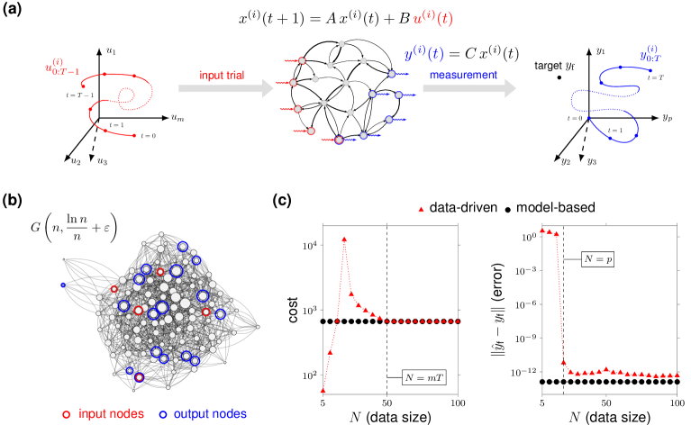
We assume that the network matrix $A$ is unknown and that $N$ control experiments have been performed with the dynamical network in (1). The $i$ -th experiment consists of generating and applying the input sequence $\smash{u_{0:T-1}^{(i)}}$ , and measuring the resulting output trajectory $\smash{y_{0:T}^{(i)}}$ (Fig. 2(a)). Here, as in, e.g., SD-HM-NM-BR-ST:18 , we consider episodic experiments where the network state is reset to zero before running a new trial, and refer to the Supplement for an extension to the non-episodic setting and to the case of episodic experiments with non-zero initial state resets. We let $U_{0:T-1}$ , $Y_{1:T-1}$ , and $Y_{T}$ denote the matrices containing, respectively, the experimental inputs, the output measurements in the time interval $[1,T-1]$ , and the output measurements at time $T$ . Namely,

$\displaystyle U_{0:T-1}$	$\displaystyle=\left[u_{0:T-1}^{(1)}\ \ \cdots\ \ u_{0:T-1}^{(N)}\right],$	(3)
$\displaystyle Y_{1:T-1}$	$\displaystyle=\left[y_{1:T-1}^{(1)}\ \ \cdots\ \ y_{1:T-1}^{(N)}\right],$
$\displaystyle Y_{T}$	$\displaystyle=\Big{[}y^{(1)}_{T}\ \ \cdots\ \ y^{(N)}_{T}\Big{]}.$

An important aspect of our analysis is that we do not require the input experiments to be optimal, in the sense of (2), nor do we investigate the problem of experiment design, i.e., generating data that are “informative” for our problem. In our setting, data are given, and these are generated from arbitrary, possibly random, or carefully chosen experiments.

By relying on the data matrices in (3), we derive the following data-driven solution to the minimization problem in (2) (see the Supplement):

\hat{u}_{0:T-1}=U_{0:T-1}(I-K_{Y_{T}}(LK_{Y_{T}})^{{\dagger}}L)Y_{T}^{{\dagger}}\,{y}_{\textup{f}},

(4)

where $L$ is any matrix satisfying $L^{\mathsf{T}}L=Y_{1:T-1}^{\mathsf{T}}QY_{1:T-1}+U_{0:T-1}^{\mathsf{T}}RU_{0:T-1}$ , $K_{Y_{T}}$ denotes a matrix whose columns form a basis of the kernel of $Y_{T}$ , and the superscript symbol $\cdot^{{\dagger}}$ stands for the Moore–Penrose pseudoinverse operation AB-TNEG:03 .

II.2.1 Minimum number of data to learn optimal controls

Finite data suffices to exactly reconstruct the optimal control input via the data-driven expression in (4) (see the Supplement). In Fig. 2(c), we illustrate this fact for the class of Erdös–Rényi networks of Fig. 2(b). Specifically, the data-driven input $\hat{u}_{0:T-1}$ equals the optimal one $u^{\star}_{0:T-1}$ (for any target ${y}_{\textup{f}}$ ) if the data matrices in (3) contain $mT$ linearly independent experiments; that is, if $U_{0:T-1}$ is full row rank (Fig. 2(c), left). We stress that linear independence of the control experiments is a mild condition that is normally satisfied when the experiments are generated randomly. Further, if the number of independent trials is smaller than $mT$ but larger than or equal to $p$ , the data-driven control $\hat{u}_{0:T-1}$ still correctly steers the network output to ${y}_{\textup{f}}$ in $T$ steps (Fig. 2(c), right), but with a cost that is typically larger than the optimal one. In this case, $\hat{u}_{0:T-1}$ is a suboptimal solution to (2), which becomes optimal (for any ${y}_{\textup{f}}$ ) if the collected data contain $p$ independent trials that are optimal as well.

II.2.2 Data-driven minimum-energy control

By letting $Q=0$ and $R=I$ in (4), we recover a data-driven expression for the $T$ -step minimum-energy control to reach ${y}_{\textup{f}}$ . We remark that the family of minimum-energy controls has been extensively employed to characterize the fundamental capabilities and limitations of controlling networks, e.g., see FP-SZ-FB:13q ; GY-GT-BB-JS-YL-AB:15 ; GL-CA:16 . After some algebraic manipulations, the data-driven minimum-energy control input can be compactly rewritten as (see the Supplement)

\hat{u}_{0:T-1}=(Y_{T}U_{0:T-1}^{{\dagger}})^{{\dagger}}\,{y}_{\textup{f}}.

(5)

The latter expression relies on the final output measurements only (matrix $Y_{T}$ ) and, thus, it does not exploit the full output data (matrix $Y_{1:T-1}$ ). Equation (5) can be further approximated as

\hat{u}_{0:T-1}\approx U_{0:T-1}Y_{T}^{{\dagger}}\,{y}_{\textup{f}}.

(6)

This is a simple, suboptimal data-based control sequence that correctly steers the network to ${y}_{\textup{f}}$ in $T$ steps, as long as $p$ independent data are available. Further, and more importantly, when the input data samples are drawn randomly and independently from a distribution with zero mean and finite variance, (6) converges to the minimum-energy control in the limit of infinite data (see the Supplement).

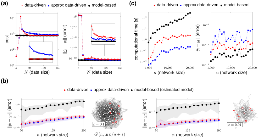
Fig. 3(a) compares the performance (in terms of control effort and error in the final state) of the two data-driven expressions (5) and (6), and the model-based control as a function of the data size $N$ . While the data-driven control in (5) becomes optimal for a finite number of data (precisely, for $N=mT$ ), the approximate expression (6) tends to the optimal control only asymptotically in the number of data (Fig. 3(a), left). In both cases, the error in the final state goes to zero after collecting $N=p$ data (Fig. 3(a), right). For the approximate control (6), we also establish upper bounds on the size of the dataset to get a prescribed deviation from the optimal cost in the case of Gaussian noise. Our non-asymptotic analysis indicates that this deviation is proportional to the worst-case control energy required to reach a unit-norm target. This, in turn, implies that networks that are “easy” to control require fewer trials to attain a prescribed approximation error (see the Supplement).

II.2.3 Numerical and computational benefits of data-driven controls

By relying on the same set of experimental data, in Fig. 3(b), we compare the numerical accuracy, as measured by the error in the final state, of the data-driven controls (5) and (6) and the minimum-energy control computed via a standard two-step approach comprising a network identification step followed by model-based control design. First, we point out that if some nodes of the network are not accessible $(C\neq I)$ and no prior information about the network structure is available, then it is impossible to exactly reconstruct the network matrix $A$ using (any number of) data PPE-VC-SW:13 . In contrast, the computation of minimum-energy inputs is always feasible via our data-driven expression, provided that enough data are collected. We thus focus on the case in which all nodes can be accessed ( $C=I$ ). We consider Erdös–Rényi networks with $n$ nodes as in Fig. 2(b) and we select $m=\lfloor n/10\rfloor$ control nodes (forming matrix $B$ ). To reconstruct the network matrices $A$ and $B$ , the subspace-based identification technique described in Methods. Data-driven strategies significantly outperform the standard sequential approach for both dense (Fig. 3(b), top) and sparse topologies (Fig. 3(b), bottom). This poor performance of the standard approach is somehow expected because, independently of the network identification procedure, the standard two-step approach requires a number of operations larger than those required by the data-driven approach, resulting in a potentially higher sensitivity to round-off errors. Also, it is interesting to note that the data-driven approach is especially effective for large, dense networks for which the standard approach leads to errors of considerable magnitude (up to approximately $10^{2}$ ).

A further advantage in using data-driven controls over model-based ones arises when dealing with massive networks featuring a small fraction of input and output nodes. Specifically, in Fig. 3(c) we plot the time needed to numerically compute the data-driven and model-based controls as a function of the size of the network. We focus on Erdös–Rényi networks as in Fig. 2(b) of dimension $n\geq 1000$ with $\lfloor n/100\rfloor$ input and output nodes and a control horizon $T=50$ . The model-based control input requires the computation of the first $T-1$ powers of $A$ (Methods). The computation of the data-driven expressions (5) and (6) involves, instead, linear-algebraic operations on two matrices ( $U_{0:T-1}$ and $Y_{T}$ ) that are typically smaller than $A$ when $n$ is very large (precisely, when $T<n/m$ and $N<n$ ). Thus, the computation of the control input via the data-driven approach is normally faster than the classic model-based computation (Fig. 3(c), left). In particular, the data-driven control (6), although suboptimal, yields the most favorable performance due to its particularly simple expression. Finally, we note that the error in the final state committed by the data-driven controls is always upper bounded by $10^{-5}$ and thus it has a negligible effect on the control accuracy (Fig. 3(c), right).

II.2.4 Data-driven controls with noisy data

The analysis so far has focused on noiseless data. A natural question is how the data-driven controls behave in the case of noisy data. If the noise is unknown but small in magnitude, then the established data-driven expressions will deviate slightly from the correct values (see the Supplement). However, if some prior information on the noise is known, this information can be exploited to return more accurate control expressions. A particularly relevant case is when data are corrupted by additive i.i.d. noise with zero mean and known variance.²²2The different types of noise are assumed to be zero-mean to simplify the exposition. With slight modifications, non zero-mean noise could also be accommodated by our approach. Namely, the available data read as

$\displaystyle U_{0:T-1}$	$\displaystyle=\bar{U}_{0:T-1}+\Delta_{U},$	(7)
$\displaystyle Y_{1:T-1}$	$\displaystyle=\bar{Y}_{1:T-1}+\Delta_{Y},$
$\displaystyle Y_{T}$	$\displaystyle=\bar{Y}_{T}+\Delta_{Y_{T}},$

where $\bar{U}_{0:T-1}$ , $\bar{Y}_{1:T-1}$ , $\bar{Y}_{T}$ denote the ground truth values and $\Delta_{U}$ , $\Delta_{Y}$ , and $\Delta_{Y_{T}}$ are random matrices with i.i.d. entries with zero mean and variance $\sigma_{U}^{2}$ , $\sigma_{Y}^{2}$ , and $\sigma_{Y_{T}}^{2}$ , respectively. Note that the noise terms $\Delta_{Y}$ and $\Delta_{Y_{T}}$ may also include the contribution of process noise acting on the network dynamics. In this setting, it can be shown that the data-driven control (4) and the data-driven minimum-energy controls (5) and (6) are typically not consistent; that is, they do not converge to the true control inputs as the data size tends to infinity (see the Supplement for a concrete example). However, by suitably modifying these expressions, it is possible to recover asymptotically correct data-driven formulas (Supplement). The key idea is to add correction terms that compensate for the noise variance arising from the pseudoinverse operations. In particular, the asymptotically correct version of the data-driven controls (5) and (6) read, respectively, as

	$\displaystyle\hat{u}^{\prime}_{0:T-1}$	$\displaystyle=$	$\displaystyle(Y_{T}U_{0:T-1}^{\mathsf{T}}(U_{0:T-1}U_{0:T-1}^{\mathsf{T}}-N\sigma_{U}^{2}I)^{{\dagger}})^{{\dagger}}{y}_{\textup{f}},$		(8)
	$\displaystyle\hat{u}^{\prime\prime}_{0:T-1}$	$\displaystyle=$	$\displaystyle U_{0:T-1}Y_{T}^{\mathsf{T}}(Y_{T}Y_{T}^{\mathsf{T}}-N\sigma^{2}_{Y_{T}}I)^{{\dagger}}\,{y}_{\textup{f}},$		(9)

where we used the fact that $X^{{\dagger}}=X^{\mathsf{T}}(XX^{\mathsf{T}})^{{\dagger}}$ for any matrix $X$ AB-TNEG:03 , and $N\sigma_{U}^{2}I$ and $N\sigma_{Y_{T}}^{2}I$ represent the noise-dependent correction terms. Note, in particular, that if the noise corrupts the output data $Y_{T}$ only, then (8) coincides with the original data-driven control (5), so that no correction is needed. Similarly, if the noise corrupts the input data $U_{T}$ only, then (9) coincides with the data-driven control (6).

II.3 Applications

To demonstrate the potential relevance and applicability of the data-driven framework presented thus far, we present two applications of our data-driven control formulas.

II.3.1 Data-driven fault recovery in power-grid networks

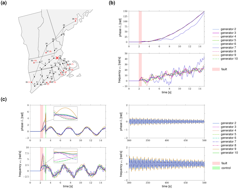
We address the problem of restoring the normal operation of a power-grid network after the occurrence of a fault which desynchronizes part of the grid. If not mitigated in a timely manner, such desynchronization instabilities may trigger cascading failures that can ultimately cause major blackouts and grid disruptions YS-IM-TH:11 ; SPC-LWK-AEM:13 ; JWSP-FD-FB:16 . In our case study, we consider a line fault in the New England power grid network comprising 39 nodes (29 load nodes and 10 generator nodes), as depicted in Fig. 4(a), and we compute an optimal point-to-point control from data to recover the correct operation of the grid. A similar problem is solved in SPC-LWK-AEM:13 using a more sophisticated control strategy which requires knowledge of the network dynamics. As in YS-IM-TH:11 ; SPC-LWK-AEM:13 , we assume that the phase $\delta_{i}$ and the (angular) frequency $\omega_{i}$ of each generator $i$ obey the swing equation dynamics with the parameters given in YS-IM-TH:11 (except for generator 1 whose phase and frequency are fixed to a constant, cf. Methods). Initially, each generator operates at a locally stable steady-state condition determined by the power flow equations. At time $t=2$ s, a three-phase fault occurs in the transmission line connecting nodes 16 and 17. After $0.5$ s the fault is cleared; however the generators have lost synchrony and deviate from their steady-state values (Fig. 4(b)). To recover the normal behavior of the grid, $0.5$ s after the clearance of the fault, we apply a short, optimal control input to the frequency of the generators to steer the state (phase and frequency) of the generators back to its steady-state value. The input is computed from data via (4) using $N=4000$ input/state experiments collected by locally perturbing the state of the generators around its normal operation point (see also Methods). We consider data sampled with period $T_{s}=2.5\times 10^{-4}$ s, and set the control horizon to $T=400$ time samples (corresponding to $0.1$ s), $R=I$ , and $Q=\varepsilon I$ with $\varepsilon=0.01$ to enforce locality of the controlled trajectories. As shown in Fig. 4(c), the data-driven input drives the state of the generators to a point close enough to the starting synchronous solution (left, inset) so as to asymptotically recover the correct operation of the grid (right). Notably, as previously discussed, the computation of the control input requires only pre-collected data, is numerically efficient, and optimal (for the linearized dynamics). More generally, this numerical study suggests that the data-driven strategy (4) could represent a simple, viable, and computationally-efficient approach to control complex non-linear networks around an operating point.

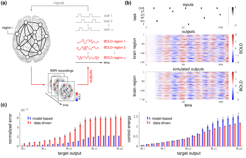
II.3.2 Controlling functional brain networks via fMRI snapshots

We investigate the problem of generating prescribed patterns of activity in functional brain networks directly from task-based functional magnetic resonance imaging (task-fMRI) time series. Specifically, we examine a dataset of task-based fMRI experiments related to motor activity extracted from the Human Connectome Project (HCP) DCVE-et-al:13 (see Fig. 5(a)). In these experiments, participants are presented with visual cues that ask them to execute specific motor tasks; namely, tap their left or right fingers, squeeze their left or right toes, and move their tongue. We consider a set of $m=6$ input channels associated with different task-related stimuli; that is, the motor tasks’ stimuli and the visual cue preceding them. As in CO-DSB-VMP:18 , we encode the input signals as binary time series taking the value of 1 when the corresponding task-related stimulus occurs and 0 otherwise. The output signals consist of minimally pre-processed blood-oxygen-level-dependent (BOLD) time series associated with the fMRI measurements at different regions of the brain (see also Methods). In our numerical study, we parcellated the brain into $p=148$ brain regions (74 regions per hemisphere) according to the Destrieux 2009 atlas CD-BF-AD-EH:10 . Further, as a baseline for comparison, we approximate the dynamics of the functional network with a low-dimensional ( $n=20$ ) linear model computed via the approach described in CO-DSB-VMP:18 , which has been shown to accurately capture the underlying network dynamics.

In Fig. 5(b), we plot the inputs (top) and outputs (center) of one subject for the first sequence of five motor tasks. The bottom plot of the same figure shows the outputs obtained by approximating the network dynamics with the above-mentioned linear model. In Fig. 5(c), we compare the performance of the minimum-energy data-driven control in (5) with the model-based one, assuming that the network obeys the dynamics of the approximate linear model. We choose a control horizon $T=100$ , form the data matrices in (3) by sliding a window of fixed size $T$ over the available fMRI data, and consider a set of 20 orthogonal targets $\{y_{\text{f},i}\}_{i=1}^{20}$ corresponding to eigenvectors of the estimated $T$ -step controllability Gramian (see Methods for further details). The top plot of Fig. 5(c) reports the error (normalized by the output dimension) in the final state of the two strategies, while the bottom plot shows the corresponding control energy (that is, the norm of the control input). In the plots, the targets are ordered from the most ( $y_{\text{f},1}$ ) to the least ( $y_{\text{f},20}$ ) controllable. The data-driven and the model-based inputs exhibit an almost identical behavior with reference to the most controllable targets. As we shift towards the least controllable targets, the data-driven strategy yields larger errors but, at the same time, requires less energy to be implemented, thus being potentially more feasible in practice. Importantly, since the underlying brain dynamics are not known, errors in the final state are computed using the identified linear dynamical model. It is thus expected that data-driven inputs yield larger errors in the final state than model-based inputs, although these errors may not correspond to control inaccuracies when applying the data-driven inputs to the actual brain dynamics. Ultimately, our numerical study suggests that the data-driven framework could represent a viable alternative to the classic model-based approach (e.g., see SG-FP-MC-QKT-BYA-AEK-JDM-JMV-MBM-STG-DSB:15 ; SD-SG:20 ; TM-GB-DSB-FP:19b ) to infer controllability properties of brain networks, and (by suitably modulating the reconstructed inputs) enforce desired functional configurations in a non-invasive manner and without requiring real-time measurements.

III Discussion

In this paper we present a framework to control complex dynamical networks from data generated by non-optimal (and possibly random) experiments. We show that optimal point-to-point controls to reach a desired target state, including the widely used minimum-energy control input, can be determined exactly from data. We provide closed-form and approximate data-based expressions of these control inputs and characterize the minimum number of samples needed to compute them. Further, we show by means of numerical simulations that data-driven inputs are more accurate and computationally more efficient than model-based ones, and can be used to analyze and manipulate the controllability properties of real networks.

More generally, our framework and results suggest that many network control problems may be solved by simply relying on experimental data, thus promoting a new, exciting, and practical line of research in the field of complex networks. Because of the abundance of data in modern applications and the computationally appealing properties of data-driven controls, we expect that this new line of research will benefit a broad range of research communities, spanning from engineering to biology, which employ control-theoretic methods and tools to comprehend and manipulate complex networked phenomena.

Some limitations of this study should also be acknowledged and discussed. First, in our work we consider networks governed by linear dynamics. On the one hand, this is a restrictive assumption since many real-world networks are inherently nonlinear. On the other hand, linear models are used successfully to approximate the behavior of nonlinear dynamical networks around desired operating points, and capture more explicitly the impact of the network topology. Second, in many cases a closed-loop control strategy is preferable than a point-to-point one, especially if the control objective is to stabilize an equilibrium when external disturbances corrupt the dynamics. However, we stress that point-to-point controls, in addition to being able to steer the network to arbitrary configurations, are extensively used to characterize the fundamental control properties and limitations in networks of dynamical nodes. For instance, the expressions we provide for point-to-point control can also lead to novel methods to study the energetic limitations of controlling complex networks FP-SZ-FB:13q , select sensors and actuators for optimized estimation and control THS-FLC-JL:16 , and design optimized network structures SZ-FP:16a . Finally, although we provide data-driven expressions that compensate for the effect of noise in the limit of infinite data, we do not provide non-asymptotic guarantees on the reconstruction error. Overcoming these limitations represents a compelling direction of future work, which can strengthen the relevance and applicability of our data-driven control framework, and ultimately lead to viable control methods for complex networks.

IV Methods

IV.1 Model-based expressions of optimal controls

The model-based solution to (2) can be written in batch form as

u^{\star}_{0:T-1}=(I-K_{\mathcal{C}_{T}}(MK_{\mathcal{C}_{T}})^{\dagger}M)\mathcal{C}_{T}^{\dagger}{y}_{\textup{f}},

(10)

where $\mathcal{C}_{T}=[CB\ CAB\ \cdots\ CA^{T-1}B]$ is the $T$ -step output controllability matrix of the dynamical network in (1), $K_{Y_{T}}$ denotes a basis of the kernel of $\mathcal{C}_{T}$ , and $M$ is any matrix satisfying $M^{\mathsf{T}}M=\mathcal{H}_{T}^{\mathsf{T}}Q\mathcal{H}_{T}+R$ , with

\displaystyle\mathcal{H}_{T}=\begin{bmatrix}0&\cdots&\cdots&0&CB\\ \vdots&\cdots&0&CB&CAB\\ \vdots&\iddots&\iddots&\iddots&\vdots\\ 0&CB&CAB&\cdots&CA^{T-2}B\\ \end{bmatrix},

and $0$ entries denoting $p\times m$ zero matrices. If $Q=0$ and $R=I$ (minimum-energy control input), (10) simplifies to $u^{\star}_{0:T-1}=\mathcal{C}_{T}^{\dagger}{y}_{\textup{f}}$ . Alternatively, if the network is target controllable, the minimum-energy input can be compactly written as

u^{\star}(t)=B^{\mathsf{T}}A^{T-t-1}C^{\mathsf{T}}\mathcal{W}_{T}^{-1}{y}_{\textup{f}},\quad t=0,1,2,\dots,T-1.

(11)

where $\mathcal{W}_{T}$ denotes the $T$ -step output controllability Gramian of the dynamical network in (1)

\mathcal{W}_{T}=\mathcal{C}_{T}\mathcal{C}_{T}^{\mathsf{T}}=\sum_{t=0}^{T-1}CA^{t}BB^{\mathsf{T}}(A^{\mathsf{T}})^{t}C^{\mathsf{T}},

(12)

which is invertible if and only if the network is target controllable. Equation (11) is the classic (Gramian-based) expression of the minimum-energy control input TK:80 . It is well-known that this expression is numerically unstable, even for moderate size systems, e.g., see JS-AEM:13 .

IV.2 Subspace-based system identification

Given the data matrices $U_{0:T-1}$ and $Y_{T}$ as defined in (3) and assuming that $C=I$ , a simple deterministic subspace-based procedure (TK:05, , Ch. 6) to estimate the matrices $A$ and $B$ from the available data consists of the following two steps:

1.

Compute an estimate of the $T$ -step controllability matrix of the network as the solution of the minimization problem

$\hat{\mathcal{C}}_{T}=\arg\min_{\mathcal{C}_{T}}\left\|Y_{T}-{\mathcal{C}_{T}}U_{0:T-1}\right\|^{2}_{\text{F}},$ (13)

where $\|\cdot\|_{\text{F}}$ denotes the Frobenius norm of a matrix. The solution to (13) has the form $\hat{\mathcal{C}}_{T}=Y_{T}U_{0:T-1}^{\dagger}$ .

In view of the definition of the controllability matrix, obtain an estimate of the matrix $B$ by extracting the first $m$ columns of $\hat{\mathcal{C}}_{T}$ . Namely, $\hat{B}=[\hat{\mathcal{C}}_{T,}]_{:,1:m}$ , where $[X]_{:,i:j}$ indicates the sub-matrix of $X$ obtained from keeping the entries from the $i$ -th to $j$ -th columns and all of its rows. An estimate of the matrix $A$ can be obtained as the solution to the least-squares problem

\hat{A}=\arg\min_{A}\left\|[\hat{\mathcal{C}}_{T}]_{:,m+1:mT}-A\,[\hat{\mathcal{C}}_{T}]_{:,1:(T-1)m}\right\|^{2}_{\text{F}},

which yields the matrix $\hat{A}=[\hat{\mathcal{C}}_{T}]_{:,m+1:mT}[\hat{\mathcal{C}}_{T}]_{:,1:(T-1)m}^{\dagger}$ .

If the data are noiseless, the system is controllable in $T-1$ steps, and $U_{0:T-1}$ has full row rank, then this procedure provably returns correct estimates of $A$ and $B$ TK:05 .

IV.3 Power-grid network dynamics, parameters, and data generation

The short-term electromechanical behavior of generators $\{2,\dots,10\}$ of the New England power-grid network are modeled by the swing equations PK:94 :

	$\displaystyle\dot{\delta}_{i}$	$\displaystyle=\omega_{i},$		(14)
	$\displaystyle\frac{H_{i}}{\pi f_{b}}\dot{\omega}_{i}$	$\displaystyle=-D_{i}\omega_{i}+P_{\text{m}i}-G_{ii}E_{i}^{2}+\sum_{j=1,j\neq i}^{10}E_{i}E_{j}\left(G_{ij}\cos(\delta_{i}-\delta_{j})+B_{ij}\sin(\delta_{i}-\delta_{j})\right).$		(14)

where $\delta_{i}$ is the angular position or phase of the rotor in generator $i$ with respect to generator $1$ , and where $\omega_{i}$ is the deviation of the rotor speed or frequency in generator $i$ relative to the nominal angular frequency $2\pi f_{b}$ . The generator $1$ is assumed to be connected to an infinite bus, and has constant phase and frequency. The parameters $H_{i}$ and $D_{i}$ are the inertia constant and damping coefficient, respectively, of generator $i$ . The parameter $G_{ii}$ is the internal conductance of generator $i$ , and $G_{ij}+\mathrm{i}B_{ij}$ (where $\mathrm{i}$ is the imaginary unit) is the transfer impedance between generators $i$ and $j$ . The parameter $P_{\text{m}i}$ denotes the mechanical input power of generator $i$ and $E_{i}$ denotes the internal voltage of generator $i$ . The values of parameters $f_{b}$ , $H_{i}$ , $D_{i}$ , $G_{ij}$ , $B_{ij}$ , and $P_{\text{m}i}$ in the non-faulty and faulty configuration are taken from YS-IM-TH:11 , while the voltages $E_{i}$ and initial conditions ( $\delta_{i}(0)$ , $\omega_{i}(0)=0$ ) are fixed using a power flow computation. In our numerical study, we discretize the dynamics (14) using a forward Euler method with sampling time $T_{s}=2.5\times 10^{-4}$ s. Data are generated by applying a Gaussian i.i.d. perturbation with zero mean and variance $0.01$ to each frequency $\omega_{i}$ . The initial condition of each experiment is computed by adding a Gaussian i.i.d. perturbation with zero mean and variance $0.01$ to the steady-state values of $\delta_{i}$ and $\omega_{i}$ of the swing dynamics (14).

IV.4 Task-fMRI dataset, pre-processing pipeline, and identification setup

The motor task fMRI data used in our numerical study are extracted from the HCP S1200 release DCVE-et-al:13 ; HCP . The details for data acquisition and experiment design can be found in HCP . The BOLD measurements have been pre-processed according to the minimal pipeline described in MFG-et-al:13 , and, as in CO-DSB-VMP:18 , filtered with a band-pass filter to attenuate the frequencies outside the 0.06–0.12 Hz band. Further, as common practice, the effect of the physiological signals (cardiac, respiratory, and head motion signals) is removed from the BOLD measurements by means of the regression procedure in CO-DSB-VMP:18 . The data matrices in (3) are generated via a sliding window of fixed length $T=100$ with initial time in the interval $[-90,10]$ . We assume that the inputs and states are zero for times less than or equal to 10, i.e., the instant at which the first task condition is issued. We approximate the input-output dynamics with a linear model with state dimension $n=20$ computed using input-output data in the interval $[0,150]$ and the identification procedure detailed in CO-DSB-VMP:18 . When the estimated network matrix $A$ has unstable eigenvalues, we stabilize $A$ by diving it by $\rho(A)+0.01$ , where $\rho(A)$ denotes the spectral radius of $A$ . Other identification parameters are as in CO-DSB-VMP:18 .

IV.5 Computational details

All numerical simulations have been performed via standard linear-algebra LAPACK routines available as built-in functions in Matlab^® R2019b, running on a 2.6 GHz Intel Core i5 processor with 8 GB of RAM. In particular, for the computation of pseudoinverses we use the singular value decomposition method (command pinv in Matlab^®) with a threshold of $10^{-8}$ .

IV.6 Materials and data availability

Data were provided (in part) by the Human Connectome Project, WU-Minn Consortium (Principal Investigators: David Van Essen and Kamil Ugurbil; 1U54MH091657) funded by the 16 NIH Institutes and Centers that support the NIH Blueprint for Neuroscience Research; and by the McDonnell Center for Systems Neuroscience at Washington University. The code and data used in this study are freely available in the public GitHub repository: https://github.com/baggiogi/data_driven_control.

Acknowledgements

This work was supported in part by awards AFOSR-FA9550-19-1-0235 and ARO-71603NSYIP, and by MIUR (Italian Minister for Education) under the initiative “Departments of Excellence” (Law 232/2016).

Author contributions

G.B, D.S.B, and F.P. contributed to the conceptual and theoretical aspects of the study, wrote the manuscript and the Supplement. G.B. carried out the numerical studies and prepared the figures.

Competing interests

The authors declare no competing interests.

References

(1) Levine, S., Pastor, P., Krizhevsky, A., Ibarz, J. & Quillen, D. Learning hand-eye coordination for robotic grasping with deep learning and large-scale data collection. The International Journal of Robotics Research 37, 421–436 (2018).
(2) Marx, V. Biology: The big challenges of big data. Nature 498, 255–260 (2013).
(3) Sejnowski, T. J., Churchland, P. S. & Movshon, J. A. Putting big data to good use in neuroscience. Nature neuroscience 17, 1440 (2014).
(4) Einav, L. & Levin, J. Economics in the age of big data. Science 346, 1243089 (2014).
(5) Turk-Browne, N. B. Functional interactions as big data in the human brain. Science 342, 580–584 (2013).
(6) Bose, A. Smart transmission grid applications and their supporting infrastructure. IEEE Transactions on Smart Grid 1, 11–19 (2010).
(7) Lv, Y., Duan, Y., Kang, W., Li, Z. & Wang, F.-Y. Traffic flow prediction with big data: a deep learning approach. IEEE Transactions on Intelligent Transportation Systems 16, 865–873 (2014).
(8) Liu, Y. Y., Slotine, J. J. & Barabási, A. L. Controllability of complex networks. Nature 473, 167–173 (2011).
(9) Pasqualetti, F., Zampieri, S. & Bullo, F. Controllability metrics, limitations and algorithms for complex networks. IEEE Transactions on Control of Network Systems 1, 40–52 (2014).
(10) Bof, N., Baggio, G. & Zampieri, S. On the role of network centrality in the controllability of complex networks. IEEE Transactions on Control of Network Systems 4, 643–653 (2017).
(11) Yan, G. et al. Spectrum of controlling and observing complex networks. Nature Physics 11, 779–786 (2015).
(12) Gu, S. et al. Controllability of structural brain networks. Nature Communications 6 (2015).
(13) Liu, Y.-Y. & Barabási, A.-L. Control principles of complex systems. Reviews in Modern Physics 88, 035006 (2016).
(14) Lindmark, G. & Altafini, C. Minimum energy control for complex networks. Scientific Reports 8, 3188–3202 (2018).
(15) Gonçalves, J. & Warnick, S. Necessary and sufficient conditions for dynamical structure reconstruction of lti networks. IEEE Transactions on Automatic Control 53, 1670–1674 (2008).
(16) Shandilya, S. G. & Timme, M. Inferring network topology from complex dynamics. New Journal of Physics 13, 013004 (2011).
(17) Angulo, M. T., Moreno, J. A., Lippner, G., Barabási, A.-L. & Liu, Y.-Y. Fundamental limitations of network reconstruction from temporal data. Journal of the Royal Society Interface 14, 20160966 (2017).
(18) Achlioptas, D., Clauset, A., Kempe, D. & Moore, C. On the bias of traceroute sampling: or, power-law degree distributions in regular graphs. Journal of the ACM (JACM) 56, 1–28 (2009).
(19) Handcock, M. S. & Gile, K. J. Modeling social networks from sampled data. The Annals of Applied Statistics 4, 5 (2010).
(20) Sun, J. & Motter, A. E. Controllability transition and nonlocality in network control. Physical Review Letters 110, 208701 (2013).
(21) Wang, L.-Z., Chen, Y.-Z., Wang, W.-X. & Lai, Y.-C. Physical controllability of complex networks. Scientific reports 7, 40198 (2017).
(22) Levine, S., Finn, C., Darrell, T. & Abbeel, P. End-to-end training of deep visuomotor policies. The Journal of Machine Learning Research 17, 1334–1373 (2016).
(23) Silver, D. et al. Mastering the game of Go without human knowledge. Nature 550, 354 (2017).
(24) Gevers, M. Identification for control: From the early achievements to the revival of experiment design. European Journal of Control 11, 1–18 (2005).
(25) Brunton, S. L. & Kutz, J. N. Data-driven science and engineering: Machine learning, dynamical systems, and control (Cambridge University Press, 2019).
(26) Lewis, F. L., Vrabie, D. & Vamvoudakis, K. G. Reinforcement learning and feedback control: Using natural decision methods to design optimal adaptive controllers. IEEE Control Systems Magazine 32, 76–105 (2012).
(27) Recht, B. A tour of reinforcement learning: The view from continuous control. Annual Review of Control, Robotics, and Autonomous Systems (2018).
(28) Bristow, D. A., Tharayil, M. & Alleyne, A. G. A survey of iterative learning control. IEEE control systems magazine 26, 96–114 (2006).
(29) Åström, K. J. & Wittenmark, B. On self tuning regulators. Automatica 9, 185–199 (1973).
(30) Markovsky, I. & Rapisarda, P. Data-driven simulation and control. International Journal of Control 81, 1946–1959 (2008).
(31) Persis, C. D. & Tesi, P. Formulas for data-driven control: Stabilization, optimality and robustness. IEEE Transactions on Automatic Control 65, 909–924 (2020).
(32) Bertsekas, D. P. & Tsitsiklis, J. N. Neuro-dynamic programming, vol. 5 (Athena Scientific Belmont, MA, 1996).
(33) Åström, K. J. & Hägglund, T. PID controllers: theory, design, and tuning, vol. 2 (Instrument society of America Research Triangle Park, NC, 1995).
(34) Gao, J., Liu, Y.-Y., D’Souza, R. M. & Barabási, A. L. Target control of complex networks. Nature communications 5, 5415 (2014).
(35) Klickstein, I., Shirin, A. & Sorrentino, F. Energy scaling of targeted optimal control of complex networks. Nature communications 8, 15145 (2017).
(36) Kailath, T. Linear Systems (Prentice-Hall, 1980).
(37) Dean, S., Mania, H., Matni, N., Recht, B. & Tu, S. On the sample complexity of the linear quadratic regulator. Foundations of Computational Mathematics 1–47 (2019).
(38) Ben-Israel, A. & Greville, T. N. E. Generalized inverses: theory and applications, vol. 15 of CMS Books in Mathematics (Springer-Verlag New York, 2003), 2nd edn.
(39) Paré, P. E., Chetty, V. & Warnick, S. On the necessity of full-state measurement for state-space network reconstruction. In 2013 IEEE Global Conference on Signal and Information Processing, 803–806 (IEEE, 2013).
(40) Susuki, Y., Mezić, I. & Hikihara, T. Coherent swing instability of power grids. Journal of nonlinear science 21, 403–439 (2011).
(41) Cornelius, S. P., Kath, W. L. & Motter, A. E. Realistic control of network dynamics. Nature Communications 4 (2013).
(42) Simpson-Porco, J. W., Dörfler, F. & Bullo, F. Voltage collapse in complex power grids. Nature Communications 7, 1–8 (2016).
(43) Van Essen, D. C. et al. The WU-Minn human connectome project: an overview. Neuroimage 80, 62–79 (2013).
(44) Becker, C. O., Bassett, D. S. & Preciado, V. M. Large-scale dynamic modeling of task-fMRI signals via subspace system identification. Journal of neural engineering 15, 066016 (2018).
(45) Destrieux, C., Fischl, B., Dale, A. & Halgren, E. Automatic parcellation of human cortical gyri and sulci using standard anatomical nomenclature. Neuroimage 53, 1–15 (2010).
(46) Deng, S. & Gu, S. Controllability analysis of functional brain networks. arXiv preprint arXiv:2003.08278 (2020).
(47) Menara, T., Baggio, G., Bassett, D. S. & Pasqualetti, F. A framework to control functional connectivity in the human brain. In IEEE Conf. on Decision and Control, 4697–4704 (Nice, France, 2019).
(48) Summers, T. H., Cortesi, F. L. & Lygeros, J. On submodularity and controllability in complex dynamical networks. IEEE Transactions on Control of Network Systems 3, 91–101 (2016).
(49) Zhao, S. & Pasqualetti, F. Networks with diagonal controllability gramians: Analysis, graphical conditions, and design algorithms. Automatica 102, 10–18 (2019).
(50) Katayama, T. Subspace methods for system identification. Communications and Control Engineering (Springer-Verlag London, 2005).
(51) Kundur, P. Power System Stability and Control (McGraw-Hill, 1994).
(52) WU-Minn, HCP 1200 subjects data release reference manual. https://www.humanconnectome.org (2017). Accessed: 2020-03-15.
(53) Glasser, M. F. et al. The minimal preprocessing pipelines for the human connectome project. Neuroimage 80, 105–124 (2013).