Data-driven time-scale separation of ODE right-hand sides using dynamic mode decomposition and time delay embedding

Cody J. Balos
Lawrence Livermore National Laboratory

Abstract

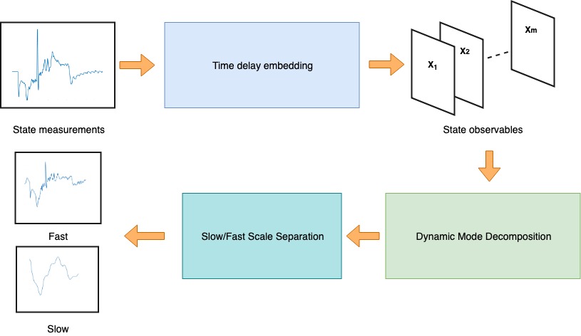
Multi-physics simulation often involve multiple different scales. The ARKODE ODE solver package in the SUNDIALS library addresses multi-scale problems with a multi-rate time-integrator that can work with a right-hand side that has fast scale and slow scale components. In this report, we use dynamic mode decomposition and time delay embedding to extract the fast and and slow components of the right-hand sides of a simple ODE from data. We then use the extracted components to solve the ODE with ARKODE. Finally, to move towards a real-world use case, we attempt to extract fast and slow scale dynamics from synthetic seismic modeling data.

$\clubsuit$

1 Introduction and Overview

As computing power increases, multi-physics simulations which involve the coupling of different physical phenomena are becoming more common and more ambitious. The different physics in these simulations often occur at different scales. As a result, there are inefficiencies when solving the ODE systems that arise because the time-step of the integrator is restricted by the fast scale. The ARKODE [6] ODE solver package in the SUNDIALS library [1] addresses these problems with a multirate time-integrator that is defined by a right-hand side composed of a fast-scale and slow-scale components as shown in Equation (1). Naturally, this leads to the question of how to split the right-hand side appropriately. In this report, we will take a data-driven approach based on the dynamic mode decomposition (DMD), a powerful tool for approximating dynamics from data [4, 7].

\dot{y}=\underbrace{f_{s}(t,y)}_{\text{slow scale}}+\underbrace{f_{f}(t,y)}_{\text{fast scale}},\quad y(t_{0})=y_{0}

(1)

In [2], Grosek et al., introduced a method for extracting the low-rank and sparse components of a DMD approximation in the context of background and foreground separation in videos, however, we will apply the concept to other dynamical systems where there exists a slow-scale (background) that is much slower than a fast-scale (foreground). In order to successfully reconstruct the dynamics from systems with only one partial state information, we will use time delay embeddings to augment the state. This method was presented by Kamb et al. as a Koopman observable in [3].

After extracting the the fast and slow components of an simple ODE right-hand side, we will solve a multi-rate ODE by feeding the approximated components into ARKODE. Finally, we will attempt to extract fast and slow-scale dynamics from synthetic tsunami modeling data produced with a code developed by Vogl and Leveque based on the Clawpack solver package [8]. The idea is that with some additional work, the extracted components could be used as the fast and slow right hand sides in ARKODE to solve ODE system(s) that stem from the wave propagation equations discussed.

The rest of this report is organized as follows. Section 2 discusses the theory behind the methods used to form our separation algorithm. Section 3 explains the algorithm and its implementation in MATLAB. Section 4 discussed the computational results for the toy problem and the synthetic tsunami data. Finally, we provide our conclusions in Section 5.

2 Theoretical Background

In this section we will discuss the theory behind the different methods used in our separation algorithm. Consider a dynamical system

\frac{d\mathbf{x}}{dt}=\mathbf{f}(\mathbf{x},t;\mu),

(2)

where $\mathbf{x}(t)\in\mathbb{R}^{n}$ is a vector representing the state of our dynamical system at time $t$ , $\mu$ contains the parameters of the system, and $\mathbf{f}(\cdot)$ represents the dynamics. By sampling (2) with a uniform sampling rate we get the discrete-time flow-map

\mathbf{x}_{k+1}=\mathbf{F}(\mathbf{x}_{k}).

(3)

2.1 Koopman Theory

The Koopman operator $\mathcal{K}_{t}$ provides an operator perspective on dynamical systems. The insight behind the operator is that the finite-dimensional, nonlinear dynamics of (2) can be transformed to an infinite-dimensional, linear dynamical system by considering a new space of scalar observable functions $g:\mathbb{R}^{N}\rightarrow\mathbb{C}$ on the state instead of the state directly [3]. The Kooopman operator acts on the observable:

\mathcal{K}_{t}g(\mathbf{x}_{0})=g(\mathbf{F}_{t}(\mathbf{x}_{0}))=g(x(t))

where $\mathcal{K}_{t}$ maps the measurement function $g$ to the next set of value it will take after time $t$ .

2.2 Dynamic Mode Decomposition

By sampling (2) with a uniform sampling rate, the DMD approximates the low-dimensional modes of the linear, time-independent Koopman operator in order to estimate the dynamics of the system. Consider $n$ data points with a total of $m$ samplings in time, then we can form the two matrices:

\mathbf{X_{1}}=\begin{bmatrix}\mid&\mid&\mid\\ \mathbf{x_{1}}&\mathbf{x_{2}}&\cdots&\mathbf{x}_{m-1}\\ \mid&\mid&\mid\end{bmatrix}

(4)

\mathbf{X_{2}}=\begin{bmatrix}\mid&\mid&\mid\\ \mathbf{x_{2}}&\mathbf{x_{3}}&\cdots&\mathbf{x}_{m}\\ \mid&\mid&\mid\end{bmatrix}.

(5)

The Koopman operator $\mathbf{A}$ provides a mapping that takes the system, modeled by the data, from time $j$ to $j+1$ , i.e. $x_{j+1}=\mathbf{A}x_{j}$ . We can use the singular value decomposition (SVD) of the matrix $\mathbf{X}_{1}$ to reduce the rank $\ell$ as well as to obtain the benefits of unitary matrices. Accordingly, $\mathbf{X_{1}}=\mathbf{U}\mathbf{\Sigma}\mathbf{V}^{*}$ , where $\mathbf{U}\in\mathbb{C}^{n\times\ell}$ is unitary, $\mathbf{\Sigma}\in\mathbb{C}^{\ell\times\ell}$ is diagonal, and $\mathbf{U}\in\mathbb{C}^{(m-1)\times\ell}$ is unitary. Thus, the approximate eigendecomposition of the Koopman operator is:

\tilde{\mathbf{A}}=\mathbf{U}^{*}\mathbf{X_{2}}\mathbf{V}\mathbf{\Sigma},

the eigenvalues are given by $\tilde{\mathbf{A}}\omega_{j}=\lambda_{j}\omega_{j}$ , and the DMD mode (eigenvector of the Koopman operator) corresponding to eigenvalue $\lambda_{j}$ is ${\varphi}_{j}=\mathbf{U}\omega_{j}$ .

Using the approximate eigendecomposition of the Koopman operator we obtain the DMD reconstruction of the dynamics:

\mathbf{x}_{\text{DMD}}(t)=\sum_{j=1}^{\ell}b_{j}\varphi_{j}e^{\omega_{j}t}=\mathbf{\Phi}\mathbf{\Omega^{t}}\mathbf{b},

(6)

where

\mathbf{\Omega}=\begin{bmatrix}e^{\omega_{1}}&0&\cdots&0\\ 0&e^{\omega_{2}}&\ddots&0\\ \vdots&\ddots&\ddots&\vdots\\ 0&0&\cdots&e^{\omega_{t}}\end{bmatrix}

the vector $\mathbf{b}\approx\mathbf{\Phi}^{-1}\mathbf{x_{1}}$ , and $\Phi=\mathbf{U}\mathbf{\Omega}$ [2, 7].

If we consider components of a dynamical system that changes very slowly with time with respect to the fast components, it becomes clear that they will have an associated mode $\omega_{j}$ such that

\|\omega_{j}\|/\text{max}(\|\omega_{j}\|)\approx 0.

(7)

For this reason the DMD can be used to separate the dynamics into a fast and slow component. Assume that $\omega_{p}$ , where $p\in\{1,2,\ldots,\ell\}$ , satisfies Equation (7), and that $\|\omega_{j}\|/\text{max}(\|\omega_{j}\|)\ \forall\ j\neq p$ is bounded away from zero. Then we can redefine Equation (6) for a multi-scale dynamical system as:

{\bf X}_{\text{DMD}}=\underbrace{b_{p}\mathbf{\varphi}_{p}e^{\omega_{p}{\bf t}}}_{\text{slow scale}}+\underbrace{\sum_{j\neq p}b_{j}\mathbf{\varphi}_{j}e^{\omega_{j}{\bf t}}}_{\text{fast scale}}.

(8)

If we consider the low-rank reconstruction (9) of the DMD and the fact that (10) should be true, it follows that the sparse reconstruction given can be calculated using the real values of elements only.

{\bf X}_{\text{DMD}}^{\text{Low-Rank}}=b_{p}\mathbf{\varphi}_{p}e^{\omega_{p}{\bf t}},

(9)

{\bf X}={\bf X}_{\text{DMD}}^{\text{Low-Rank}}+{\bf X}_{\text{DMD}}^{\text{Sparse}}.

(10)

{\bf X}_{\text{DMD}}^{\text{Sparse}}=\sum_{j\neq p}b_{j}\mathbf{\varphi}_{j}e^{\omega_{j}{\bf t}}

(11)

{\bf X}_{\text{DMD}}^{\text{Sparse}}={\bf X}-\Big{|}{\bf X}_{\text{DMD}}^{\text{Low-Rank}}\Big{|}.

(12)

2.3 Time Delay Embedding

Delay embedding is a classic technique for overcoming partial state information. In the context of the DMD and Koopman operator theory, we can use time delay embedding to construct a new observable: $\tilde{\mathbf{g}}(\mathbf{x}(t)):=(g(\mathbf{x}(t)),g(\mathbf{x}(t-\Delta t)),g(\mathbf{x}(t-2\Delta t)),g(\mathbf{x}(t-n\Delta t)))\in\mathbb{R}^{n}$ with lag time $\Delta t$ . This is the delay embedding of the trajectory $g(\mathbf{x}(t))$ . We can use the embedding to form the Hankel matrix:

\mathbf{H}=\begin{bmatrix}g(\mathbf{x}_{1})&g(\mathbf{x}_{2})&\cdots&g(\mathbf{x}_{M})\\ g(\mathbf{x}_{2})&g(\mathbf{x}_{3})&\cdots&g(\mathbf{x}_{M+1})\\ \vdots&\vdots&\ddots&\vdots\\ g(\mathbf{x}_{N})&g(\mathbf{x}_{N})&\cdots&g(\mathbf{x}_{N+M+1})\\ \end{bmatrix}=\begin{bmatrix}\mid&\mid&&\mid\\ \tilde{\mathbf{g}}(\mathbf{x_{1}})&\tilde{\mathbf{g}}(\mathbf{x_{2}})&\cdots&\tilde{\mathbf{g}}(\mathbf{x_{M}})\\ \mid&\mid&&\mid\end{bmatrix}

(13)

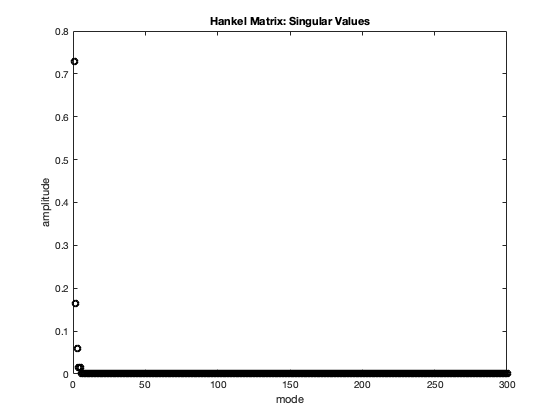
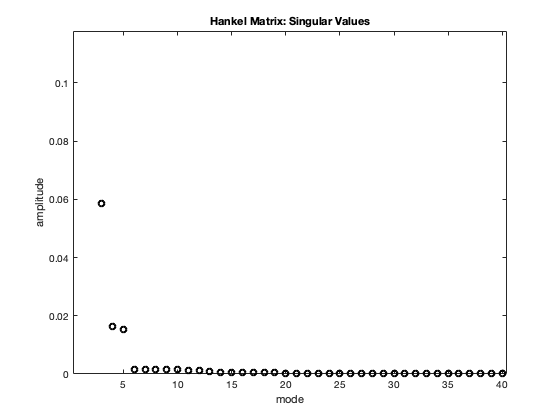
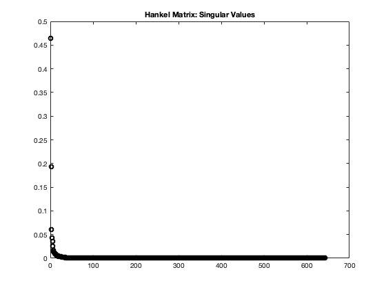
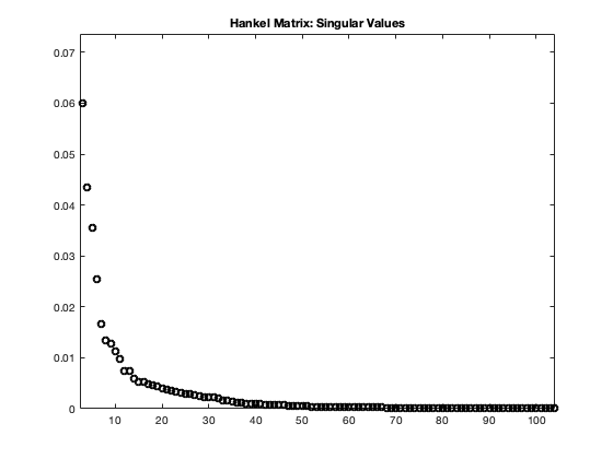
By examining the singular values of the Hankel matrix we can find the best rank- $r$ approximation of the trajectory space. Then, we can form the matrices $\mathbf{X_{1}}$ and $\mathbf{X_{2}}$ for the DMD from $\mathbf{H}$ and set $\ell=r$ for the best DMD approximation using the embedding [3].

3 Algorithm Implementation and Development

We develop the algorithm with the assumption we are given $m$ measurements and $n$ snapshots of a dynamical system with fast and slow scales, but only partial state information. This data forms the matrix $\mathbf{X}\in\mathbb{R}^{m\times n}$ . Since we only have partial state information, the first step in the algorithm is to employ time delay embeddings to form a Hankel matrix $\mathbf{H}$ with $N$ embeddings. We choose an $N$ that minimizes the approximation error in the second stage of the algorithm.

The second step in the algorithm is to form the matrices $\mathbf{X_{1}}$ and $\mathbf{X_{2}}$ from $\mathbf{H}$ , and then apply the DMD method with a rank-reduction that is chosen based on the singular values of $\mathbf{H}$ . This produces the DMD approximation to the dynamical system as given in Equation (6).

The third step in the algorithm is to extract the fast and slow components by applying Equations (8) – (12). These fast and slow components can then be used to form the fast and slow right-hand side functions provided to the ARKODE multirate integrator.

Refer to caption — Figure 1: The time-scale separation algrotihm

4 Computational Results

We applied the time-scale separation algorithm in two different problems. The first problem is a simple, contrived toy problem. The second scenario uses synthetic seismic data for tsunami modeling that is closer to real-world data.

4.1 Toy Problem

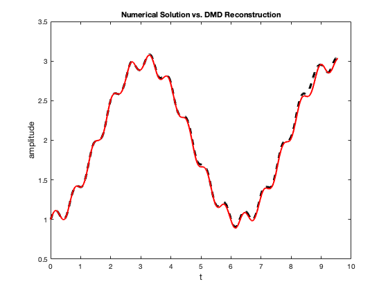
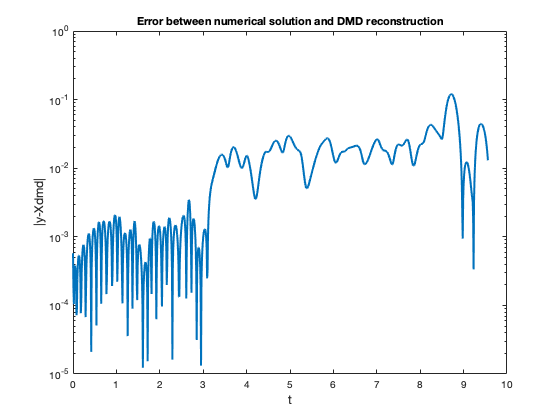
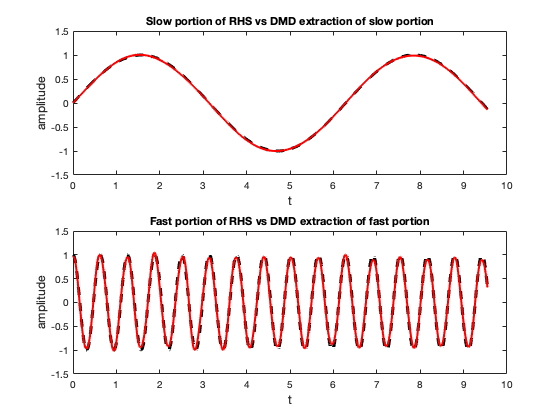
The toy problem uses is defined as the simple IVP:

\frac{dy}{dt}=\cos(10t)+\sin(t),\quad y(0)=1.

It is clear the right hand side has a fast component, $\cos(10t)$ and a slow component $\sin(t)$ . Using MATLAB we solve the ODE with a uniform time step size of 0.01. The solution is used as our dynamics data that we construct the Hankel matrix with and then perform the DMD. The derivative of the fast and slow components extracted is shown in Figure 4. These components were used in the ARKODE solver by reading the different components in from a data file instead of computing the values of the functions at some time instance.

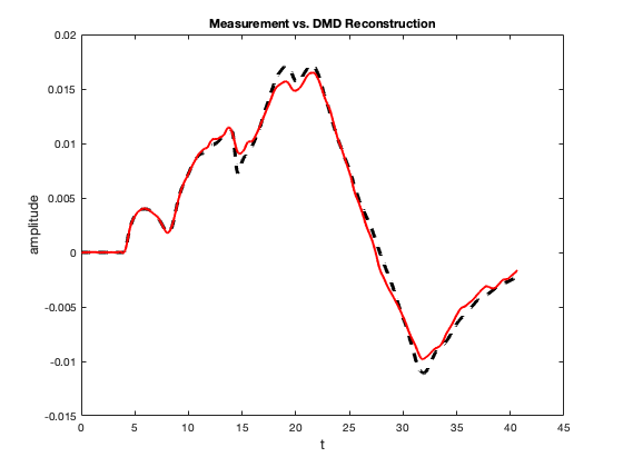
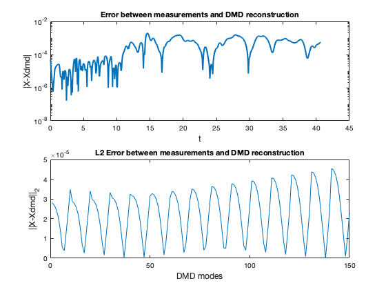
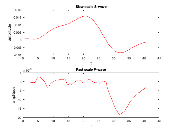
4.2 Synthetic Seismic Data

The second problem we apply our scale separation algorithm to is a seismic problem where waves, or primary waves, are fast and S waves, or secondary waves are slow. In [8], Vogl et al. present a method for a high-resolution seismic model of a fault slippage under the ocean. In the work they present a linear hyperbolic system of equations that model the 2D plane-strain case of isotropic linear elasticity:

q_{t}+A(x,y)q_{x}+B(x,y)q_{y}=0

(14)

A general Riemann solution to produces the eigenvectors of $n_{x}A+n_{y}B$ , where $n=[0~{}~{}1]^{T}$ for the specific data we will examine. The eigenvectors correspond to P and S waves traveling from the source.

As part of their work, Vogl et al. developed a simulation code for the problem based on the Clawpack solver package. The simulation code takes measurements at varying location from the fault with ”gauges”. The data recorded corresponds to the vector $q$ which contains key parameters of the plane-strain equations such as the stress, density and velocity. We build a data matrix $\mathbf{X\in\mathbb{R}^{n\times 10}}$ from 10 sequential gauges and the vertical velocity. This data matrix is then fed into our time scale separation algorithm.

5 Summary and Conclusions

In summary, in this report, we used dynamic mode decomposition and time delay embedding to extract the fast and and slow components of the right-hand sides of a simple ODE from data. We then used the extracted components to solve the ODE with ARKODE. Finally, to move towards a real-world use case, we attempted to extract fast and slow scale dynamics from synthetic seismic modeling data. We found our algorithm to be adequate with the simple dynamics in a toy problem. In the more difficult case with the synthetic seismic data it showed promise, there seemed to be a split of fast and slow scale components, but more work needs to be done to verify the accuracy of the components. In the future, we would like to explore using the multi-resolution DMD presented in [5] to compare the performance and fit for the use case.

6 Acknowledgements

We would like to thank Christopher Vogl for valuable insight into the seismic model used for the synthetic data experiment and with assistance in collecting the data from the simulation code.

This work was performed under the auspices of the U.S. Department of Energy by Lawrence Livermore National Laboratory under Contract DE-AC52-07NA27344. LLNL-TR-848209.

References

[1] D. J. Gardner, D. R. Reynolds, C. S. Woodward, and C. J. Balos, Enabling new flexibility in the sundials suite of nonlinear and differential/algebraic equation solvers, ACM Trans. Math. Softw., 48 (2022).
[2] J. Grosek and J. N. Kutz, Dynamic Mode Decomposition for Real-Time Background/Foreground Separation in Video, arXiv e-prints, (2014), p. arXiv:1404.7592.
[3] M. Kamb, E. Kaiser, S. L. Brunton, and J. N. Kutz, Time-delay observables for koopman: Theory and applications, SIAM Journal on Applied Dynamical Systems, 19 (2020), pp. 886–917.
[4] J. N. Kutz, S. L. Brunton, B. W. Brunton, and J. L. Proctor, Chapter 1: Dynamic Mode Decomposition: An Introduction, 2016, pp. 1–24.
[5] J. N. Kutz, X. Fu, and S. L. Brunton, Multiresolution dynamic mode decomposition, SIAM Journal on Applied Dynamical Systems, 15 (2016), pp. 713–735.
[6] D. R. Reynolds, D. J. Gardner, C. S. Woodward, and R. Chinomona, Arkode: A flexible ivp solver infrastructure for one-step methods, ACM Trans. Math. Softw., (2023). Just Accepted.
[7] J. H. Tu, C. W. Rowley, D. M. Luchtenburg, S. L. Brunton, and J. N. Kutz, On Dynamic Mode Decomposition: Theory and Applications, arXiv e-prints, (2013), p. arXiv:1312.0041.
[8] C. J. Vogl and R. J. LeVeque, A high-resolution finite volume seismic model to generate seafloor deformation for tsunami modeling, Journal of Scientific Computing, 73 (2017), pp. 1204–1215.

Appendix A: MATLAB Code

⬇

function [Phi,omega,lambda,b,Xdyn,Xdmd] = DMD(X1,X2,r,dt)

% function [Phi,omega,lambda,b,Xdmd] = DMD(X1,X2,r,dt) % Computes the Dynamic Mode Decomposition of X1, X2

% INPUTS:

% X1 = X, data matrix

% X2 = X?, shifted data matrix

% Columns of X1 and X2 are state snapshots

% r = target rank of SVD

% dt = time step advancing X1 to X2 (X to X?)

% OUTPUTS:

% Phi, the DMD modes

% omega, the continuous-time DMD eigenvalues

% lambda, the discrete-time DMD eigenvalues

% b, a vector of magnitudes of modes Phi

% Xdmd, the data matrix reconstrcted by Phi, omega, b

%% DMD

[U, S, V] = svd(X1, ’econ’);␣r␣=␣min(r,␣size(U,2));

U_r␣=␣U(:,␣1:r);␣%␣truncate␣to␣rank-r

S_r␣=␣S(1:r,␣1:r);

V_r␣=␣V(:,␣1:r);

Atilde␣=␣U_r’␣*␣X2␣*␣V_r␣/␣S_r;␣%␣low-rank␣dynamics

[W_r,␣D]␣=␣eig(Atilde);

Phi␣=␣X2␣*␣V_r␣/␣S_r␣*␣W_r;␣␣␣␣␣%␣DMD␣modes

lambda␣=␣diag(D);␣␣␣␣␣␣␣␣␣␣␣␣␣␣␣%␣discrete-time␣eigenvalues

omega␣=␣log(lambda)/dt;␣␣␣␣␣␣␣␣␣%␣continuous-time␣eigenvalues

%%␣Compute␣DMD␣mode␣amplitudes␣b

x1␣=␣X1(:,␣1);

b␣=␣Phi\x1;

%%␣DMD␣reconstruction

mm1␣=␣size(X1,␣2);

time_dynamics␣=␣zeros(r,␣mm1);

t␣=␣(0:mm1-1)*dt;␣%␣time␣vector␣for␣iter␣=␣1:mm1,

for␣iter␣=␣1:mm1

␣␣␣␣time_dynamics(:,iter)␣=␣(b.*exp(omega*t(iter)));

end

Xdyn␣=␣time_dynamics;

Xdmd␣=␣Phi␣*␣time_dynamics;

⬇

close all; clear all; clc

fslow=@(t,y) sin(t);

ffast=@(t,y) cos(10*t);

y0=1;

frhs=@(t,y) [ffast(t,y) + fslow(t,y)];

dt=0.01;

tspan=[0:dt:4*pi]; % time span

[t,y]=ode45(@(t,y)frhs(t,y),tspan,y0); % integrate

[~,yslow]=ode45(@(t,y)fslow(t,y),tspan,y0); % integrate

[~,yfast]=ode45(@(t,y)ffast(t,y),tspan,y0); % integrate

% time delay embedding

N=300; % number of embeddings

H=[];

for j=1:N

H=[H; y(j:length(y)-N+j,:).’];

end

[U,S,V]=svd(H,’econ’);␣s=diag(S);

figure(1)

%␣subplot(2,2,[1␣3])

plot(s/sum(s),’ko’,’Linewidth’,2)

title(’Hankel␣Matrix:␣Singular␣Values’)

xlabel(’mode’),␣ylabel(’amplitude’)

%␣subplot(2,2,2)

%␣plot(U(:,1:5))

%␣title(’Modes’)

%␣subplot(2,2,4)

%␣plot(V(:,1:5))

%␣title(’Time’)

%␣DMD␣reconstruction

X1=H(:,1:end-1);␣X2=H(:,2:end);␣tt=t(1:size(X1,2));

[Phi,omega,lambda,b,Xpart,Xdmd]=DMD(X1,X2,25,dt);

error=abs(y(1:length(tt))-Xdmd(1,:)’);

%␣plot

figure(2),␣grid␣on

plot(tt,X1(1,:),’k–’,tt,real(Xdmd(1,:)),’r-’,’Linewidth’,2)

title(’Numerical␣Solution␣vs.␣DMD␣Reconstruction’)

xlabel(’t’,’Fontsize’,12),␣ylabel(’amplitude’,’Fontsize’,12)

figure(3)

semilogy(tt,error,’Linewidth’,2)

title(’Error␣between␣numerical␣solution␣and␣DMD␣reconstruction’)

xlabel(’t’,’Fontsize’,12),␣ylabel(’|y-Xdmd|’,’Fontsize’,12)

%%␣try␣and␣extract␣fast␣and␣slow␣time-scales

w=abs(omega);

eps=0.15;

Xslow=Phi(:,(w/max(w)␣<␣eps))*Xpart((w/max(w)␣<␣eps),:);

%Xfast=Phi(:,(w/max(w)␣>=␣eps))*Xpart((w/max(w)␣>=␣eps),:);

Xfast=Xdmd-abs(Xslow);

figure(4)

subplot(2,1,1)

plot(tt,yslow(1:length(tt)),’k-’,tt,Xslow(1,:),’r-’)

title(’Slow␣scale␣portion␣of␣the␣solution’)

xlabel(’t’,’Fontsize’,12),␣ylabel(’amplitude’,’Fontsize’,12)

subplot(2,1,2)

plot(tt,yfast(1:length(tt)),’k-’,tt,Xfast(1,:)+y0,’r-’)

title(’Fast␣scale␣portion␣of␣the␣solution’)

xlabel(’t’,’Fontsize’,12),␣ylabel(’amplitude’,’Fontsize’,12)

%%␣get␣RHS␣functions␣back␣through␣differentiation

td=tt(1:end-1);

fxslow=diff(Xslow(1,:)’)./diff(tt);

fxfast=diff(Xfast(1,:)’)./diff(tt);

figure(6)

subplot(2,1,1)

plot(td,fslow(td,y0),’k–’,td,fxslow,’r-’,’Linewidth’,2)

title(’Slow␣portion␣of␣RHS␣vs␣DMD␣extraction␣of␣slow␣portion’)

xlabel(’t’,’Fontsize’,12),␣ylabel(’amplitude’,’Fontsize’,12)

subplot(2,1,2)

plot(td,ffast(td,y0),’k–’,td,fxfast,’r-’,’Linewidth’,2)

title(’Fast␣portion␣of␣RHS␣vs␣DMD␣extraction␣of␣fast␣portion’)

xlabel(’t’,’Fontsize’,12),␣ylabel(’amplitude’,’Fontsize’,12)

⬇

clear all; close all; clc

data1 = dlmread(’gauge00030.txt’,”,3,0);

data2␣=␣dlmread(’gauge00031.txt’,”,3,0);

data3␣=␣dlmread(’gauge00032.txt’,”,3,0);

data4␣=␣dlmread(’gauge00033.txt’,”,3,0);

data5␣=␣dlmread(’gauge00034.txt’,”,3,0);

data6␣=␣dlmread(’gauge00035.txt’,”,3,0);

data7␣=␣dlmread(’gauge00036.txt’,”,3,0);

data8␣=␣dlmread(’gauge00037.txt’,”,3,0);

data9␣=␣dlmread(’gauge00038.txt’,”,3,0);

data10␣=␣dlmread(’gauge00039.txt’,”,3,0);

%␣extract␣vertical?␣velocity

j␣=␣7;

t␣=␣data1(:,2);

p␣=␣[data1(:,j),␣data2(:,j),␣data3(:,j),␣data4(:,j),…

␣␣␣␣␣data5(:,j),␣data6(:,j),␣data7(:,j),␣data8(:,j),…

␣␣␣␣␣data9(:,j),␣data10(:,j)];

figure(1)

plot(t,p(:,1),’Linewidth’,2)

%␣V^-1␣qt␣+␣WV^-1␣qx

%%␣time␣delay␣embedding

N=150;␣␣%␣number␣of␣embeddings

H=[];

for␣j=1:N

␣␣H=[H;␣p(j:length(p)-N+j,:).’];

end

[u,sigma,v]␣=␣svd(H,’econ’);␣s␣=␣diag(sigma);

figure(2)

plot(s/sum(s),’ko’,’Linewidth’,2)

title(’Hankel␣Matrix:␣Singular␣Values’)

%␣figure(3)

%␣subplot(2,1,1)

%␣plot(u(:,1:N))

%␣title(’Modes’)

%␣subplot(2,1,2)

%␣plot(v(:,1:N))

%␣title(’Time’)

%%␣DMD␣reconstruction

X1=H(:,1:end-1);␣X2=H(:,2:end);␣dt=t(2)-t(1);␣tt=t(1:size(X1,2));

[Phi,omega,lambda,b,Xdyn,Xdmd]=DMD(X1,X2,75,dt);

error=abs(X1(1,:)-Xdmd(1,:));

l2error=(1/size(X1,2))*sqrt(abs(sum((X1(1:N,:)’-Xdmd(1:N,:)’)).^2));

%␣plot

figure(4),␣grid␣on

plot(tt,X1(1,:),’k–’,tt,real(Xdmd(1,:)),’r-’,’Linewidth’,2)

title(’Measurement␣vs.␣DMD␣Reconstruction’)

xlabel(’t’,’Fontsize’,12),␣ylabel(’amplitude’,’Fontsize’,12)

figure(5)

plot(tt,real(Xdyn),’Linewidth’,2)

title(’DMD␣Dynamics’),␣xlabel(’time’),␣ylabel(’amplitude’)

figure(6)

plot(real(omega),imag(omega),’ko’,’Linewidth’,2)

title(’Eigenvalues’),␣xlabel(’real’),␣ylabel(’imaginary’)

figure(7)

subplot(2,1,1)

semilogy(tt,error,’Linewidth’,2)

title(’Error␣between␣measurements␣and␣DMD␣reconstruction’)

xlabel(’t’,’Fontsize’,12),␣ylabel(’|X-Xdmd|’,’Fontsize’,12)

subplot(2,1,2)

plot(1:N,l2error)

title(’L2␣Error␣between␣measurements␣and␣DMD␣reconstruction’)

xlabel(’DMD␣modes’,’Fontsize’,12),␣ylabel(’||X-Xdmd||_2’,’Fontsize’,12)

%%␣try␣and␣extract␣fast␣and␣slow␣time-scales

w=abs(omega);

eps=0.05;

Xslow=Phi(:,(w/max(w)␣<␣eps))*Xdyn((w/max(w)␣<␣eps),:);

%Xfast=Phi(:,(w/max(w)␣>=␣eps))*Xpart((w/max(w)␣>=␣eps),:);

Xfast=Xdmd-abs(Xslow);

figure(8)

subplot(2,1,1)

plot(tt,real(Xslow(1,:)),’r-’)

title(’Slow␣scale␣S-wave’)

xlabel(’t’,’Fontsize’,12),␣ylabel(’amplitude’,’Fontsize’,12)

subplot(2,1,2)

plot(tt,real(Xfast(1,:)),’r-’)

title(’Fast␣scale␣P-wave’)

xlabel(’t’,’Fontsize’,12),␣ylabel(’amplitude’,’Fontsize’,12)

figure(9),␣plot(tt,real(Xslow(1,:)),’Linewidth’,2)

figure(10),␣plot(tt,real(Xfast(1,:)),’Linewidth’,2)