Data from Model: Extracting Data from Non-robust and Robust Models
Abstract
The essence of deep learning is to exploit data to train a deep neural network (DNN) model. This work explores the reverse process of generating data from a model, attempting to reveal the relationship between the data and the model. We repeat the process of Data to Model (DtM) and Data from Model (DfM) in sequence and explore the loss of feature mapping information by measuring the accuracy drop on the original validation dataset. We perform this experiment for both a non-robust and robust origin model. Our results show that the accuracy drop is limited even after multiple sequences of DtM and DfM, especially for robust models. The success of this cycling transformation can be attributed to the shared feature mapping existing in data and model. Using the same data, we observe that different DtM processes result in models having different features, especially for different network architecture families, even though they achieve comparable performance.
1 Introduction
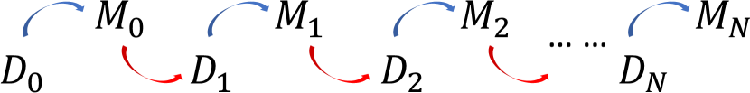
In deep learning applications, such as image classification [6, 18], data is used to train deep neural network (DNN) models. This work explores the reverse process of generating data from the model, with one general question in mind: What is the relationship between data and model? This question cannot be addressed well by only focusing on the model training process, Data To Model (DtM) [8]. Thus we combine the widely adopted DtM with its reverse process of Data from Model (DfM). More specifically, we repeat the process of DtM and DfM in sequence and measure the accuracy over the original validation dataset. In this chaining process, we always assume access to only either the data or the model generated in the previous process. More specifically, in the DtM process, we can only access the data generated from the previous DfM process, and similarly, in the DfM process, we only access the model generated by the previous DtM process. This chain process is depicted in Figure 1.
Our work is mainly inspired by [7] which attributes the success of adversarial examples to the existence of non-robust features (mappings) in a dataset. During the typical DtM process, these non-robust features are learned by a model which consequently has the same non-robust features. This indicates the feature mapping as the link between data and model. In their work, the original training dataset is adopted as the background image in the data extraction process [7]. In this work, we explore the possibility of retrieving a learned feature mapping from a trained model without the original training dataset, which makes the DfM process more meaningful. Moreover, we iterate the DtM and DfM process in sequence instead of just performing it once. Another aspect of this work is to explore whether such feature mappings are the same or different for different runs for the same or different architectures.
To decode the learned features of a model into a dataset without knowledge of the original training data, we adopt random substitute datasets as background to increase sample diversity and introduce virtual logits to model the logit behavior of DNNs. Our experiments show that we can obtain models with similar properties as the original model in terms of both accuracy and robustness. We showcase the effectiveness of our approach on MNIST and CIFAR10 for both non-robust and robust origin models.
2 Related Work
DNNs are vulnerable to small, imperceptible perturbations [13]. This intriguing phenomenon led to various attack [4, 2, 9, 11, 16] and defense methods [3]. Interpretations for the reason of the existence of adversarial examples have been explored in [4, 14, 17]. Ilyas et al. [7] attributed the phenomenon of adversarial examples to the existence of non-robust features. They introduce features as a mapping relationship from the input to the output. We adopt this definition and aim to extract this feature mapping from the model to the data. Model visualization methods [12, 10] can be seen as a DfM method, without training a new model on the extracted data. Such methods are commonly further exploited for model compression [5, 1] techniques. Instead of compressing models, [15] aims to compress an entire dataset into only a few synthetic images. Training on these few synthetic images, however, leads to a serious performance drop.
3 Methodology
Given a -classification dataset consisting of data samples and their corresponding true class , a DNN ( omitted from now on) parameterized through the weights is commonly trained via mini-batch stochastic gradient descent (SGD) to achieve . In this work, we term this process DtM (data to model) and we explore its reverse process of extracting data from model (DfM). More specifically, starting from origin dataset DtM results in origin model , with DfM, can be extracted which leads to through DtM and so on. During the DtM and DfM process, we assume having no access to the previous models and datasets, respectively.
To retrieve features from a model and store them in the form of data, we deploy the -variant of projected gradient descent (PGD) [9]. Due to the absence of the original dataset, we leverage substitute images from a substitute dataset , as well as virtual logits as the target values for the gradient-based optimization process. We specify the logit output of a classifier as and use the -loss between the network output logit and the virtual target logit as the loss function optimized by PGD. The retrieved dataset consists of images , where indicates a vector optimized through PGD and lies in the range . The data samples and their respective output logit values represent the new dataset.
After the DfM process, the retrieved dataset can be used in the DtM process, by training the model weights with the -distance between the previously stored ground truth logit vector and the output logit vector, .
We heuristically found a simple scheme of Gaussian distributed values for the virtual logits. The highest logit is determined by , and the mean values of the remaining logit values are equally separated between with . The order of logit values is chosen randomly to introduce diversity into the dataset.
In the above process, the origin model is non-robust. Following [7] we also use a robust model for obtained with adversarial training and repeat the chaining process.
4 Experiments
4.1 DfM and DtM in sequence
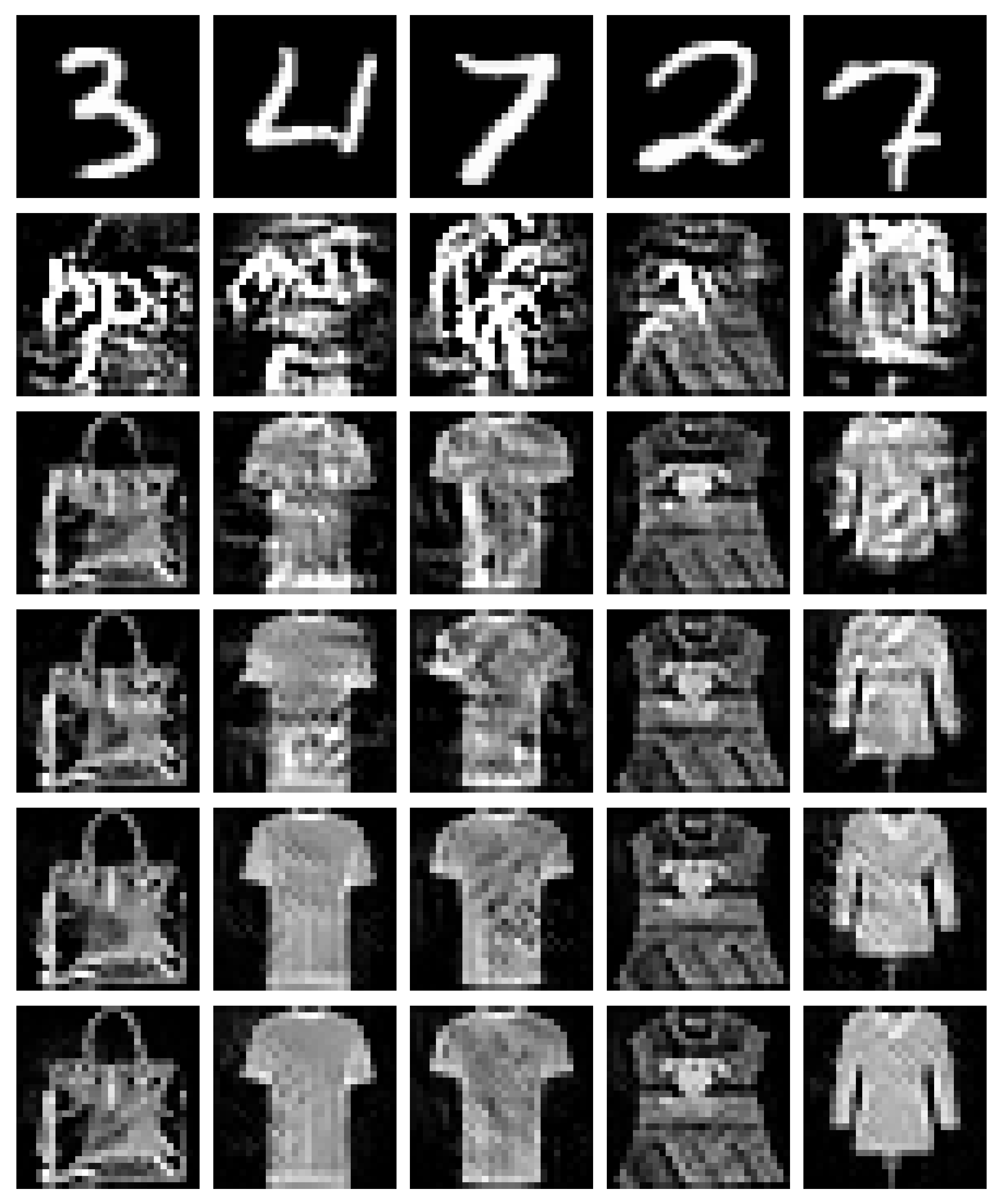
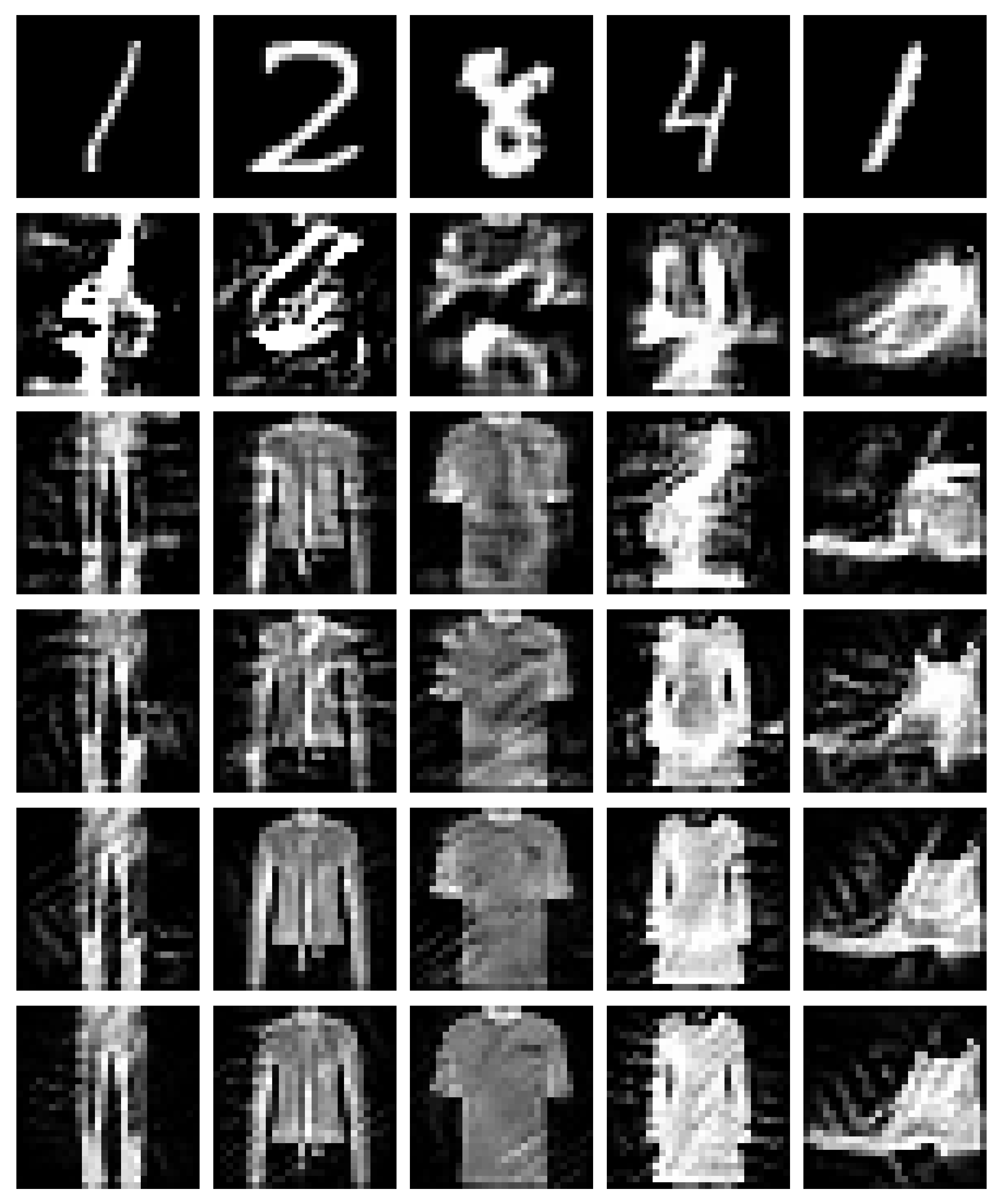
We sequentially apply DfM and DtM starting from the origin model . The non-robust and robust origin models are obtained through standard and adversarial training, respectively, on LeNet for MNIST and VGG8 for CIFAR10. VGG8 refers to a VGG network with only one convolution layer between each max pooling operation. To obtain from the preceding model , k images are extracted from through the DfM process. For the background images, we choose Fashion MNIST and MS-COCO as background images for MNIST and CIFAR10, respectively. The generated images are shown in Figure 2. In subsequent DtM, dataset is then used to train the model which is an independent model of the same architecture. The accuracy for all models is reported on the original validation dataset. We present the results with five repetitions of this process in Table 1.
| LeNet (MNIST) | VGG8 (CIFAR10) | |||
|---|---|---|---|---|
| non-robust | robust | non-robust | robust | |
| non-robust | robust | |||||||||
|---|---|---|---|---|---|---|---|---|---|---|
Qualitative results in Figure 2 show that the extracted images look totally different from the original images, due to which it might be tempting to expect the models trained on them will work poorly on the original validation dataset. Table 1, however, shows that comparable performance is achieved and this is due to similar feature mappings existing in the generated images despite the large visual discrepancy. Nonetheless, we observe that there is a general trend that the accuracies for both the non-robust and robust models decrease for each sequence of DfM/DtM. The accuracy increase by from to for the robust VGG8 model is the only exception to this. For the non-robust origin model , the accuracy drop is trivial in the first few iterations of the DfM and DtM process and it becomes more observable in later iterations. For the robust origin model , the accuracy is retained better. For example, the robust LeNet only decreases by from to , while the non-robust LeNet decreases by .
We further investigate the robustness to adversarial examples for the models from the DfM/DtM process. Therefore we evaluate the different retrieved MNIST models on adversarial examples generated with -PGD under different , update steps and the corresponding step size calculated as . Similar to the observed accuracy drop for clean images, a similar trend occurs when the model is under attack. However, the accuracy degradation seems to be more severe for robustness. For example, the accuracy of the non-robust LeNet drops from to for a relatively weak attack of while the clean image accuracy drops from to . Similar behavior is observed for the models originating from the robust . It is worth mentioning that the models originating from the robust are consistently more robust than their counterparts originating from the non-robust . After two subsequent DfM iterations starting from the robust , still shows similar robustness as the standard non-robust model . This result suggests that DfM can be applied as an alternative to adversarial training.
4.2 DfM and DtM on different architectures
| VGG16 | VGG19 | ResNet18 | ResNet50 | ||
|---|---|---|---|---|---|
| non-rob. | VGG16 () | ||||
| VGG19 () | |||||
| ResNet18 () | |||||
| robust | VGG16 () | ||||
| VGG19 () | |||||
| ResNet18 () |
The above analysis shows that DtM and DfM can be performed for the same and simple architecture with a limited performance drop. Here we apply DfM to the standard and adversarially trained CIFAR10 models and train different state-of-the-art architectures on the extracted data. For simplicity we stop the chaining process after obtaining . The results in Table 3 show that all model architectures can be successfully trained on the extracted data. Similar to Table 1, a performance drop is observed for the data extracted from the non-robust . For the robust , however, we observe that the retrained consistently outperforms their corresponding for both similar and different architectures, which is somewhat surprising.
4.3 Do different models learn different feature mappings?
| VGG16 | VGG19 | ResNet18 | ResNet50 | ||
|---|---|---|---|---|---|
| non-robust | VGG16 | ||||
| VGG19 | |||||
| ResNet18 | |||||
| ResNet50 | |||||
| robust | VGG16 | ||||
| VGG19 | |||||
| ResNet18 | |||||
| ResNet50 |
Given the possibility to extract a certain feature mapping from a model, in this section, we analyze whether different models trained from the same origin dataset have different feature mappings. To this end, we utilize k feature images extracted from models trained under the same conditions, and perform a cross-evaluation of the model accuracy on each other. The results for models with standard and adversarial training are reported in Table 4. We observe that the cross-evaluation accuracies are higher than random guess, which indicates that some shared feature mappings are learned. However, for both non-robust and robust models only in a few cases an accuracy higher than is achieved. This phenomenon can also be observed when the extracted dataset was evaluated on an independently trained instance of the same architecture as the original architecture. The relatively low cross-evaluation accuracies illustrate that models from different runs learn different features which are not fully compatible with each other.
Another interesting observation is that model architectures from the same network family, VGG family for instance, seem to have more common feature mappings than different architectures. For example, for the feature images extracted from the standard ResNet50, the ResNet networks exhibit an accuracy of around , while the VGG networks only show an accuracy of around . This phenomenon is more prevalent in non-robust models than in robust models. Overall, the results show that different models learn different feature mappings from the same dataset even though they have comparable classification accuracy.
5 Conclusion
In this work we introduced the Data from Model (DfM) process, a technique to reverse the conventional model training process, by extracting data back from the model. A model trained on the generated dataset that look totally different from the original dataset can achieve comparable performance as their counterparts trained on the origin dataset. The success of this technique confirmed feature mapping as the link between data and model. Our work provides insight about the relationship between data and model as well understanding of model robustness.
References
- [1] Kartikeya Bhardwaj, Naveen Suda, and Radu Marculescu. Dream distillation: A data-independent model compression framework. arXiv preprint arXiv:1905.07072, 2019.
- [2] Nicholas Carlini and David Wagner. Towards evaluating the robustness of neural networks. In Symposium on Security and Privacy (SP), 2017.
- [3] Anirban Chakraborty, Manaar Alam, Vishal Dey, Anupam Chattopadhyay, and Debdeep Mukhopadhyay. Adversarial attacks and defences: A survey. arXiv preprint arXiv:1810.00069, 2018.
- [4] Ian J Goodfellow, Jonathon Shlens, and Christian Szegedy. Explaining and harnessing adversarial examples. In International Conference on Learning Representations (ICLR), 2015.
- [5] Matan Haroush, Itay Hubara, Elad Hoffer, and Daniel Soudry. The knowledge within: Methods for data-free model compression. arXiv preprint arXiv:1912.01274, 2019.
- [6] Kaiming He, Xiangyu Zhang, Shaoqing Ren, and Jian Sun. Identity mappings in deep residual networks. In European Conference on Computer Vision (ECCV), 2016.
- [7] Andrew Ilyas, Shibani Santurkar, Dimitris Tsipras, Logan Engstrom, Brandon Tran, and Aleksander Madry. Adversarial examples are not bugs, they are features. In Advances in Neural Information Processing Systems (NeurIPS), 2019.
- [8] Alex Krizhevsky, Ilya Sutskever, and Geoffrey E Hinton. Imagenet classification with deep convolutional neural networks. In Advances in Neural Information Processing Systems (NeurIPS), 2012.
- [9] Aleksander Madry, Aleksandar Makelov, Ludwig Schmidt, Dimitris Tsipras, and Adrian Vladu. Towards deep learning models resistant to adversarial attacks. In International Conference on Learning Representations (ICLR), 2018.
- [10] Aravindh Mahendran and Andrea Vedaldi. Understanding deep image representations by inverting them. In Conference on Computer Vision and Pattern Recognition (CVPR), 2015.
- [11] Seyed-Mohsen Moosavi-Dezfooli, Alhussein Fawzi, Omar Fawzi, and Pascal Frossard. Universal adversarial perturbations. In Conference on Computer Vision and Pattern Recognition (CVPR), 2017.
- [12] Alexander Mordvintsev, Christopher Olah, and Mike Tyka. Inceptionism: Going deeper into neural networks. 2015.
- [13] Christian Szegedy, Wojciech Zaremba, Ilya Sutskever, Joan Bruna, Dumitru Erhan, Ian Goodfellow, and Rob Fergus. Intriguing properties of neural networks. arXiv preprint arXiv:1312.6199, 2013.
- [14] Thomas Tanay and Lewis Griffin. A boundary tilting persepective on the phenomenon of adversarial examples. arXiv preprint arXiv:1608.07690, 2016.
- [15] Tongzhou Wang, Jun-Yan Zhu, Antonio Torralba, and Alexei A Efros. Dataset distillation. arXiv preprint arXiv:1811.10959, 2018.
- [16] Chaoning Zhang, Philipp Benz, Tooba Imtiaz, and In-So Kweon. Cd-uap: Class discriminative universal adversarial perturbation. In AAAI Conference on Artificial Intelligence (AAAI), 2020.
- [17] Chaoning Zhang, Philipp Benz, Tooba Imtiaz, and In-So Kweon. Understanding adversarial examples from the mutual influence of images and perturbations. In Conference on Computer Vision and Pattern Recognition (CVPR), 2020.
- [18] Chaoning Zhang, Francois Rameau, Seokju Lee, Junsik Kim, Philipp Benz, Dawit Mureja Argaw, Jean-Charles Bazin, and In So Kweon. Revisiting residual networks with nonlinear shortcuts. In British Machine Vision Conference (BMVC), 2019.