Data-fusion using factor analysis and low-rank matrix completion
Abstract
Data-fusion involves the integration of multiple related datasets. The statistical file-matching problem is a canonical data-fusion problem in multivariate analysis, where the objective is to characterise the joint distribution of a set of variables when only strict subsets of marginal distributions have been observed. Estimation of the covariance matrix of the full set of variables is challenging given the missing-data pattern. Factor analysis models use lower-dimensional latent variables in the data-generating process, and this introduces low-rank components in the complete-data matrix and the population covariance matrix. The low-rank structure of the factor analysis model can be exploited to estimate the full covariance matrix from incomplete data via low-rank matrix completion. We prove the identifiability of the factor analysis model in the statistical file-matching problem under conditions on the number of factors and the number of shared variables over the observed marginal subsets. Additionally, we provide an EM algorithm for parameter estimation. On several real datasets, the factor model gives smaller reconstruction errors in file-matching problems than the common approaches for low-rank matrix completion.
1 Introduction
Data-fusion involves the joint modelling of multiple related datasets, with the aim to lift the quality of inference that could be obtained from isolated separate analyses of each dataset. The statistical file-matching problem is a classic data-fusion task, where all observations are from the same population, with the caveat that different sets of variables are recorded in each individual dataset (Little and Rubin, 2002; Rässler, 2002; D’Orazio et al., 2006a). The core problem can be reduced to the analysis of two datasets, labelled A and B, with three groups of variables denoted , and . Dataset A contains observations on the variables and Dataset B contains observations on the variables. Table 1 describes the missing-data pattern. The statistical file-matching problem occurs in bioinformatics such as in flow cytomtery analysis in the synthesis of multiplexed data collected using different panels of markers (Pedreira et al., 2008; Lee et al., 2011; O’Neill et al., 2015; Abdelaal et al., 2019). Other important application areas include survey sampling and data integration in official statistics (Conti et al., 2016; D’Orazio, 2019).
| Variables | |||
|---|---|---|---|
| Dataset A | observed | observed | — |
| Dataset B | observed | — | observed |
We assume that dataset A and dataset B are samples from the same homogeneous population. For example, in flow cytometry analysis a single blood sample from a patient may be divided into two aliquots which are then analysed using markers and respectively. Technological limitations prevent joint measurements on the and markers. In survey sampling, one random subset of the population may receive a questionnaire with items and a second random subset of the population given items . This situation may arise when integrating results from related surveys, or in the design of a single survey where there is a constraint on the response burden.
Key linear relationships between , and are encoded in the covariance matrix :
| (1) |
A fundamental task in the statistical file-matching problem is the estimation of from incomplete data (Rässler, 2002; D’Orazio et al., 2006a). A common objective in file-matching is to impute the missing observations so that complete-data techniques can be used in downstream tasks. Recovery of is crucial to generating proper imputations (Little, 1988; Van Buuren, 2018). The covariance matrix is also important for Gaussian graphical modelling, and the recovery of a network model from incomplete information is an interesting problem (Sachs et al., 2009).
The critical issue in the statistical file-matching problem is how to estimate without any joint observations on the and variables. Factor analysis models are useful in data-fusion tasks as they provide structured covariance matrices that allow the sharing of information across variables (Li and Jung, 2017; O’Connell and Lock, 2019; Park and Lock, 2020). In the statistical file-matching problem, this can facilitate the estimation of from the observed and associations. Let , and denote the dimensions of , , and respectively, with . A factor analysis model consists of a matrix of factor loadings and a diagonal matrix of uniqueness terms, giving the structured covariance matrix . The full covariance matrix can be written as
| (2) |
where and have been partitioned as
where is a matrix of factor loadings for the variables, and is a diagonal matrix of uniquenesses for the variables. The and parameters are partitioned in a similar fashion. Assuming that and can be recovered from the observed blocks of the covariance matrix, it is possible to learn as .
The file-matching problem can be approached as a low-rank matrix completion task. One may attempt to complete the partial estimate of the covariance matrix or to complete the partially observed data matrix. Generic results for matrix recovery with random missingness patterns do not give clear guidance on the feasibility of statistical file-matching with the fixed and systematic missing-data pattern in Table 1 (Candes and Plan, 2010).
We provide conditions for the identifiability of the factor analysis model given the missing-data pattern in the file-matching problem. The main result is that recovery of is possible if the number of latent factors satisfies , and (Theorem 1). Additionally, we give an EM algorithm (Dempster et al., 1977) for joint estimation of and with closed form E- and M-steps. We find that on several real datasets, maximum likelihood factor analysis gives better estimates of than common existing approaches for low-rank matrix completion.
2 Methods
Here we review some existing approaches that can be used to estimate in the statistical file-matching problem.
2.1 Conditional independence assumption
A common resolution to the identifiability issue in the file-matching problem is to assume that and are conditionally independent given . Under this assumption, . The conditional independence assumption is commonly invoked to justify statistical matching (D’Orazio et al., 2006a; Rässler, 2002). However, it is untestable and can have a large influence on downstream results (Barry, 1988; Rodgers, 1984).
2.2 Identified set
To avoid making assumptions, the generative model can be treated as being partially identified (Gustafson, 2015). There is a growing literature focused on developing uncertainty bounds for the matching problem that reflect the limited information in the sample (D’Orazio et al., 2006b; Conti et al., 2012, 2016). For the multivariate normal model, the goal is to estimate the a feasible set of values for , rather than to deliver a point estimate (Kadane, 2001; Moriarity and Scheuren, 2001; Ahfock et al., 2016). The restriction that the covariance matrix be positive definite creates an identified set
| (3) |
A disadvantage of the partial identification approach is that the level of uncertainty on can be very high. Bounds on the parameters can be too wide for any practical interpretation.
2.3 Low-rank matrix completion
Low-rank matrix completion may be applied to fill in the partial estimate of the covariance matrix or to impute the missing observations in the partially observed data matrix. To complete the estimate of the covariance matrix , one may consider the regularised least-squares objective
where is the nuclear norm of the matrix (Candes and Plan, 2010; Mazumder et al., 2010) and contains the indices of the known elements of . The main barrier to attempting matrix completion on is that the presence of the diagonal matrix along with the symmetry constraint on necessitates modifications to existing algorithms for low-rank matrix completion. The algorithm for symmetric low-rank matrix completion with block missingness developed in Bishop and Byron (2014) could be a useful starting point.
A more natural approach in the file-matching problem is to use a low-rank matrix completion algorithm to impute the missing data. Partitioning the complete-dataset as
where the first row corresponds to dataset A, and the second row corresponds to dataset B, the missing and observations can be estimated by applying matrix completion to . The modelling assumption is that complete-dataset can be expressed as for some rank matrix plus noise . To estimate , the following least squares objective can be used
where is a matrix, is a matrix and contains the indices of the observed elements in . With , the low-rank estimate of is
| (4) |
Using the low-rank reconstructions and as imputed values for the missing-data and , an estimate of is then given by
The theoretical work in Koltchinskii et al. (2011) can be used to give finite-sample bounds on the reconstruction error under assumptions on the noise matrix . However, in the context of the file-matching problem, it is not immediately clear from existing theoretical work whether exact recovery of the true covariance is possible in the large-sample limit.
3 Factor models for statistical file-matching
3.1 Generative model
A probabilistic factor analysis model with factors has the latent variable representation
| (5) |
where , , and
Kamakura and Wedel (2000) discuss the application of factor analysis models to the statistical file-matching problem, but do not consider the identifiability of the model, or develop an algorithm for parameter estimation. We address both of these important points. We prove the identifiability of the factor analysis model in the file-matching problem under the following assumptions.
Assumption 1.
The matrix of factors for the variables, , is of rank .
Assumption 2.
Define
For both and , if any row is removed, there remain two disjoint submatrices of rank .
3.2 Identifiability
The key to recovery of is that the matrix is of rank . Lemma 1 shows that it is possible to complete the matrix given the missing-data pattern in Table 1.
Lemma 1.
Suppose that Assumption 1 is satisfied. If all blocks other than and of
are observed, then it is possible to recover from the observed elements. Consider the eigenvalue decomposition of the two sub-blocks of that are relevant to dataset A and dataset B:
The factors for the marginal models for dataset A and dataset B in the canonical rotation are
To recover from the observed elements set
where , and and are the left and right singular vectors of the matrix .
The proof is given in the Appendix. Bishop and Byron (2014) establish more general results for the low-rank completion of symmetric matrices with structured missingness. Although Lemma 1 is sufficient for low-rank matrix completion problems, identifiability of the factor analysis model is a more complex issue. Specifically, for two parameter sets and , the equality does not imply that (Anderson and Rubin, 1956; Shapiro, 1985). Assumption 2 allows us to make a statement about the identifiability of the factor analysis model in the file-matching problem.
Theorem 1.
The proof is given in the Appendix. In terms of the generative model in Section 3.1, Theorem 1 states that if parameter sets and satisfy and then the factor loadings in and are equal up to post-multiplication on the right by an orthogonal matrix. The conclusion is that recovery of in the file-matching scenario is possible given the observable sub-blocks of the population covariance matrix . Assuming that the sample covariance matrices converge in probability to the population quantities as , consistent estimation of is possible.
Under mild regularity conditions on the factor loadings, is sufficient for identifiability of the factor analysis model with complete-cases (Anderson and Rubin, 1956; Shapiro, 1985). In the file-matching scenario, Assumption 2 enforces the stronger condition that and . If the number of factors falls within the intervals and , Assumption 2 is violated. However, one may hope that the model is still identifiable, given that consistent estimation is possible with complete-cases.
Some insight can be gained by comparing the number of equations and the number of unknowns (Ledermann, 1937). There are unknown parameters in and unknown parameters in . Given the symmetry in , there are equations, and the adoption of a rotation constraint on yields an additional equations (Anderson and Rubin, 1956). The number of equations minus the number of unknowns is . A useful rule of thumb is to expect the the factor analysis model to be identifiable if , and nonidentifiable if (Ledermann, 1937; Anderson and Rubin, 1956). Bekker and ten Berge (1997) show that is sufficient for the identifiability of the factor model in most circumstances. In the file-matching problem, the equality constraints due to are not present and the degrees of freedom is now reduced to . If is negative and is positive it may signal a situation where the missing-data has caused the factor model to be nonidentifiable.
Table 2 reports the maximum number of allowable factors using the degrees of freedom criteria and , and the restrictions of Assumption 2 in a file-matching problem with . Assumption 2 places stronger requirements on the number of factors than the degrees of freedom requirement . The number of allowable factors using is smaller than , demonstrating the information loss due to the missing-data.
| Criterion | Quantity | 3 | 6 | 9 | 12 | 15 | 18 | 21 |
|---|---|---|---|---|---|---|---|---|
| Degrees of freedom, complete-cases | 1 | 3 | 5 | 7 | 10 | 12 | 15 | |
| Degrees of freedom, file-matching | 0 | 2 | 3 | 5 | 6 | 8 | 9 | |
| Assumption 2 | 0 | 1 | 2 | 3 | 4 | 5 | 6 | |
3.3 Estimation
As mentioned in Section 2.3, procedures for low-rank matrix completion focus on the estimation of rather than the joint estimation of and . A maximum likelihood approach to the factor analysis model facilitates joint estimation of and . With complete-cases, the EM updates for factor analysis can be written in closed form (Rubin and Thayer, 1982). Let denote the sample scatter matrix
| (8) |
Given current parameter estimates of and , define . The M-step is
| (9) | ||||
| (10) |
For the file-matching problem we need to compute the conditional expectation of (8) given the missing-data pattern. The observed scatter matrices in dataset A and dataset B are
| (11) | ||||
| (12) |
To determine the conditional expectation of the complete-data sufficient statistic, for current parameter estimates of and define
and the conditional covariance matrices
Using the augmented scatter matrices
the expected value of the complete-data sufficient statistic is given by
Given current parameter estimates of , define . The M-step is then
| (13) | ||||
| (14) |
The EM algorithm can be run using the sample covariance matrices from dataset A and dataset B, and so it is not necessary to have the original observations. The multivariate normality assumption used to develop the algorithm is not crucial, as long as the population covariance matrix fits the factor analysis model (Browne, 1984).
3.4 Model selection
In practice, the number of factors must be determined. The Bayesian information criterion (Schwarz, 1978) is a generic tool for model selection that has been well explored in factor analysis for selecting (Preacher et al., 2013). The Bayesian information criterion for a model with likelihood function and parameter is given by
| (15) |
where is the maximum likelihood estimate, is the number of free parameters in the model , and is the sample size (Schwarz, 1978). For factor analysis with complete-cases the log-likelihood is
where and is the sample scatter matrix (8). The Bayesian information criterion for factor analysis with complete-cases is therefore
where the number of free parameters is obtained by subracting the number of rotation constraints from the nominal number of parameters .
For model selection in missing-data problems it has been suggested to use the observed-data log-likelihood in place of the complete-data log-likelihood in the standard definition of the Bayesian information criterion (15) (Ibrahim et al., 2008). This is the strategy we propose to use for determining the number of factors in the file-matching problem. The log-likelihood functions for each dataset are given by
where , , is the observed scatter matrix from dataset A (11), is the observed scatter matrix from dataset B (12) and
The Bayesian information criterion using the observed-data log-likelihood is then
4 Simulation
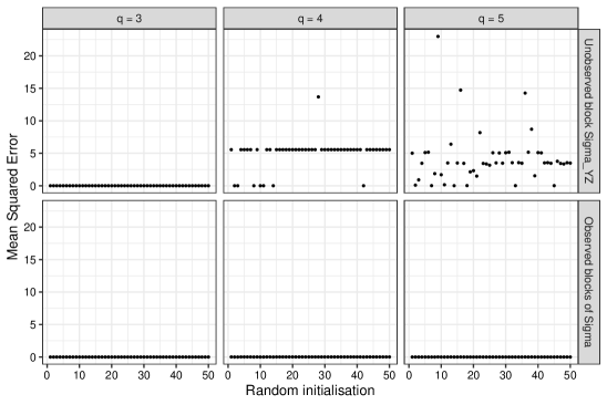
Here we investigate the necessity of Assumption 2 for the identifiability of the factor model by focusing on the noiseless setting where the exact covariance matrix is known with the exception of . We considered a file-matching scenario with . As seen in Table 2, Assumption 2 enforces stricter requirements than the degrees of freedom criterion based on . We simulated three different covariance matrices with , one from a factor model, one from a factor model, and one from a factor model. Elements of were sampled from a distribution. The th diagonal element of was set as , where . Assumption 2 holds only for , but the degrees of freedom is non-negative for .
For each covariance matrix, we fit a factor model using the EM algorithm for 10000 iterations using a random initial value , where each element was sampled from a distribution. The correct number of factors was used for each of the three test matrices. Given the estimate , we computed the mean squared error over the elements of , that is . We also computed the mean squared error for the observed blocks of . This procedure was repeated fifty times. Figure 1 displays the results over the fifty random initialisations for each of the three covariance matrices .
The top row shows the estimation errors for , the bottom row shows the estimation errors for the observed blocks of . Looking at the bottom row, for , and the EM algorithm is able to reconstruct the observed blocks of over each random initialisation. From the top row, for , the choice of initial values does not affect the final estimate of , and the estimation error is zero in each trial. For and , the choice of initial values influences the final estimate of . As the reconstruction error for the observed blocks of is zero, this suggests there are multiple factor solutions and the model is not identifiable. The divergent behaviour when comparing to and is notable, as Assumption 2 is only satisfied for . The degrees of freedom are non-negative for and , but this does not lead to a well-behaved estimator. In this simulation, Assumption 2 appears to give better guidelines for the stable recovery of compared to .
5 Data application
5.1 Estimation
In this section we compare the performance of various algorithms for the estimation of . Existing algorithms for low-rank matrix completion were implemented using the R package filling (You, 2020). We also considered the standard conditional independence assumption (CIA). We tested the algorithms on the following datasets.
-
•
Sachs dataset. This dataset consists of results from 11 flow cytometry experiments measuring the same set of 12 variables. The measurements were log transformed. Data from each experiment was centered, then combined and scaled so that each variable had unit variance.
-
•
Wisconsin breast cancer dataset. The original observations in the malignant class were centered and scaled so that each variable had unit variance.
-
•
Abalone dataset. The original observations in the female class were centered and scaled so that each variable had unit variance.
For each dataset we considered matching scenarios with common variables, unique variables in dataset A, and unique variables in dataset B. This defines partitions of the complete-dataset. Table 3 gives the file-matching scenarios considered for each dataset, as well as the number of factors that were used in the fitting of the factor analysis model. The final columns indicate whether the degrees of freedom criteria and , and Assumption 2 are satisfied for the chosen number of factors . Assumption 2 is violated on the Sachs dataset, but the degrees of freedom is positive.
| Dataset | Assumption 2 | |||||||
|---|---|---|---|---|---|---|---|---|
| Sachs | 11 | 4 | 4 | 3 | 4 | Yes | Yes | No |
| Wisconsin | 10 | 3 | 3 | 4 | 2 | Yes | Yes | Yes |
| Abalone | 8 | 1 | 4 | 3 | 1 | Yes | Yes | Yes |
In each simulation, variables were randomly allocated to the , , and groups. We then used different algorithms to estimate . The mean squared error over elements of was then recorded for each algorithm, that is . This process was repeated 100 times. The EM algorithm was run for 2000 iterations in each simulation. We considered two different initial value settings for the EM algorithm, initialisation using the factor analysis solution from the full covariance matrix, and random initialisation of by sampling from a standard normal distribution. For the random initialisation protocol we took one hundred samples of followed by a short run of the EM algorithm for fifty iterations. The parameters with the highest log-likelihood after the fifty iterations were then used in the longer run. In each simulation we also fit a factor model using the complete-dataset with no missing data to provide a reference point for the goodness-of-fit of the factor model.
Figure 2 compares the results using the different algorithms. The results for factor analysis model with the favourable initial values are shown as FM, the results for the factor analysis model with random initialisation are shown as FM (random). The factor model with good initial values (FM) has the lowest median error across each dataset (Table 4). The errors on the Sachs dataset and the Wisconsin breast cancer dataset are particularly small.
The results for the factor model with random initialisation (FM (random)) are very similar to those of FM using the favourable initial values except on the Sachs dataset. On the Sachs dataset, Assumption 2 is violated and there may be multiple factor solutions. In Figure 2 (a), the errors for the factor model with random initialisation (FM (random)) are much more dispersed than the factor model with the good initial values (FM). Although there are sufficient degrees of freedom , it appears that the model may not be identifiable. With good initial values, the EM algorithm appears to converge to a local mode that gives a good estimate of .
The interquartile range of the error for each algorithm over the one hundred variable permutations is given in Table 4. The factor analysis model (FM) has the smallest interquartile range on each dataset, closely followed by the factor model using random initialisations with the exception of the Sachs dataset.

| Dataset | Value | FM | CIA | Soft-Impute | SVD | FM (random) | Complete |
|---|---|---|---|---|---|---|---|
| Sachs | Median | 0.0006 | 0.0320 | 0.0465 | 3.1174 | 0.0402 | 0.0001 |
| IQR | 0.0017 | 0.0351 | 0.0518 | 27.822 | 0.0907 | 0.0001 | |
| Wisconsin | Median | 0.0032 | 0.0125 | 0.0058 | 0.0059 | 0.0036 | 0.0006 |
| IQR | 0.0023 | 0.0216 | 0.0073 | 0.0113 | 0.0025 | 0.0008 | |
| Abalone | Median | 0.0042 | 0.0125 | 0.0089 | 0.0102 | 0.0042 | 0.0031 |
| IQR | 0.0031 | 0.0198 | 0.0081 | 0.0142 | 0.0031 | 0.0024 |
5.2 Model selection
We also performed some experiments to assess the behavior of the Bayesian information criterion for determining the number of factors . The following datasets and variable partitions were used in the experiments
-
•
Reise dataset. This dataset is a correlation matrix for mental health items. The variables were partitioned as , and .
-
•
Harman dataset. This dataset is a correlation matrix for psychological tests. The variables were partitioned as , and .
-
•
Holzinger dataset. This dataset is a correlation matrix for mental ability scores. The variables were partitioned as , and .
-
•
Simulated from a factor model with and . Elements of were sampled from a distribution. The th diagonal element of was set as , where . The covariance matrix was then standardised to a correlation matrix. We simulated one dataset with observations and one dataset of observations. The variables were partitioned as .
In each simulation, variables were randomly allocated to the , and groups with . We then computed the BIC for a range of values for and recorded the optimal value . This process was repeated 100 times. In each of the simulations we considered the range of values for such that Assumptions 1 and 2 were satisfied. Table 5 reports the number of times a factor model was chosen using the BIC over the 100 replications. The optimal number of factors according to the BIC using complete-cases is given as in Table 5. The missing-data appears to lead to the BIC acting conservatively, selecting a number of factors less than or equal to the number chosen with complete-cases. The correct number of factors is selected for the simulated datasets when using complete-cases. For the simulated dataset with , the BIC selects fewer than six factors in each trial. For the simulated dataset with the BIC selects the correct number of factors in each replication. Figure 3 shows boxplots of the estimation error for different values of . The errors from using the conditional independence assumption and from fitting a factor model with complete-cases are also reported for comparison. For almost all values of , the median error using the factor model is lower than that of the conditional independence model.
| Dataset | |||||||||
|---|---|---|---|---|---|---|---|---|---|
| Reise | 8 | 0 | 1 | 1 | 18 | 80 | - | - | - |
| Harman | 3 | 62 | 37 | 1 | 0 | 0 | - | - | - |
| Holzinger | 4 | 0 | 60 | 37 | 3 | - | - | - | - |
| Simulated | 6 | 5 | 51 | 41 | 3 | 0 | 0 | 0 | 0 |
| Simulated | 6 | 0 | 0 | 0 | 0 | 0 | 100 | 0 | 0 |

6 Discussion
Technological and design constraints can prevent investigators from collecting a full dataset on all variables of interest. The statistical file-matching problem is an important data-fusion task where joint observations on the full set of variables are not available. Factor analysis models are useful as they can remain identifiable despite the missing-data pattern of the file-matching problem. The factor analysis approach is a useful alternative to the conditional independence assumption, as it is less restrictive and testable. Estimation of the factor analysis model can be carried out via the EM algorithm.
Although factor analysis and low-rank matrix completion are related, the identifiability of the factor analysis model requires additional assumptions compared to low-rank matrix completion due to the diagonal matrix . As the assumption that and may be unnecessarily strong, it is of interest to establish the weakest conditions that ensure the identifiability of the factor analysis model in the file-matching problem. In many applications of file-matching, procedures for generating uncertainty bounds when the model is partially identified supply useful information (Conti et al., 2016). Further work may explore characterisations of the identified set for the factor analysis model when the number of latent factors exceeds the maximum number for identifiability.
It is also of interest to relax the assumption that both datasets are samples from the same homogeneous population with the joint model . One possible avenue is to embed the file-matching problem in a hierarchical model. A dataset specific random effect can be applied to the parameters in dataset A and dataset B, so that there is shared component across datasets and a unique component within each dataset. Samples in dataset A are from the distribution , and samples from dataset B are from the distribution where and where and are random effect terms. The added flexibility of the hierarchical model can allow for situations where datasets A and B are from related but not necessarily identical populations, a common scenario in data integration. Model identifiability with heterogeneous data sources is an interesting and challenging problem, and the results here may serve as useful groundwork.
Acknowledgements
This research was funded by the Australian Government through the Australian Research Council (Project Numbers DP170100907 and IC170100035).
References
- Abdelaal et al. (2019) Abdelaal, T., Höllt, T., van Unen, V., Lelieveldt, B. P. F., Koning, F., Reinders, M. J. T. and Mahfouz, A. (2019) CyTOFmerge: integrating mass cytometry data across multiple panels. Bioinformatics, 35, 4063–4071.
- Ahfock et al. (2016) Ahfock, D., Pyne, S., Lee, S. X. and McLachlan, G. J. (2016) Partial identification in the statistical matching problem. Computational Statistics and Data Analysis, 104, 79–90.
- Anderson and Rubin (1956) Anderson, T. W. and Rubin, H. (1956) Statistical inference in factor analysis. In Proceedings of the Third Berkeley Symposium on Mathematical Statistics and Probability, 238–246.
- Barry (1988) Barry, J. T. (1988) An investigation of statistical matching. Journal of Applied Statistics, 15, 275–283.
- Bekker and ten Berge (1997) Bekker, P. A. and ten Berge, J. M. (1997) Generic global identification in factor analysis. Linear Algebra and its Applications, 264, 255 – 263.
- Bishop and Byron (2014) Bishop, W. E. and Byron, M. Y. (2014) Deterministic symmetric positive semidefinite matrix completion. In Advances in Neural Information Processing Systems, 2762–2770.
- Browne (1984) Browne, M. W. (1984) Asymptotically distribution-free methods for the analysis of covariance structures. British Journal of Mathematical and Statistical Psychology, 37, 62–83.
- Candes and Plan (2010) Candes, E. J. and Plan, Y. (2010) Matrix completion with noise. Proceedings of the IEEE, 98, 925–936.
- Conti et al. (2012) Conti, P. L., Marella, D. and Scanu, M. (2012) Uncertainty analysis in statistical matching. Journal of Official Statistics, 28, 69–88.
- Conti et al. (2016) — (2016) Statistical matching analysis for complex survey data with applications. Journal of the American Statistical Association, 111, 1715–1725.
- Dempster et al. (1977) Dempster, A. P., Laird, N. M. and Rubin, D. B. (1977) Maximum likelihood from incomplete data via the EM algorithm (with discussion). Journal of the Royal Statistical Society B, 39, 1–38.
- D’Orazio (2019) D’Orazio, M. (2019) Statistical learning in official statistics: The case of statistical matching. Statistical Journal of the IAOS, 35, 435–441.
- D’Orazio et al. (2006a) D’Orazio, M., Di Zio, M. and Scanu, M. (2006a) Statistical Matching: Theory and Practice. New York: Wiley.
- D’Orazio et al. (2006b) D’Orazio, M., Zio, M. and Scanu, M. (2006b) Statistical matching for categorical data: Displaying uncertainty and using logical constraints. Journal of Official Statistics, 22, 137.
- Gustafson (2015) Gustafson, P. (2015) Bayesian Inference for Partially Identified Models: Exploring the Limits of Limited Data. Boca Raton: CRC Press.
- Ibrahim et al. (2008) Ibrahim, J. G., Zhu, H. and Tang, N. (2008) Model selection criteria for missing-data problems using the EM algorithm. Journal of the American Statistical Association, 103, 1648–1658.
- Kadane (2001) Kadane, J. B. (2001) Some statistical problems in merging data files. Journal of Official Statistics, 17, 423.
- Kamakura and Wedel (2000) Kamakura, W. A. and Wedel, M. (2000) Factor analysis and missing data. Journal of Marketing Research, 37, 490–498.
- Koltchinskii et al. (2011) Koltchinskii, V., Lounici, K. and Tsybakov, A. B. (2011) Nuclear-norm penalization and optimal rates for noisy low-rank matrix completion. Annals of Statistics, 39, 2302–2329.
- Ledermann (1937) Ledermann, W. (1937) On the rank of the reduced correlational matrix in multiple-factor analysis. Psychometrika, 2, 85–93.
- Lee et al. (2011) Lee, G., Finn, W. and Scott, C. (2011) Statistical file matching of flow cytometry data. Journal of Biomedical Informatics, 44, 663–676.
- Li and Jung (2017) Li, G. and Jung, S. (2017) Incorporating covariates into integrated factor analysis of multi-view data. Biometrics, 73, 1433–1442.
- Little (1988) Little, R. J. (1988) Missing-data adjustments in large surveys. Journal of Business & Economic Statistics, 6, 287–296.
- Little and Rubin (2002) Little, R. J. A. and Rubin, D. B. (2002) Statistical Analysis with Missing Data. Hoboken: Wiley, 2nd edn.
- Mazumder et al. (2010) Mazumder, R., Hastie, T. and Tibshirani, R. (2010) Spectral regularization algorithms for learning large incomplete matrices. The Journal of Machine Learning Research, 11, 2287–2322.
- Moriarity and Scheuren (2001) Moriarity, C. and Scheuren, F. (2001) Statistical matching: a paradigm for assessing the uncertainty in the procedure. Journal of Official Statistics, 17, 407.
- O’Connell and Lock (2019) O’Connell, M. J. and Lock, E. F. (2019) Linked matrix factorization. Biometrics, 75, 582–592.
- O’Neill et al. (2015) O’Neill, K., Aghaeepour, N., Parker, J., Hogge, D., Karsan, A., Dalal, B. and Brinkman, R. R. (2015) Deep profiling of multitube flow cytometry data. Bioinformatics, 31, 1623–1631.
- Park and Lock (2020) Park, J. Y. and Lock, E. F. (2020) Integrative factorization of bidimensionally linked matrices. Biometrics, 76, 61–74.
- Pedreira et al. (2008) Pedreira, C. E., Costa, E. S., Barrena, S., Lecrevisse, Q., Almeida, J., van Dongen, J. J. M. and Orfao, A. (2008) Generation of flow cytometry data files with a potentially infinite number of dimensions. Cytometry Part A, 73, 834–846.
- Preacher et al. (2013) Preacher, K. J., Zhang, G., Kim, C. and Mels, G. (2013) Choosing the optimal number of factors in exploratory factor analysis: A model selection perspective. Multivariate Behavioral Research, 48, 28–56.
- Rässler (2002) Rässler, S. (2002) Statistical Matching: A Frequentist Theory, Practical Applications, and Alternative Bayesian Approaches. New York: Springer-Verlag.
- Rodgers (1984) Rodgers, W. L. (1984) An Evaluation of Statistical Matching. Journal of Business & Economic Statistics, 2, 91.
- Rubin and Thayer (1982) Rubin, D. B. and Thayer, D. T. (1982) EM algorithms for ML factor analysis. Psychometrika, 47, 69–76.
- Sachs et al. (2009) Sachs, K., Itani, S., Carlisle, J., Nolan, G. P., Pe’er, D. and Lauffenburger, D. A. (2009) Learning signaling network structures with sparsely distributed data. Journal of Computational Biology, 16, 201–212.
- Schönemann (1966) Schönemann, P. H. (1966) A generalized solution of the orthogonal Procrustes problem. Psychometrika, 31, 1–10.
- Schwarz (1978) Schwarz, G. (1978) Estimating the dimension of a model. Annals of Statistics, 6, 461–464.
- Shapiro (1985) Shapiro, A. (1985) Identifiability of factor analysis: Some results and open problems. Linear Algebra and its Applications, 70, 1–7.
- Van Buuren (2018) Van Buuren, S. (2018) Flexible Imputation of Missing Data. Boca Raton: CRC Press.
- You (2020) You, K. (2020) filling: Matrix Completion, Imputation, and Inpainting Methods. R package version 0.2.1.
Appendix A Appendix
A.1 Proof of Lemma 1
Due to the rotational invariance of the factor model, we have that
| (A.1) |
for orthogonal matrices , and . The alignment of and is an orthogonal Procrustes problem. Let be the solution to the optimisation problem
| (A.2) |
Assuming that and are of full column rank, Schönemann (1966) showed that there is a unique solution to (A.2). As , both and are of rank under Assumption 1. Define and let the singular value decomposition of be given by . Then using the result from Schönemann (1966), the unique solution to (A.2) is given by . The uniqueness of the solution implies that as from (A.1). Then again using (A.1). Finally, .
A.2 Proof of Theorem 1
Using Theorem 5.1 in Anderson and Rubin (1956), Assumption 2 guarantees that if
then the uniquenesses are equal, , , and , implying
| (A.3) | ||||
| (A.4) |
Using Lemma 1, can be uniquely recovered given the matrices on the left-hand side of (A.3) and (A.4). Likewise, can be uniquely recovered given the matrices on the right hand side of (A.3) and (A.4). It remains to show that . To do so, define the eigendecompositions
and the rotated and scaled eigenvectors
Using Assumption 1 and Lemma 1, the equality
| (A.5) |
must hold, where and are the left and right singular vectors of the matrix . Combining the equalities in (A.3), (A.4) and (A.5) gives the main result