Decentralized Federated Averaging
Abstract
Federated averaging (FedAvg) is a communication efficient algorithm for the distributed training with an enormous number of clients. In FedAvg, clients keep their data locally for privacy protection; a central parameter server is used to communicate between clients. This central server distributes the parameters to each client and collects the updated parameters from clients. FedAvg is mostly studied in centralized fashions, which requires massive communication between server and clients in each communication. Moreover, attacking the central server can break the whole system’s privacy. In this paper, we study the decentralized FedAvg with momentum (DFedAvgM), which is implemented on clients that are connected by an undirected graph. In DFedAvgM, all clients perform stochastic gradient descent with momentum and communicate with their neighbors only. To further reduce the communication cost, we also consider the quantized DFedAvgM. We prove convergence of the (quantized) DFedAvgM under trivial assumptions; the convergence rate can be improved when the loss function satisfies the PŁ property. Finally, we numerically verify the efficacy of DFedAvgM.
Index Terms:
Decentralized Optimization, Federated Averaging, Momentum, Stochastic Gradient Descent1 Introduction
Federated learning (FL) is a privacy-preserving distributed machine learning (ML) paradigm [1]. In FL, a central server connects with enormous clients (e.g., mobile phones, pad, etc.); the clients keep their data without sharing it with the server. In each communication round, clients receive the current global model from the server, and a small portion of clients are selected to update the global model by running stochastic gradient descent (SGD) [2] for multiple iterations using local data. The central server then aggregates these updated parameters to obtain the updated global model. The above learning algorithm is known as federated average (FedAvg) [1]. In particular, if the clients are homogeneous, FedAvg is equivalent to the local SGD [3]. FedAvg involves multiple local SGD updates and one aggregation by the server in each communication round, which significantly reduces the communication cost between sever and clients compared to the conventional distributed training with one local SGD update and one communication.
In FL applications, large companies and government organizations usually play the role of the central server. On the one hand, since the number of clients in FL is massive, the communication cost between the server and clients can be a bottleneck [4]. On the other hand, the updated models collected from clients encode the private information of the local data; hackers can attack the central server to break the privacy of the whole system, which remains the privacy issue as a serious concern. To this end, decentralized federated learning has been proposed [5, 6], where all clients are connected with an undirected graph. Decentralized FL replaces the server-clients communication in FL with clients-clients communication.
In this paper, we consider two issues about decentralized FL: 1) Although there is no expensive communication between server and clients in decentralized FL, the communication between local clients is costly when the ML model itself is large. Therefore, it is crucial to ask can we reduce the communication cost between clients? 2) Momentum is a well-known acceleration technique for SGD [7]. It is natural to ask can we use SGD with momentum to improve the training of ML models in decentralized FL with theoretical convergence guarantees?
1.1 Our Contributions
We answer the above questions affirmatively by proposing the decentralized FedAvg with momentum (DFedAvgM). To further reduce the communication cost between clients, we also integrate quantization with DFedAvgM. Our contributions in this paper are elaborated below in threefold.
-
•
Algorithmically, we extend FedAvg to the decentralized setting, where all clients are connected by an undirected graph. We motivate DFedAvgM from the decentralized SGD (DSGD) algorithm. In particular, we use SGD with momentum to train ML models on each client. To reduce the communication cost between each client, we further introduce a quantized version of DFedAvgM, in which each client will send and receive a quantized model.
-
•
Theoretically, we prove the convergence of (quantized) DFedAvgM. Our theoretical results show that the convergence rate of (quantized) DFedAvgM is not inferior to that of SGD or DSGD. More specifically, we show that the convergence rates of both DFedAvgM and quantized DFedAvgM depend on the local training and the graph that connects all clients. Besides the convergence results under nonconvex assumptions, we also establish their convergence guarantee under the Polyak-Łojasiewicz (PŁ) condition, which has been widely studied in nonconvex optimization. Under the PŁ condition, we establish a faster convergence rate for (quantized) DFedAvgM. Furthermore, we present a sufficient condition to guarantee reducing communication costs.
-
•
Empirically, we perform extensive numerical experiments on training deep neural networks (DNNs) on various datasets in both IID and Non-IID settings. Our results show the effectiveness of (quantized) DFedAvgM for training ML models, saving communication costs, and protecting training data’s membership privacy.
1.2 More Related Works
We briefly review three lines of work that are most related to this paper, i.e., federated learning, decentralized training, and decentralized federated learning.
Federated Learning. Many variants of FedAvg have been developed with theoretical guarantees. [8] uses the momentum method for local clients in FedAvg. [9] proposes the adaptive FedAvg, whose central parameter server uses the adaptive learning rate ti aggregate local models. Lazy and quantizatized gradients are used to reduce communications [10, 11]. [12] proposes a Newton-type scheme for FL. The convergence analysis of FedAvg on heterogeneous data is discussed by [13, 14]. The advances and open problems in FL is available in two survey papers [15, 16].
Decentralized Training. Decentralized algorithms are originally developed to calculate the mean of data that are distributed over multiple sensors [17, 18, 19, 20]. Decentralized (sub)gradient descents (DGD), one of the simplest and efficient decentralized algorithms, have been studied in [21, 22, 23, 24, 25]. In DGD, the convexity assumption is unnecessary [26], which makes DGD useful for nonconvex optimization. A provably convergent DSGD is proposed in [27, 28, 4]. [27] provides the complexity result of a stochastic decentralized algorithm. [28] designs a stochastic decentralized algorithm with the dual information and provide the theoretical convergence guarantee. [4] proves that DSGD outperforms SGD in communication efficiency. Asynchronous DSGD is analyzed in [29]. DGD with momentum is proposed in [30, 31]. Quantized DSGD has been proposed in [32].
Decentralized Federated Learning. Decentralized FL is a learning paradigm of choice when the edge devices do not trust the central server in protecting their privacy [33]. The authors in [34] propose a novel FL framework without a central server for medical applications, and the new method offers a highly dynamic peer-to-peer environment. [6] considers training an ML model with a connected network whose nodes take a Bayesian-like approach by introducing a belief of the parameter space.
1.3 Organizations
We organize this paper as follows: in section 2, we present a mathematical formulation of our problem and some necessary assumption. In section 3, we present the DFedAvgM and its quantized algorithms. We present the convergence of the proposed algorithm in section 4. We provide extensive numerical verification of DFedAvgM in section 6. This paper ends up with concluding remarks. Technical proofs and more experimental details are provided in the appendix.
1.4 Notation
We denote scalars and vectors by lower case and lower case boldface letters, respectively, and matrices by upper case boldface letters. For a vector , we denote its norm () by , and denote the norm of by and denote norm as . For a matrix , we denote its transpose as . Given two sequences and , we write if there exists a positive constant such that , and we write if there exist two positive constants and such that and . hides the logarithmic factor of . For a function , we denote its gradient as and its Hessian as , and denote its minimum as . We use to denote the expectation with respect to the underlying probability space.
2 Problem Formulation and Assumptions
We consider the following optimization task
| (1) |
where denotes the data distribution in the -th client and is the loss function associated with the training data . Problem (1) models many applications in ML, which is known as empirical risk minimization (ERM). We list several assumptions for the subsequent analysis.
Assumption 1
The function is differentiable and is -Lipschitz continuous, , i.e., for all .
The first-order Lipschitz assumption is commonly used in the ML community. Here, for simplicity, we suppose all functions enjoy the same Lipschitz constant . We can also assume that these functions have non-uniform Lipschitz constants, which does not affect our convergent analysis.
Assumption 2
The gradient of the function have -bounded variance, i.e., for all . This paper also assumes the (global) variance is bounded, i.e., for all .
The uniform local variance assumption is also used for the ease of presentation, which is straightforward to generalize to non-uniform cases. The global variance assumption is used in [9, 35]. The constant reflects the heterogeneity of the data sets , and when follow the same distribution, .
An important notion in decentralized optimization is the mixing matrix, which is usually associated with a connected graph with the vertex set and the edge set . Any edge represents a communication link between nodes and . We recall the definition of the mixing matrix associated with the graph .
Definition 1 (Mixing matrix)
The mixing matrix is assumed to have the following properties: 1. (Graph) If and , then , otherwise, ; 2. (Symmetry) ; 3. (Null space property) ; 4. (Spectral property)
For a graph, the corresponding mixing matrix is not unique; given the adjacency matrix of a graph, its maximum-degree matrix and metropolis-hastings [37] are both mixing matrices. The symmetric property of indicates that its eigenvalues are real and can be sorted in the non-increasing order. Let denote the -th largest eigenvalue of , that is, 111This is based on the spectral property of mixing matrix. The mixing matrix also serves as a probability transition matrix of a Markov chain. A quite important constant of is , which describes the speed of the Markov chain introduced by the mixing matrix converges to the stable state.
3 Decentralized Federated Averaging
3.1 Decentralized FedAvg with Momentum
We first briefly review the previous work on decentralized training, which carries out in the following fashion:
-
1.
client holds an approximate copy of the parameters and calculate an unbiased estimate of at . can be non-consensus;
-
2.
(communication) client updates its local parameters as the weighted average of its neighbors: ;
-
3.
(training) client updates its parameters as with a learning rate .
The traditional decentralization can be described in Figure 1 (a), in which, a communication step is needed after each training iteration. This indicate that the above vanilla decentralized algorithm is different from FedAvg, and the later performs multiple local training step before communication. To this end, we have to slightly modify the scheme of the decentralized algorithm. For simplicity, we consider modifying DSGD to motivate our decentralized FedAvg algorithm. Note that when the original DGD is applied to solve (1), we end up with the following iteration
| (2) | ||||
where we used the fact that . In (2), if we replace by , the algorithm then iterates as
| (3) |
In (3), clients communicate with their neighbors after one training iteration, which is then possible to generalize to the federated optimization setting. We replace the single SGD iteration in (3) with multiple SGD with heavy-ball [38] iterations. Therefore, the DFedAvgM can be presented as follows: In each , for each client , let . The inner iteration in each node then performs as
| (4) |
where . After inner iterations in each local client, the resulting parameters is sent to its neighbors (). Every client then updates its parameters by taking the local averaging as follows
| (5) |
The procedure of DFedAvgM can be illustrated as Figure 1 (b). It is seen that DFedAvgM plays the tradeoff between local computing and communications. It is well-known that the communication costs are usually much more expensive than the computation costs [39], which indicates DFedAvgM can be more efficient than DSGD.
3.2 Efficient Communication via Quantization
In DFedAvgM, client needs to send to its neighbours . Thus, when the number of neighbours grows, client-client communications become the major bottleneck on algorithms’ efficiency. We leverage the quantization trick to reduce the communication cost [40, 41]. In particular, we consider the following quantization procedure: Given a constant and the limited bit number , the representable range is then . For any with , we can find an integer such that and we then use to replace . The above quantization scheme is deterministic, which can be written as for ; Besides the deterministic rule, the stochastic quantization uses the following scheme
It is easy to see that the stochastic quantization is unbiased, i.e., for any . When is small, deterministic and stochastic quantization schemes perform very similarly. For a vector whose coordinates are all stored with bits, we consider quantizing all coordinates of . The multi-dimension quantization operator is then defined as
| (6) |
For both deterministic and stochastic quantization schemes, we have if for . In this paper, we consider a quantization operator with the following assumption, which hold for the two quantization schemes mentioned above.
Assumption 4
The quantization operator satisfies with for any .
Directly quantize the parameters is feasible for sufficiently smooth loss functions, but may be impossible for DNNs. To this end, we consider quantizing the difference the difference of parameters. Quantized DFedAvgM can be summarized as: After running (4) times, client quantizes and send it to . After receiving , every client updates its local parameters as
| (7) |
In each communication, client just needs to send the pair to , whose representation requires bits rather than bits for sending the unquantized version. If is large and , the communications can be significantly reduced.
4 Convergence Analysis
In this section, we analyze the convergence of the proposed (quantized) DFedAvgM. The convergence analysis of DFedAvgM is much more complicated than SGD, SGD with momentum, and DSGD; the technical difficulty is because fails to be an unbiased estimate of the gradient after multiple iterations of SGD or SGD with momentum in each client. In the following, we consider the convergence of the average point, which is defined as . We first present the convergence of DFedAvgM for general nonconvex objective function in the following Theorem.
Theorem 1 (General nonconvexity)
Let the sequence be generated by DFedAvgM for and suppose Assumptions 1, 2 and 3 hold. Moreover, assume the stepsize for SGD with momentum that used for training client models satisfies
where is the Lipschitz constant of and is the number of client iterations before each communication. Then
where is the total number of communication rounds and the constants are given as
and
To get an explicit rate on from Theorem 1, we choose . As is large enough and . Then, , and , and . Based on this choice of and the Theorem 1, we have the following convergence rate for DFedAvgM.
Proposition 1
As the communication round number is large enough, it holds that
From Proposition 1, we can see that the speed of DFedAvgM can be improved when the number of local iteration, , increases. Also, when the momentum is and is large enough, the bound will be dominated by , in which the local variance bound diminishes. This phenomenon coincides with our intuitive understanding: in local client, the use of large can result in a local minimizer; then the local variance bound will hurt nothing. To reach any given error, DFedAvgM needs communication rounds, which is the same as SGD and DSGD. It is worth mentioning that the above theoretical results show that whether the momentum can accelerate the algorithm depends on the relation between and , i.e., if , as increases, the rate improves; if , large may degrade the performance of DFedAvgM.
The convergence results established above, which simply require smooth assumption on the objective functions, are quite general and somehow not sharp due to extra properties are missing. For example, recent (non)convex studies [42, 43, 44] have exploited the algorithmic performance under the PŁ property, which is named after Polyak and Łojasiewicz [45, 46]. For a smooth function , we say it satisfies PŁ- property provided
| (8) |
The well-known strong convexity implies PŁ condition, but not vice verse. In the following, we present the convergence of DFedAvgM under the PŁ condition.
Theorem 2 (PŁ condition)
Assume function satisfies the PŁ- condition, the following convergence rate holds
Due to the fact that , the right side is larger than . If we still let , the convergence rate is at least . But we cannot choose a very small ; otherwise, the dominated term will decay very slowly. If the learning rate enjoys the form as with 222This learning rate is commonly used in the ML community., we can prove the following results on the optimal choices for .
Proposition 2
Let with , the optimal rate of DFedAvgM is , in which case , , and , that is, .
This finding coincides with existing results of the optimal rate for SGD with strong convexity [47, 48]. Under the PŁ condition, the convergence rate of DFedAvgM is improved.
Next, we provide the convergence guarantee for the quantized DFedAvgM, which is stated in the following theorem.
Theorem 3
Let the sequence be generated by the quantized DFedAvgM for all , and all the assumptions in Theorem 1 and Assumption 4 hold. Let , as is sufficiently large, it holds that
If the function further satisfies the PŁ condition and , it follows that
According to Theorem 3, to reach any given error in general case, we need to set and set the the number of communication round as . While with PŁ condition, we set and . It follows Therefore, under the PŁ condition, the number of communication round is reduced.
In the following, we provide a sufficient condition for communications-saving of the two quantization rules mentioned in Sec. 3.2 used in quantized DFedAvgM.
Proposition 3
Assume we use the stochastic or deterministic quantization rule with bits using stepsize . Assume that the parameters trained in all clients do not overflow, that is, all coordinates are contained in . Let Assumptions 1, 2 and 3 hold. If the desired error
and , the quantized DFedAvgM can beat DFedAvgM with 32 bits in term of the required communications to reach .
Proposition 3 indicates that the superiority of the quantized DFedAvgM retains when the desired error is not smaller than . We can also see that as increases, the guaranteed lower bound of decreases, which demonstrates the necessity of multiple local iterations. Moreover, a larger can also reduce the lower bound.
5 Proofs
5.1 Technical Lemmas
We define and
For a matrix , we denote its spectral norm as . We also define .
Lemma 1
In [Proposition 1, [21]], the author also proved that for some that depends on the matrix.
Lemma 2
Assume that Assumptions 2 and 3 hold, and . Let be generated by the (quantized) DFedAvgM. It then follows
when .
Lemma 3
Given the stepsize and and assume , are generated by the (quantized) DFedAvgM for all . If Assumption 3 holds, it then follows
where when .
With the fact that , Lemma 3 also holds for .
Lemma 4
Given the stepsize and let be generated by DFedAvgM for all . If Assumption 3 holds, we have the following bound
| (9) |
where .
Lemma 5
Given the stepsize and assume are generated by the quantized DFedAvgM for all . If Assumption 3 holds, it follows that
| (10) |
5.2 Proof of Technical Lemmas
5.2.1 Proof of Lemma 2
Given any , the Cauchy inequality gives us
where uses the Cauchy’s inequality with and . Without loss of generality, we assume . Let , we get
Using the mathematical induction, for any integer , we have
5.2.2 Proof of Lemma 3
Note that for any , in node it holds
where and . The unbiased expectation property of gives us
| I | |||
On the other hand, with Lemma 2, we have the following bound
Thus, we can obtain
where the last inequality depends on the selection of the stepsize. The recursion from to yeilds
where we used the inequality holds for any .
5.2.3 Proof of Lemma 4
We denote . With these notation, we have
| (11) |
where . The iteration (11) can be rewritten as the following expression
| (12) |
Obviously, it follows
| (13) |
According to Lemma 1, it holds
Multiplying both sides of (12) with and using (13), we then get
| (14) |
where we used initialization . Then, we are led to
| (15) | ||||
With Cauchy inequality,
Direct calculation gives us
With Lemma 3 and Assumption 3, for any ,
Thus, we get
The fact that then proves the result.
5.2.4 Proof of Lemma 5
5.3 Proof of Theorem 1
Noting that , that is also
we have
| (17) |
where . With the local scheme in each node,
Thus, we get
| (18) | ||||
The Lipschitz continuity of gives us
| (19) |
where we used (17). Let
we can derive
where uses (18). Similarly, we can get
Thus, (5.3) can be represented as
Direct computation together with Lemma 4 gives us
Therefore, we have
| (20) | ||||
Summing the inequality (20) from to , we then proved the result.
5.4 Proof of Theorem 2
With the PŁ condition,
We start from (20),
| (21) | ||||
By defining , it then follows
| (22) | ||||
Thus, we are then led to
The result is then proved.
5.5 Proof of Proposition 2
A quick calculation gives us
Thus, we just need to bound the first term in Theorem 2. As is large, . Its logarithm is then
With our setting, it follows
Then we have
We first consider how to choose . From the L’Hospital’s rule, for any , as
Thus, we need to set and the fast rate is slower than . To this end, we choose , , and .
5.6 Proof of Theorem 3
Let , in the quantized DFedAvgM, it follows With the Lipschitz continuity of ,
We have
and
Note that both and can inherit the bounds of and in the proof of Theorem 1. Thus, we obtain
With Lemma 5, we can get
Combining the inequalities together,
where Given the stepsize , we can see that as is large. When is small, . And it then follows . We now consider
| (23) | ||||
which is at the order as . If the function satisfies the PŁ-, we have
When , and
5.7 Proof of Proposition 3
We calculate to reach the same error, the communication costs by both algorithms. Omitting the order larger than 1 for , from (20), we have
for DFedAvgM. From (23),
Given the , assume obeys
That means DFedAvgM can output an error in iterations. However, due to the error caused by the quantization, we have to increase the iteration number for quantized DFedAvgM. We set the iteration number as . To get the error for quantized DFedAvgM, we also need , which yields
The total communication cost of DFedAvgM to reach is
While for quantized version, the total communication cost is
Thus, the communications can be reduced if
6 Numerical Results
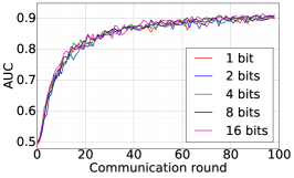
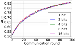
We apply the proposed DFedAvgM with communication quantization to train DNNs for both image classification and language modeling, where we consider a simple ring structured communication network. We aim to verify that DFedAvgM can train DNNs effectively, especially in communication efficiency. Moreover, we consider the membership privacy protection when DFedAvgM is used for training DNNs. We apply the membership inference attack (MIA) [49] to test the efficiency of (quantized) DFedAvgM in protecting the training data’s MP. In MIA, the attack model is a binary classifier 333We use a multilayer perceptron with a hidden layer of 64 nodes, followed by a softmax output function as the attack model, which is adapted from [49]., which is to decide if a data point is in the training set of the target model. For each of the following dataset, to perform MIA we first split its training set into and with the same size. Furthermore, we split into two halves with the same size and denote them as and , and we split by half into and . MIA proceeds as follows: 1) train the shadow model by using ; 2) apply the trained shadow model to predict all data points in and train the corresponding classification probabilities of belonging to each class. Then we take the top three classification probabilities (or two in the case of binary classification) to form the feature vector for each data point.A feature vector is tagged as1if the corresponding data point is in , and otherwise. Then we train the attack model by leveraging all the labeled feature vectors; 3) train the target model by using and obtain feature vector for each point in . Finally, we leverage the attack model to decide if a data point is in . Note the attack model we build is a binary classifier, which is to decide if a data point is in the training set of the target model. For any data , we apply the attack model to predict its probability () of belonging to the training set of the target model. Given any fixed threshold if , we classify as a member of the training set (positive sample), and if , we conclude that is not in the training set (negative sample); so we can obtain different attack results with different thresholds. We can plot the ROC curve for different threshold, and regard the area under the ROC curve (AUC) as an evaluation of the membership inference attack.The target model protects perfect membership privacy if the AUC is 0.5 (attack model performs random guess), and the higher AUC is, the less private the target model is.
6.1 MNIST Classification
The efficiency of DFedAvgM.
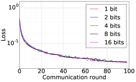
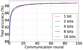
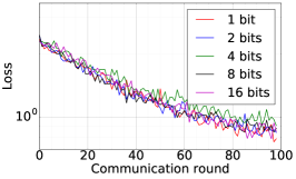
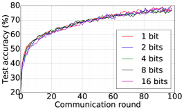
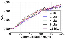
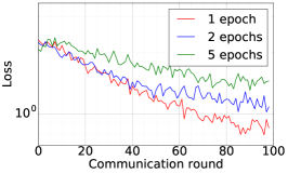
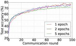
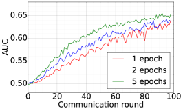
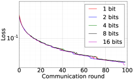
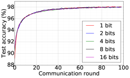
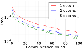
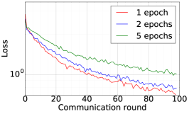
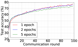
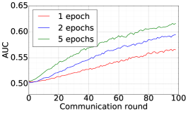
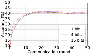
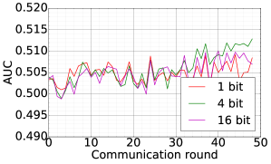
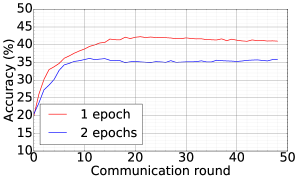
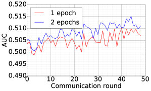
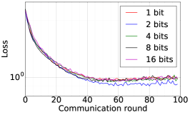
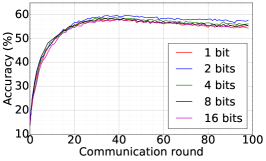
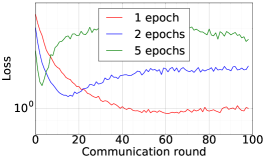
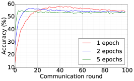
We train two DNNs for MNIST classification using 100 clients: 1) A simple multilayer-perceptron with 2-hidden layers with 200 units each using ReLU activation (199,210 total parameters), which we refer to as 2NN. 2) A CNN with two convolution layers (the first with 32 channels, the second with 64, each followed with max pooling), a fully connected layer with 512 units and ReLU activation, and the final output layer (1,663,370 total parameters). We study two partitioning of the MNIST data over clients, i.e., IID and Non-IID. In IID setting, the data is shuffled, and then partitioned into 20 clients each receiving 3000 examples. In Non-IID, we first sort the data by digit label, divide it into 40 shards of size 1500, and assign each of 20 clients 2 shards. In training, we set the local batch size (batch size of the training data on clients) to be 50, learning rate 0.01, and momentum 0.9. Figures 2 and 3 show the results of training CNN for MNIST classification (Fig. 2: IID and Fig. 3 Non-IID) by DFedAvgM using different communication bits and different local epochs. These results confirm the efficiency of DFedAvgM for training DNNs; in particular, when the clients’ data are IID. For both IID and Non-IID settings, the communication bits do not affect the performance of DFedAvgM; as we see that the training loss, test accuracy, and AUC under the membership inference attack are almost identical. Increasing local training epochs can accelerate training for IID setting at the cost of faster privacy leakage. However, for Non-IID, increasing local training epochs does not help DFedAvgM in either training or privacy protection. Training 2NN by DFedAvgM behaves similarly, see Figs. 4 and 5.
 |
 |
 |
| CR vs. Training loss | CR vs. Test acc | CR vs. AUC |
 |
 |
 |
| CR vs. Training loss | CR vs. Test acc | CR vs. AUC |
 |
 |
 |
| CR vs. Training loss | CR vs. Test acc | CR vs. AUC |
 |
 |
 |
| CR vs. Training loss | CR vs. Test acc | CR vs. AUC |
 |
 |
 |
| CR vs. Training loss | CR vs. Test acc | CR vs. AUC |
 |
 |
 |
| CR vs. Training loss | CR vs. Test acc | CR vs. AUC |
 |
 |
 |
| CR vs. Training loss | CR vs. Test acc | CR vs. AUC |
 |
 |
 |
| CR vs. Training loss | CR vs. Test acc | CR vs. AUC |
Comparison between DFedAvgM, FedAvg, and DSGD.
Now, we compare the DFedAvgM, FedAvg, and DSGD in training 2NNs for MNIST classification. We use the same local batch size 50 for both FedAvg and DSGD, and the learning rates are both set to 0.1444We note that DFedAvg requires smaller learning rates than FedAvg and DSGD for numerical convergence.. For FedAvg, we select all clients to get involved in training and communication in each round. Figure 6 compares three algorithms in terms of test loss and test accuracy for IID MNIST over communication round and communication cost. In terms of communication rounds, DFedAvgM converges as fast as FedAvg, and both are much faster than DSGD. DFedAvgM has a significant advantage over FedAvg and DSGD in communication costs. For Non-IID MNIST, training 2NN by FedAvg can achieve 96.81% test accuracy, but both DFedAvg and DSGD cannot bypass 85%. This disadvantage is because both DSGD and DFedAvgM only communicate with their neighbors, while the neighbors and itself may not contain enough training data to cover all possible classes. One feasible solution to resolve the issues of DFedAvgM for the Non-IID setting is by designing a new graph structure for more efficient global communication.
 |
 |
| CR vs. Test loss | CB vs. Test loss |
 |
 |
| CR vs. Test acc | CB vs. Test acc |
6.2 LSTM for Language Modeling
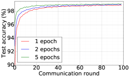
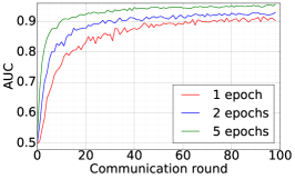
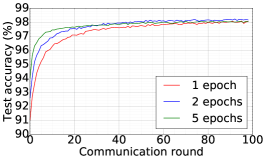
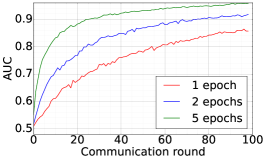
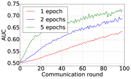
We consider the SHAKESPEARE dataset and we follow the processing as that used in [1], resulting in a dataset distributed over 1146 clients in the Non-IID fashion. On this data, we use DFedAvgM to train a stacked character-level LSTM language model, which predicts the next character after reading each character in a line. The model takes a series of characters as input and embeds each of these into a learned 8-dimensional space. The embedded characters are then processed through 2 LSTM layers, each with 256 nodes. Finally, the output of the second LSTM layer is sent to a softmax output layer with one node per character. The full model has 866,578 parameters, and we trained using an unroll length of 80 characters. We set the local batch size to 10, and we use a learning rate of 1.47, which is the same as [1]. The momentum is selected to be 0.9. Figure 7 plots the communication round vs. test accuracy and AUC under MIA for different quantization and different local epochs. These results show that 1) both the accuracy and MIA increase as training goes; 2) higher communication cost can lead to faster convergence; 3) increase local epochs deteriorate the performance of DFedAvgM.
 |
 |
| CR vs. Test accuracy | CR vs. AUC |
 |
 |
| CR vs. Test accuracy | CR vs. AUC |
6.3 CIFAR10 Classification
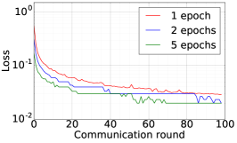
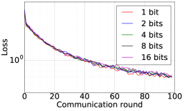
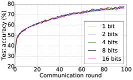
Finally, we use DFedAvgM to train ResNet20 for CIFAR10 classification, which consists of 10 classes of images with three channels. There are 50,000 training and 10,000 testing examples, which we partitioned into 20 clients uniformly, and we only consider the IID setting following [1]. We use the same data augmentation and DNN as that used in [1]. The local batch size is set to 50, the learning rate is set to 0.01, and the momentum is set to 0.9. Figure 8 shows the communication round vs. test accuracy and AUC under MIA for different quantization and different local epochs. If the local epoch is set to 1, different communication bits does not lead to a significant difference in training loss, test accuracy, and AUC under MIA. However, for the fixed communication bits 16, increase the local epochs from 1 to 2 or to 5 will make training not even converge.
 |
 |
 |
| CR vs. Training loss | CR vs. Test acc | CR vs. AUC |
 |
 |
 |
| CR vs. Training loss | CR vs. Test acc | CR vs. AUC |
7 Concluding Remarks
In this paper, we proposed a DFedAvgM and its quantized version. There two major benefits of the DFedAvgM over the existing FedAvg: 1) In FedAvg, communication between the central parameter server and local clients is required in each communication round, and this communication will be very expensive as the number of clients is very large. On the contrary, in DFedAvgM communications are between clients which are significantly less than FedAvg. 2) In FedAvg, the central server collects the updated models from clients, and attack the central server can break the privacy of the whole system. In contrast, conceptually, it is harder to break the privacy in DFedAvgM than FedAvg. Furthermore, we established the theoretical convergence for DFedAvgM and its quantized version under general nonconvex assumptions, and we showed that the worst-case convergence rate of (quantized) DFedAvgM is the same as that of DSGD. In particular, we proved a sublinear convergence rate of (quantized) DFedAvgM when the objective functions satisfy the PŁ condition. We perform extensive numerical experiments to verify the efficacy of DFedAvgM and its quantized version in training ML models and protect membership privacy.
References
- [1] H. B. Mcmahan, E. Moore, D. Ramage, S. Hampson, and B. A. Y. Arcas, “Communication-efficient learning of deep networks from decentralized data,” pp. 1273–1282, 2017.
- [2] H. Robbins and S. Monro, “A stochastic approximation method,” Annals of Mathematical Statistics, vol. 22, no. 3, pp. 400–407, 1951.
- [3] M. Zinkevich, M. Weimer, L. Li, and A. J. Smola, “Parallelized stochastic gradient descent,” in Advances in neural information processing systems, pp. 2595–2603, 2010.
- [4] X. Lian, C. Zhang, H. Zhang, C.-J. Hsieh, W. Zhang, and J. Liu, “Can decentralized algorithms outperform centralized algorithms? a case study for decentralized parallel stochastic gradient descent,” in Advances in Neural Information Processing Systems, pp. 5330–5340, 2017.
- [5] A. Lalitha, S. Shekhar, T. Javidi, and F. Koushanfar, “Fully decentralized federated learning,” in Third workshop on Bayesian Deep Learning (NeurIPS), 2018.
- [6] A. Lalitha, O. C. Kilinc, T. Javidi, and F. Koushanfar, “Peer-to-peer federated learning on graphs,” arXiv preprint arXiv:1901.11173, 2019.
- [7] I. Sutskever, J. Martens, G. Dahl, and G. Hinton, “On the importance of initialization and momentum in deep learning,” in International conference on machine learning, pp. 1139–1147, 2013.
- [8] T.-M. H. Hsu, H. Qi, and M. Brown, “Measuring the effects of non-identical data distribution for federated visual classification,” arXiv preprint arXiv:1909.06335, 2019.
- [9] S. J. Reddi, Z. Charles, M. Zaheer, Z. Garrett, K. Rush, J. Konečný, S. Kumar, and H. B. McMahan, “Adaptive federated optimization,” in International Conference on Learning Representations, 2021.
- [10] T. Chen, G. Giannakis, T. Sun, and W. Yin, “Lag: Lazily aggregated gradient for communication-efficient distributed learning,” in Advances in Neural Information Processing Systems, pp. 5050–5060, 2018.
- [11] J. Sun, T. Chen, G. Giannakis, and Z. Yang, “Communication-efficient distributed learning via lazily aggregated quantized gradients,” in Advances in Neural Information Processing Systems, pp. 3365–3375, 2019.
- [12] T. Li, A. K. Sahu, M. Zaheer, M. Sanjabi, A. Talwalkar, and V. Smithy, “Feddane: A federated newton-type method,” in 2019 53rd Asilomar Conference on Signals, Systems, and Computers, pp. 1227–1231, IEEE, 2019.
- [13] A. Khaled, K. Mishchenko, and P. Richtárik, “First analysis of local gd on heterogeneous data,” arXiv preprint arXiv:1909.04715, 2019.
- [14] X. Li, K. Huang, W. Yang, S. Wang, and Z. Zhang, “On the convergence of fedavg on non-IID data,” in International Conference on Learning Representations, 2020.
- [15] H. B. McMahan et al., “Advances and open problems in federated learning,” Foundations and Trends® in Machine Learning, vol. 14, no. 1, 2021.
- [16] T. Li, A. K. Sahu, A. Talwalkar, and V. Smith, “Federated learning: Challenges, methods, and future directions.,” arXiv: Learning, 2019.
- [17] S. Boyd, A. Ghosh, B. Prabhakar, and D. Shah, “Gossip algorithms: Design, analysis and applications,” in INFOCOM 2005. 24th Annual Joint Conference of the IEEE Computer and Communications Societies. Proceedings IEEE, vol. 3, pp. 1653–1664, IEEE, 2005.
- [18] R. Olfati-Saber, J. A. Fax, and R. M. Murray, “Consensus and cooperation in networked multi-agent systems,” Proceedings of the IEEE, vol. 95, no. 1, pp. 215–233, 2007.
- [19] L. Schenato and G. Gamba, “A distributed consensus protocol for clock synchronization in wireless sensor network,” in 2007 46th ieee conference on decision and control, pp. 2289–2294, IEEE, 2007.
- [20] T. C. Aysal, M. E. Yildiz, A. D. Sarwate, and A. Scaglione, “Broadcast gossip algorithms for consensus,” IEEE Transactions on Signal processing, vol. 57, no. 7, pp. 2748–2761, 2009.
- [21] A. Nedic and A. Ozdaglar, “Distributed subgradient methods for multi-agent optimization,” IEEE Transactions on Automatic Control, vol. 54, no. 1, pp. 48–61, 2009.
- [22] A. I. Chen and A. Ozdaglar, “A fast distributed proximal-gradient method,” in Communication, Control, and Computing (Allerton), 2012 50th Annual Allerton Conference on, pp. 601–608, IEEE, 2012.
- [23] D. Jakovetić, J. Xavier, and J. M. Moura, “Fast distributed gradient methods,” IEEE Transactions on Automatic Control, vol. 59, no. 5, pp. 1131–1146, 2014.
- [24] I. Matei and J. S. Baras, “Performance evaluation of the consensus-based distributed subgradient method under random communication topologies,” IEEE Journal of Selected Topics in Signal Processing, vol. 5, no. 4, pp. 754–771, 2011.
- [25] K. Yuan, Q. Ling, and W. Yin, “On the convergence of decentralized gradient descent,” SIAM Journal on Optimization, vol. 26, no. 3, pp. 1835–1854, 2016.
- [26] J. Zeng and W. Yin, “On nonconvex decentralized gradient descent,” IEEE Transactions on Signal Processing, vol. 66, no. 11, pp. 2834–2848, 2018.
- [27] B. Sirb and X. Ye, “Consensus optimization with delayed and stochastic gradients on decentralized networks,” in Big Data (Big Data), 2016 IEEE International Conference on, pp. 76–85, IEEE, 2016.
- [28] G. Lan, S. Lee, and Y. Zhou, “Communication-efficient algorithms for decentralized and stochastic optimization,” Mathematical Programming, vol. 180, no. 1, pp. 237–284, 2020.
- [29] X. Lian, W. Zhang, C. Zhang, and J. Liu, “Asynchronous decentralized parallel stochastic gradient descent,” in Proceedings of the 35th International Conference on Machine Learning, pp. 3043–3052, 2018.
- [30] T. Sun, P. Yin, D. Li, C. Huang, L. Guan, and H. Jiang, “Non-ergodic convergence analysis of heavy-ball algorithms,” in Proceedings of the AAAI Conference on Artificial Intelligence, vol. 33, pp. 5033–5040, 2019.
- [31] R. Xin and U. A. Khan, “Distributed heavy-ball: A generalization and acceleration of first-order methods with gradient tracking,” IEEE Transactions on Automatic Control, 2019.
- [32] A. Reisizadeh, A. Mokhtari, H. Hassani, and R. Pedarsani, “Quantized decentralized consensus optimization,” in 2018 IEEE Conference on Decision and Control (CDC), pp. 5838–5843, IEEE, 2018.
- [33] Q. Yang, Y. Liu, Y. Cheng, Y. Kang, T. Chen, and H. Yu, Federated learning. Morgan & Claypool Publishers, 2019.
- [34] H. Xing, O. Simeone, and S. Bi, “Decentralized federated learning via SGD over wireless D2D networks,” in 2020 IEEE 21st International Workshop on Signal Processing Advances in Wireless Communications (SPAWC), pp. 1–5, IEEE, 2020.
- [35] T. Li, A. K. Sahu, M. Zaheer, M. Sanjabi, A. Talwalkar, and V. Smith, “Federated optimization in heterogeneous networks,” Proceedings of the 1 st Adaptive & Multitask Learning Workshop, Long Beach, California, 2019.
- [36] S. Ghadimi and G. Lan, “Stochastic first-and zeroth-order methods for nonconvex stochastic programming,” SIAM Journal on Optimization, vol. 23, no. 4, pp. 2341–2368, 2013.
- [37] S. Boyd, P. Diaconis, and L. Xiao, “Fastest mixing markov chain on a graph,” SIAM review, vol. 46, no. 4, pp. 667–689, 2004.
- [38] B. T. Polyak, “Some methods of speeding up the convergence of iteration methods,” Ussr Computational Mathematics and Mathematical Physics, vol. 4, no. 5, pp. 1–17, 1964.
- [39] M. Li, D. G. Andersen, A. J. Smola, and K. Yu, “Communication efficient distributed machine learning with the parameter server,” in Advances in Neural Information Processing Systems, pp. 19–27, 2014.
- [40] D. Alistarh, D. Grubic, J. Li, R. Tomioka, and M. Vojnovic, “QSGD: Communication-efficient SGD via gradient quantization and encoding,” in Advances in Neural Information Processing Systems, pp. 1709–1720, 2017.
- [41] S. Magnússon, H. Shokri-Ghadikolaei, and N. Li, “On maintaining linear convergence of distributed learning and optimization under limited communication,” IEEE Transactions on Signal Processing, vol. 68, pp. 6101–6116, 2020.
- [42] H. Karimi, J. Nutini, and M. Schmidt, “Linear convergence of gradient and proximal-gradient methods under the polyak-łojasiewicz condition,” in Joint European Conference on Machine Learning and Knowledge Discovery in Databases, pp. 795–811, Springer, 2016.
- [43] S. J. Reddi, A. Hefny, S. Sra, B. Poczos, and A. Smola, “Stochastic variance reduction for nonconvex optimization,” in International conference on machine learning, pp. 314–323, 2016.
- [44] D. J. Foster, A. Sekhari, and K. Sridharan, “Uniform convergence of gradients for non-convex learning and optimization,” in Advances in Neural Information Processing Systems, pp. 8745–8756, 2018.
- [45] B. T. Polyak, “Gradient methods for minimizing functionals,” Zhurnal Vychislitel’noi Matematiki i Matematicheskoi Fiziki, vol. 3, no. 4, pp. 643–653, 1963.
- [46] S. Lojasiewicz, “A topological property of real analytic subsets,” Coll. du CNRS, Les équations aux dérivées partielles, vol. 117, pp. 87–89, 1963.
- [47] S. Shalev-Shwartz, Y. Singer, N. Srebro, and A. Cotter, “Pegasos: Primal estimated sub-gradient solver for svm,” Mathematical programming, vol. 127, no. 1, pp. 3–30, 2011.
- [48] A. Nemirovski, A. Juditsky, G. Lan, and A. Shapiro, “Robust stochastic approximation approach to stochastic programming,” SIAM Journal on optimization, vol. 19, no. 4, pp. 1574–1609, 2009.
- [49] A. Salem, Y. Zhang, M. Humbert, P. Berrang, M. Fritz, and M. Backes, “Ml-leaks: Model and data independent membership inference attacks and defenses on machine learning models,” In Annual Network and Distributed System Security Symposium (NDSS 2019), 2019.