Decentralized Motion Planning with Collision Avoidance for a Team of UAVs under High Level Goals
Abstract
This paper addresses the motion planning problem for a team of aerial agents under high level goals. We propose a hybrid control strategy that guarantees the accomplishment of each agent’s local goal specification, which is given as a temporal logic formula, while guaranteeing inter-agent collision avoidance. In particular, by defining -D spheres that bound the agents’ volume, we extend previous work on decentralized navigation functions and propose control laws that navigate the agents among predefined regions of interest of the workspace while avoiding collision with each other. This allows us to abstract the motion of the agents as finite transition systems and, by employing standard formal verification techniques, to derive a high-level control algorithm that satisfies the agents’ specifications. Simulation and experimental results with quadrotors verify the validity of the proposed method.
I Introduction
Multi-agent systems have received a significant amount of attention over the last decades. The complexity of many tasks, such as assembling parts and heavy/large object transportation or manipulation, necessitates the employment of a group of robots, rather than a single one, since it offers greater versatility, redundancy and fault tolerance.
In the case of aerial vehicles, tasks involving area coverage/inspection or rescue missions point out the importance of using multi-agent setups. The standard problem of formation control for a team of aerial vehicles is addressed in [1, 2, 3, 4, 5, 6], whereas [7, 8, 9, 10, 11] consider leader-follower formation approaches, where the latter also treats the problem of collision avoidance with static obstacles in the environment; [12], [13] and [14] employ dynamic programming, Model Predictive Control and reachable set algorithms, respectively, for inter-agent collision avoidance. In [15] the cooperative evader pursuit problem is treated.
Ultimately, however, we would like the aerial robots to execute more complex high-level tasks, involving combinations of safety ("never enter a dangerous regions"), surveillance ("keep visiting regions and infinitely often") or sequencing ("collect data in region and upload it in region ") properties. Temporal logic languages offer a means to express the aforementioned specifications, since they can describe complex planning objectives in a more efficient way than the well-studied navigation algorithms. Recently, the incorporation of temporal logic-based planning to the robotics and automation field has gained a considerable amount of attention, both in single- and multi-agent setups [16, 17, 18, 19, 20, 21, 22, 23, 24, 25, 26, 27]. Regarding aerial vehicles, [28] addresses the vehicle routing problem using MTL specifications and [29] approaches the LTL motion planning using MILP optimization techniques, both in a centralized manner. Markov Decision Processes are used for the LTL planning in [30]. The aforementioned works, however, consider discrete agent models and do not take into account their continuous dynamics.
Another important feature in multi-agent planning and control is the need for decentralization and minimization of inter-agent communication; centralized approaches, where a central system computes the overall team plan or cases where the agents communicate online with each other, can cause computationally expensive procedures, even for small robot teams. In the case of temporal logics, the use of product transition systems incorporating the states of all agents (as e.g., in [25, 17, 30]) can render the solution to the motion planning problem practically infeasible.
Moreover, the majority of works in the related literature of temporal logic-based motion planning considers point-agents (as, e.g. in [19, 24, 23]) and does not take into account potential collisions between them. The latter is a crucial safety property in real-time scenarios, where actual vehicles are used in the motion planning framework.
In this work, we propose a novel decentralized control protocol for the motion planning of a team of aerial vehicles under LTL specifications with simultaneous inter-agent collision avoidance. In particular, we extend previous work on decentralized navigation functions [31] to abstract the motion of each agent as a finite transition system. Then, we employ standard formal-verification techniques to derive plans that satisfy each agent’s LTL specification. The proposed control protocol is decentralized in the sense that each agent has limited sensing information and derives and executes its desired path without communicating with the other agents or knowing their respective goals/specifications. Simulation and experimental results with quadrotors verify the effectiveness of the proposed framework. To the best of the authors’ knowledge, this is the first approach that integrates temporal logic-based motion planning with decentralized navigation functions in an experimental framework with UAVs.
The rest of the paper is organized as follows: Section II introduces notation and preliminary background. Section III describes the problem formulation and the overall system’s model. The control strategy is presented in Section IV. Sections V and VI verify our approach through numerical simulations and experiments, respectively, and Section VII concludes the paper.
II Notation and Preliminaries
Vectors and matrices are denoted with bold lowercase and uppercase letters, respectively, whereas scalars are denoted with non-bold letters. The set of positive integers is denoted as and the real -coordinate space, with , as ; is the set of real -vectors will all elements nonnegative; denotes the ball of radius and center ; Moreover, given a set , the notation denotes the interior of , is the set of all subsets of and, given a finite sequence of elements in , with , we denote by the infinite sequence created by repeating . Finally, is the -dimensional Euclidean distance, with .
II-A Specification in LTL
We focus on the task specification given as a Linear Temporal Logic (LTL) formula. The basic ingredients of a LTL formula are a set of atomic propositions and several boolean and temporal operators. LTL formulas are formed accoding to the following grammar [32]: , where and (next), (until). Definitions of other useful operators like (always), (eventually) and (implication) are omitted and can be found in [32].
The semantics of LTL are defined over infinite words over . Intuitively, an atomic proposition is satisfied on a word if it holds at its first position , i.e. . Formula holds true if is satisfied on the word suffix that begins in the next position , whereas states that has to be true until becomes true. Finally, and holds on eventually and always, respectively. For a full formal definition of the LTL semantics, the reader is kindly referred to [32].
II-B Navigation Functions
Navigation functions, first introduced in [33], are real valued maps realized through cost functions, whose negated gradient field is attractive towards the goal configuration and repulsive with respect to obstacles. A navigation function can be formally defined as follows:
Definition 1
Let be a compact connected analytic manifold with boundary. A map is a navigation function if: (1) It is analytic on , (2) it has only one minimum , (3) its Hessian at all critical points (zero gradient field) is full rank and (4), .
Following [33], given a spherical workspace centered at with radius , an initial position ,a goal position and spherical obstacles with center and radius , respectively for , a choice for a navigation function in is , with:
| (1) |
where is a design parameter, , with , is the attractive potential towards the goal and , with , is the repulsive potential from the workspace boundary and the obstacles, where and ; reaches its minimal value only at and its maximal value at the boundaries of the workspace and the obstacles. It has been shown that by following the negated gradient , it is guaranteed for sufficiently large that and , for almost all initial positions .
III System and Problem Formulation
Consider aerial agents operating in a static workspace that is bounded by a large sphere in -D space , where and are the center and radius of . Within there exist smaller spheres around points of interest, which are described by , where are the central point and radius, respectively, of . We denote the set of all as . For the workspace partition to be valid, we consider that the regions of interest are sufficiently distant from each other and from the workspace boundary, i.e., and with . Moreover, we introduce a set of atomic propositions for each agent that indicates certain properties of interest of agent in and are expressed as boolean variables. The properties satisfied at each region are provided by the labeling function , which assigns to each region the subset of the atomic propositions that are true in that region.
III-A System model
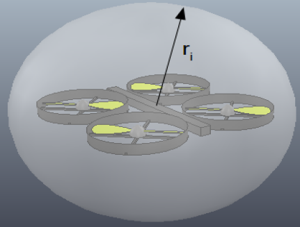
Each agent occupies a bounding sphere: , where is the center and the radius of the sphere (Fig. 1). We also consider that , i.e., the regions of interest are larger than the aerial vehicles. The motion of each agent is controlled via its centroid through the single integrator dynamics:
| (2) |
Moreover, we consider that agent has a limited sensing range of . Therefore, by defining the neighboring set , agent knows at each time instant the position of all as well as its own position . The workspace is perfectly known, i.e., are known to all agents, for all .
With the above ingredients, we provide the following definitions:
Definition 2
An agent is in a region at a configuration , denoted as , if and only if .
Definition 3
Assume that for some . Then there exists a transition for agent from region to region , denoted as , if and only if there exists a finite and a bounded control trajectory such that (i) , (ii) , and (iii) with with and .
Loosely speaking, an agent can transit between two regions of interest and , if there exists a bounded control trajectory in (2) that takes agent from to while avoiding entering all other regions and colliding with the other agents.
III-B Specification
Our goal is to control the multi-agent system subject to (2) so that each agent’s behavior obeys a given specification over its atomic propositions .
Given a trajectory of agent , its corresponding behavior is given by the infinite sequence , with and .
Definition 4
The behavior satisfies an LTL formula if and only if .
III-C Problem Formulation
The control objectives are given for each agent separately as LTL formulas over . An LTL formula is satisfied if there exists a behavior of agent that satisfies . Formally, the problem treated in this paper is the following:
Problem 1
Given a set of aerial vehicles subject to the dynamics (2) and LTL formulas over the respective atomic propositions , achieve behaviors that (i) yield satisfaction of and (ii) guarantee inter-agent collision avoidance.
IV Main Results
IV-A Continuous Control Design
The first ingredient of our solution is the development of a decentralized feedback control law that establishes a transition relation according to Def. 3. First, we provide an overview of the concept of Decentralized Navigation Functions, introduced in [31], that we will use in the subsequent analysis.
IV-A1 Decentralized Navigation Functions (DNFs)
Consider agents described by the position variables , bounding spheres , sensing radius and dynamics as in (2). Each agent’s goal is to reach a desired position without colliding with the other agents. To this end, we employ the following class of decentralized navigation functions: , with , where and . The function is defined as and it represents the attraction of agent towards its goal position, with being the desired set. The term is associated with the collision avoidance property of agent with the rest of the team and is based on the inter-agent distance function [31]: with
that represents the distance between agents and . Roughly speaking, expresses all possible collisions between agent and the others and is the set we want to avoid. The term is introduced in [31] and is used in this work in order to avoid inter-agent collisions in the case where with , i.e., when two or more agents have the same goal positions and they approach them simultaneously. Analytic expressions for and can be found in [31]. With the aforementioned tools, the control law for agent is , which, as shown in [31], drives all agents to their goal positions and guarantees inter-agent collision-avoidance.
IV-A2 Continuous Control Law
By employing the aforementioned ideas regarding DNFs and given that for some , we propose a decentralized control law for the transition , as defined in Def. 3.
Initially, we define the set of "undesired" regions as and the corresponding free space . As the goal configuration we consider the centroid of and we construct the function with . For the collision avoidance between the agents, we employ the function as defined in [31].
Moreover, we also need some extra terms that guarantee that agent will avoid the rest of the regions as well as the workspace boundary. To this end, we construct the function with , where the function is a measure of the distance of agent from the workspace boundary and the function is a measure of the distance of agent from the undesired regions .
With the above ingredients, we construct the following navigation function :
| (3) |
for agent , with and the following vector field:
| (4) |
for all , with and as defined in [31].
The navigation field (4) guarantees that agent will not enter the undesired regions or collide with the other agents and . The latter property of asymptotic convergence along with the assumption that , implies that there exists a finite time instant such that and more specifically that , which is the desired behavior. The time instant can be chosen from the set .
Note, however, that once agent leaves region , there is no guarantee that it will not enter that region again (note that includes ). Therefore, we define the set and the corresponding free space , and we construct the function :
| (5) |
where , with corresponding vector field:
| (6) |
which guarantees that region will be also avoided. Therefore, we develop a switching control protocol that employs (4) until agent is out of region and then switches to (6) until . Consider the following switching function:
| (7) |
where is the standard saturation function (, if , if ), and the time instant that represents the moment that agent is out of region , i.e., , where . Note that , since with . Then, we propose the following switching control protocol :
| (8) |
where and , where is a design parameter indicating the time period of the switching process, with . Invoking the continuity of , we obtain and hence the control protocol (8) guarantees, for sufficiently small , that agent will navigate from to in finite time without entering any other regions or colliding with other agents and therefore establishes a transition . The proof of correctness of (3) and (5) follows closely the one in [31] and is therefore omitted.
IV-B High-Level Plan Generation
The next step of our solution is the high-level plan, which can be generated using standard techniques inspired by automata-based formal verification methodologies. In Section IV-A, we proposed a continuous control law that allows the agents to transit between any in the given workspace , without colliding with each other. Thanks to this and to our definition of LTL semantics over the sequence of atomic propositions, we can abstract the motion capabilities of each agent as a finite transition system as follows [32]:
Definition 5
The motion of each agent in is modeled by the following Transition System (TS):
| (9) |
where is the set of states represented by the regions of interest that the agent can be at, according to Def. 2, is the set of initial states that agent can start from, is the transition relation established in Section IV-A, abbreviated as , and are the atomic propositions and labeling function respectively, as defined in Section III.
After the definition of , we translate each given LTL formula into a Büchi automaton and we form the product . The accepting runs of satisfy and are directly projected to a sequence of waypoints to be visited, providing therefore a desired path for agent . Although the semantics of LTL is defined over infinite sequences of atomic propositions, it can be proven that there always exists a high-level plan that takes a form of a finite state sequence followed by an infinite repetition of another finite state sequence. For more details on the followed technique, we kindly refer the reader to the related literature, e.g., [32].
Following the aforementioned methodology, we obtain a high-level plan for each agent as sequences of regions and atomic propositions and with and .
The execution of produces a trajectory that corresponds to the behavior , with and , . Therefore, since , the behavior yields satisfaction of the formula . Moreover, the property of inter-agent collision avoidance is inherent in the transition relations of and guaranteed by the navigation control algorithm of Section IV-A. The previous discussion is summarized in the following theorem:
Theorem 1
The individual executions of , that satisfy the respective , produce agent behaviors that (i) yield the satisfaction of all and (ii) guarantee inter-agent collision avoidance, providing, therefore, a solution to Problem 1.
Remark 1
The proposed control algorithm is decentralized in the sense that each agent derives and executes its own plan without communicating with the rest of the team. The only information that each agent has is the position of its neighboring agents that lie in its limited sensing radius.
V Simulation Results
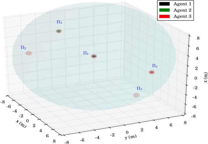
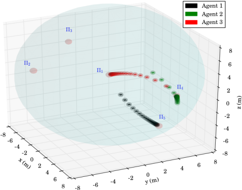
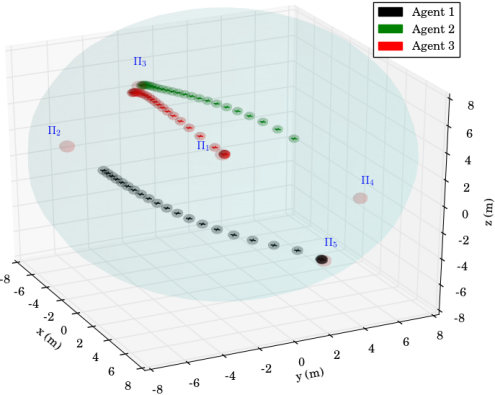
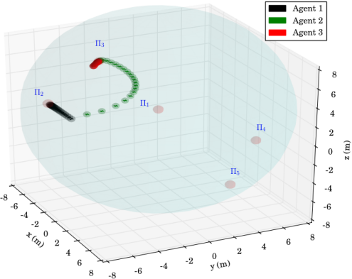
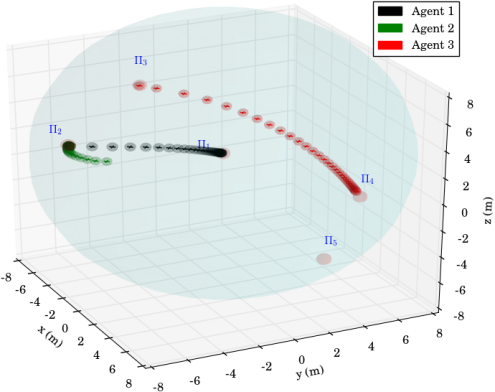
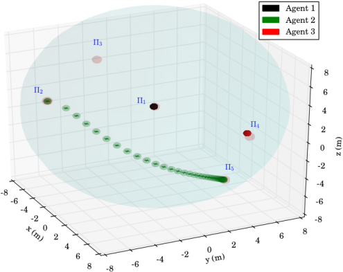
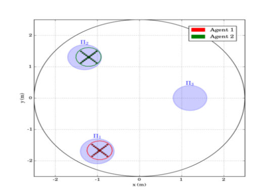
To demonstrate the efficiency of the proposed algorithm, we consider aerial vehicles , with m, m, , operating in a workspace with m and m. Moreover, we consider spherical regions of interest with m, and m, m, m, m and m. The initial configurations of the agents are taken as and therefore, and . An illustration of the described workspace is depicted in Fig. 2.
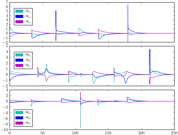
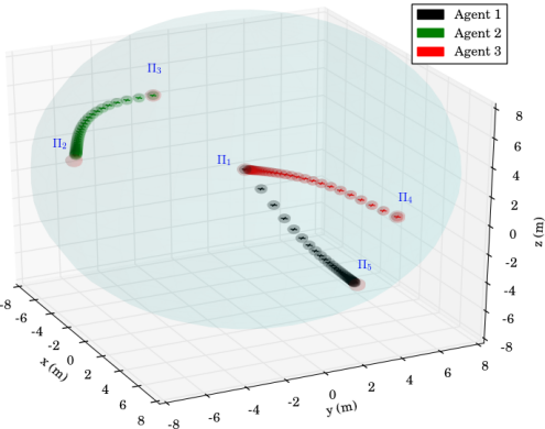
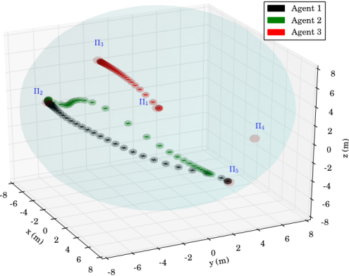
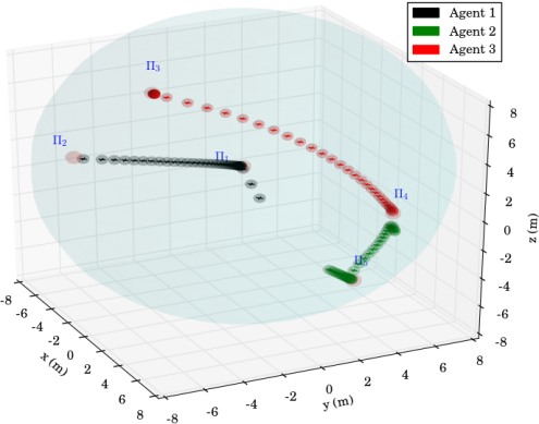
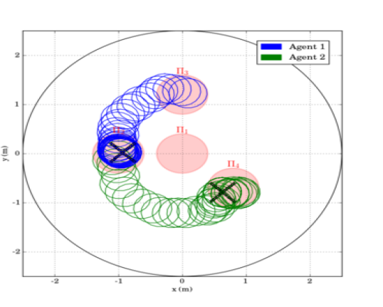
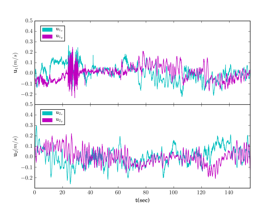
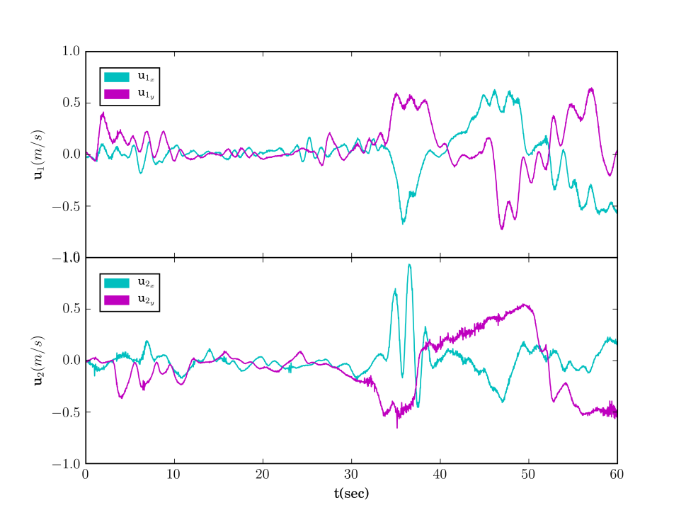
We consider that agent is assigned with inspection tasks and has the atomic propositions with and , where we have considered that region is an undesired ("obstacle") region for this agent. More specifically, the task for agent is the continuous inspection of the workspace while avoiding region . The corresponding LTL specification is . Agents and are interested in moving around resources scattered in the workspace and have propositions with and . We assume that is shared between the two agents whereas and have to be accessed only by agent and and only by agent . The corresponding specifications are and , where we have also included a specific order for the access of the resources. Next, we employ the off-the-shelf tool LTL2BA [34] to create the Büchi automata and by following the procedure described in Section IV-B, we derive the paths , whose execution satisfies . Regarding the continuous control protocol, we chose in (4), (6) and the switching duration in (8) was calculated online as , where we assume that the large distance between the regions (see Fig. 2) implies that and thus, . The simulation results are depicted in Fig. 3 and 5. In particular, Fig. 5 illustrates the execution of the paths and by agents and respectively, where the superscript here denotes that the corresponding paths are executed twice. Fig. 3 depicts the resulting control inputs . The figures demonstrate the successful execution of the agents’ paths and therefore, satisfaction of the respective formulas with inter-agent collision avoidance.
VI Experimental Results
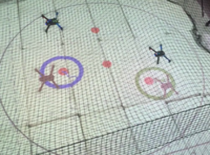
The validity and efficiency of the proposed solution was also verified through real-time experiments. The experimental setup involved two remotely controlled IRIS+ quadrotors from D Robotics, which we consider to have sensing range m, upper control input bound m/s, , and bounding spheres with radius m, . We considered two -dimensional scenarios in a workspace , i.e. and m.
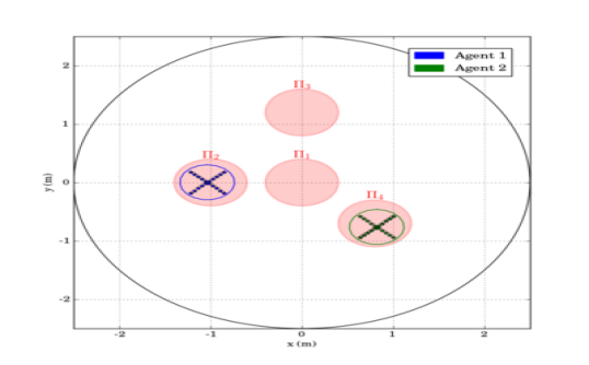
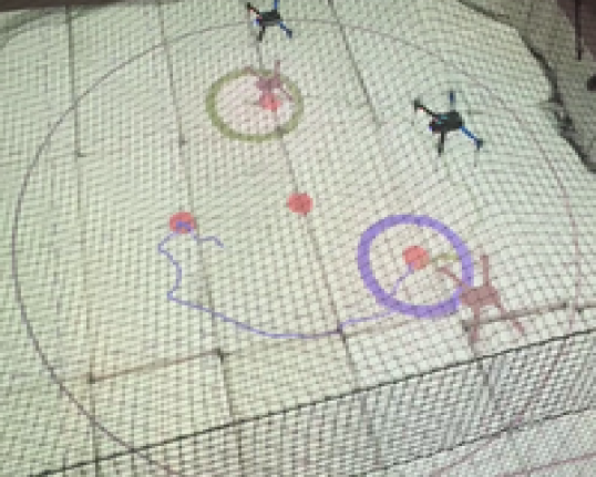
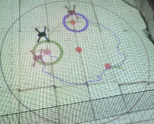
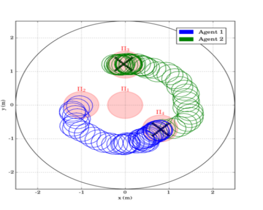
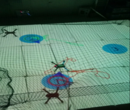
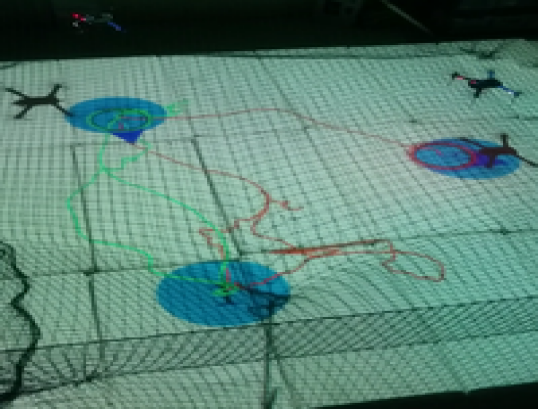
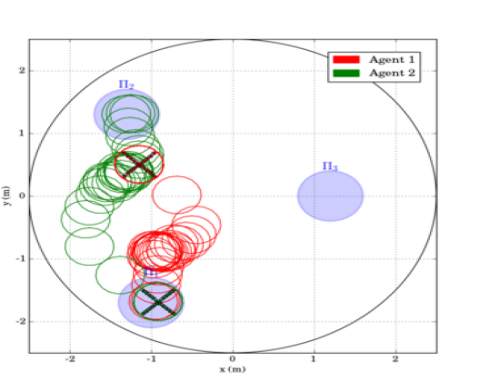
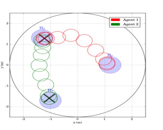
The first scenario included regions of interest in , with and m, m, m and m. The initial positions of the agents were taken such that and (see Fig. 4). We also defined the atomic propositions with . In this scenario, we were interested in area inspection while avoiding the "obstacle" region, and thus, we defined the individual specifications with the following LTL formulas: . By following the procedure described in Section IV-B, we obtained the paths . Fig. 6 depicts the execution of the paths and by agents and , respectively, and Fig. 7 shows the corresponding input signals, which do not exceed the control bounds m/s. It can be deduced by the figures that the agents successfully satisfy their individual formulas, without colliding with each other.
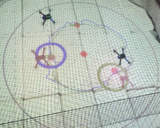
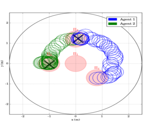
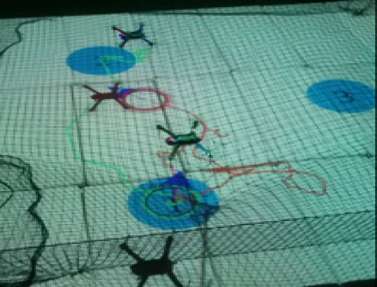
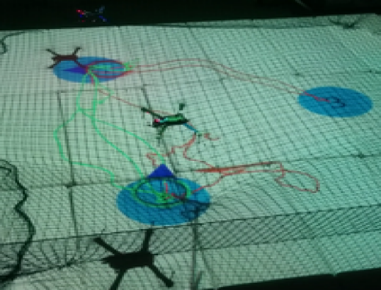
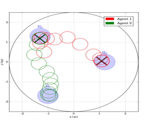
The second experimental scenario included regions of interest in , with and m, m and m. The initial positions of the agents were taken such that and (see Fig. 8). We also defined the atomic propositions , corresponding to a base and several resources in the workspace, with . We considered that the agents had to transfer the resources to the "base" in ; both agents were responsible for but only agent should access . The specifications were translated to the formulas and the derived paths were and . The execution of the paths and by agents 1 and 2, respectively, are depicted in Fig. 10, and the corresponding control inputs are shown in Fig. 9. The figures demonstrate the successful execution and satisfaction of the paths and formulas, respectively, and the compliance with the control input bounds.
Regarding the continuous control protocol in the aforementioned experiments, we chose in (4), (6) and the switching duration in (8) as .
Remark 2
Note that, although the limited available workspace in the experiments did not satisfy all the conditions regarding the distance between regions and the workspace boundary, as introduced in Section III, the two experimental scenarios were successfully conducted.
The simulations and experiments were conducted in Python environment using an Intel Core i7 2.4 GHz personal computer with 4 GB of RAM, and are clearly demonstrated in the video found in https://youtu.be/dO77ZYEFHlE, a compressed version of which has been submitted with this paper.
VII Conclusion and Future Work
In this work, we proposed a control strategy for the motion planning of a team of aerial vehicles under LTL specifications. By using decentralized navigation functions that guarantee inter-agent collision avoidance, we abstracted each agent’s motion as a finite transition system between regions of interest. Each agent then derived the plan that satisfies its given LTL formula through formal-verification techniques. Simulation studies and experimental results verified the efficiency of the proposed algorithm. Future efforts will be devoted towards considering more complex, second order dynamics, partially known environments and experiments with more agents.
References
- [1] S. Liu, C. Wang, G. Liang, H. Chen, and X. Wu, “Formation control strategy for a group of quadrotors,” in IEEE International Conference on Information and Automation (ICIA), 2015.
- [2] B. Yu, X. Dong, Z. Shi, and Y. Zhong, “Formation control for quadrotor swarm systems: Algorithms and experiments,” in Chinese Control Conference (CCC), 2013.
- [3] N. Koeksal, B. Fidan, and K. Bueyuekkabasakal, “Real-time implementation of decentralized adaptive formation control on multi-quadrotor systems,” in European Control Conference (ECC), 2015.
- [4] Z. Hou and I. Fantoni, “Composite nonlinear feedback-based bounded formation control of multi-quadrotor systems,” in European Control Conference (ECC), 2016.
- [5] R. L. Pereira and K. H. Kienitz, “Tight formation flight control based on h-infinity approach,” in Mediterranean Conference on Control and Automation (MED), 2016.
- [6] X. Dong, B. Yu, Z. Shi, and Y. Zhong, “Time-varying formation control for unmanned aerial vehicles: Theories and applications,” IEEE Transactions on Control Systems Technology, 2015.
- [7] D. A. Mercado, R. Castro, and R. Lozano, “Quadrotors flight formation control using a leader-follower approach,” in European Control Conference (ECC), 2013.
- [8] V. Roldao, R. Cunha, D. Cabecinhas, C. Silvestre, and P. Oliveira, “A novel leader-following strategy applied to formations of quadrotors,” in European Control Conference (ECC), 2013.
- [9] S. Ulrich, “Nonlinear passivity-based adaptive control of spacecraft formation flying,” in American Control Conference (ACC), 2016.
- [10] N. D. Hao, B. Mohamed, H. Rafaralahy, and M. Zasadzinski, “Formation of leader-follower quadrotors in cluttered environment,” in American Control Conference (ACC), 2016.
- [11] K. A. Ghamry and Y. Zhang, “Formation control of multiple quadrotors based on leader-follower method,” in International Conference on Unmanned Aircraft Systems (ICUAS), 2015.
- [12] Z. N. Sunberg, M. J. Kochenderfer, and M. Pavone, “Optimized and trusted collision avoidance for unmanned aerial vehicles using approximate dynamic programming,” in IEEE International Conference on Robotics and Automation (ICRA), 2016.
- [13] A. Eskandarpour and V. J. Majd, “Cooperative formation control of quadrotors with obstacle avoidance and self collisions based on a hierarchical mpc approach,” in RSI/ISM International Conference on Robotics and Mechatronics (ICRoM), 2014.
- [14] Y. Zhou and J. S. Baras, “Reachable set approach to collision avoidance for uavs,” in IEEE Conference on Decision and Control (CDC), 2015.
- [15] A. Pierson, A. Ataei, I. C. Paschalidis, and M. Schwager, “Cooperative multi-quadrotor pursuit of an evader in an environment with no-fly zones,” in IEEE International Conference on Robotics and Automation (ICRA), 2016.
- [16] M. M. Quottrup, T. Bak, and R. I. Zamanabadi, “Multi-robot planning : a timed automata approach,” in IEEE International Conference on Robotics and Automation (ICRA), 2004.
- [17] S. G. Loizou and K. J. Kyriakopoulos, “Automated planning of motion tasks for multi-robot systems,” in IEEE Conference on Decision and Control, 2005.
- [18] I. Filippidis, D. V. Dimarogonas, and K. J. Kyriakopoulos, “Decentralized multi-agent control from local ltl specifications,” in IEEE Conference on Decision and Control (CDC), 2012.
- [19] M. Guo and D. V. Dimarogonas, “Multi-agent plan reconfiguration under local ltl specifications,” Internatinal Journal on Robotics Research, 2015.
- [20] V. Nenchev and C. Belta, “Receding horizon robot control in partially unknown environments with temporal logic constraints,” in IEEE European Control Conference (ECC), 2016.
- [21] S. Feyzabadi and S. Carpin, “Multi-objective planning with multiple high level task specifications,” in IEEE International Conference on Robotics and Automation (ICRA), 2016.
- [22] M. Guo, J. Tumova, and D. V. Dimarogonas, “Hybrid control of multi-agent systems under local temporal tasks and relative-distance constraints,” in IEEE Conference on Decision and Control (CDC), 2015.
- [23] G. E. Fainekos, A. Girard, H. Kress-Gazit, and G. J. Pappas, “Temporal logic motion planning for dynamic robots,” Automatica, 2009.
- [24] M. Kloetzer and C. Belta, “Ltl planning for groups of robots,” in IEEE International Conference on Networking, Sensing and Control, 2006.
- [25] A. Ulusoy, S. L. Smith, X. C. Ding, C. Belta, and D. Rus, “Optimality and robustness in multi-robot path planning with temporal logic constraints,” The International Journal of Robotics Research, 2013.
- [26] Z. Zhang and R. V. Cowlagi, “Motion-planning with global temporal logic specifications for multiple nonholonomic robotic vehicles,” in American Control Conference (ACC), 2016.
- [27] D. Aksaray, C.-I. Vasile, and C. Belta, “Dynamic routing of energy-aware vehicles with temporal logic constraints,” IEEE International Conference on Robotics and Automation (ICRA), 2016.
- [28] S. Karaman and E. Frazzoli, “Vehicle routing problem with metric temporal logic specifications,” in IEEE Conference on Decision and Control (CDC), 2008.
- [29] ——, “Complex mission optimization for multiple-uavs using linear temporal logic,” in American Control Conference (ACC), 2008.
- [30] J. Xiaoting and N. Yifeng, “Robust strategy planning for uav with ltl specifications,” in Chinese Control Conference (CCC), 2016.
- [31] D. V. Dimarogonas and K. J. Kyriakopoulos, “Decentralized navigation functions for multiple robotic agents with limited sensing capabilities,” Journal of Intelligent and Robotic Systems, 2007.
- [32] C. Baier, J.-P. Katoen et al., Principles of model checking. MIT press Cambridge, 2008.
- [33] D. E. Koditschek and E. Rimon, “Robot navigation functions on manifolds with boundary,” Advances in Applied Mathematics, 1990.
- [34] P. Gastin and D. Oddoux, LTL2BA tool, 2012. [Online]. Available: http://www.lsv.ens-cachan.fr/ gastin/ltl2ba/.