Decoherence and degradation of squeezed states in quantum filter cavities
Abstract
Squeezed states of light have been successfully employed in interferometric gravitational-wave detectors to reduce quantum noise, thus becoming one of the most promising options for extending the astrophysical reach of the generation of detectors currently under construction worldwide. In these advanced instruments, quantum noise will limit sensitivity over the entire detection band. Therefore, to obtain the greatest benefit from squeezing, the injected squeezed state must be filtered using a long-storage-time optical resonator, or “filter cavity”, so as to realise a frequency dependent rotation of the squeezed quadrature. Whilst the ultimate performance of a filter cavity is determined by its storage time, several practical decoherence and degradation mechanisms limit the experimentally achievable quantum noise reduction. In this paper we develop an analytical model to explore these mechanisms in detail. As an example, we apply our results to the filter cavity design currently under consideration for the Advanced LIGO interferometers.
pacs:
04.80.Nn, 42.50.Dv, 04.30.-w, 42.50.LcI Introduction
Squeezed states of light are used in a variety of experiments in optical communication, biological sensing and precision measurement Takeda et al. (2013); Taylor et al. (2013); Yonezawa et al. (2012). To gravitational-wave detectors, the finest position-meters ever built, squeezed states of light today represent one of the most mature technologies for further expanding the detectable volume of the universe The LIGO Scientific Collaboration (2011, 2013).
The advanced detectors currently under construction, such as Advanced LIGO Harry and the LIGO Scientific Collaboration (2010), will be limited by quantum noise over their entire detection band, from 10 Hz to 10 kHz. To fully exploit the potential of squeezing, squeezed states must therefore be manipulated so as to impress a frequency dependent rotation upon the squeezing ellipse. Such rotation can be realised by reflecting the squeezed states from a detuned, over-coupled, optical resonator, called a quantum filter cavity.
The performance of ideal filter cavities, fundamentally limited by their storage times, is well-understood Kimble et al. (2001); Harms et al. (2003) and a proof-of-principle experimental demonstration has been performed Chelkowski et al. (2005). However, the impact of several decoherence and degradation mechanisms which critically determine the achievable performance of astrophysically relevant filter cavities has not yet been investigated.
In this paper we present an analytical model, based on the two-photon formalism Caves and Schumaker (1985); Schumaker and Caves (1985); Corbitt et al. (2005), which evaluates the reduction in observable squeezing caused by optical losses and by spatial mode mismatch between the injected squeezed light, the filter cavity and the interferometer. Further, we also explore the influence of squeezed quadrature fluctuations Dwyer (2013), or “phase noise”, generated both inside and outside the filter cavity. As a concrete example, we study the effects of these noise sources on a 16 m long filter cavity with a 60 Hz linewidth, parameters considered for Advanced LIGO Evans et al. (2013).
II Analytical model
The frequency dependent squeezing system modelled in this work is shown in Figure 1. The squeezed beam is injected into the interferometer after reflection from the filter cavity. In this model we assume that the quantum noise enhancement is measured via a generic homodyne readout system, by beating the interferometer output field against a local oscillator (LO) field. The main sources of squeezing decoherence (optical loss and mode-mismatch) and degradation (phase noise due to local-oscillator phase-lock errors and cavity length fluctuations) are indicated.
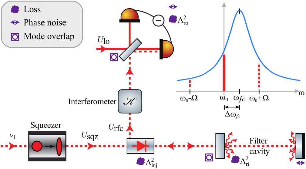
Using the mathematical formalism described in Evans et al. (2013) and further developed in appendix A, our analysis calculates the achievable quantum noise reduction by propagating three classes of vacuum field through the optical system: which passes through the squeezer and becomes the squeezed field; which accounts for all vacuum fluctuations that are coupled into the beam due to optical losses before the interferometer; and which accounts for vacuum fluctuations introduced due to losses after the interferometer. In this formalism vacuum fields are proportional to the identity matrix, , and their interaction with an optical element or system may be described by multiplication with a transmission matrix , i.e. .
In sections II.1, II.2 and II.3 we develop transfer matrices for the propagation of through the squeezer and injection optics, its modification by the filter cavity and the influence it experiences due imperfect mode-matching. Section II.4 constructs a transfer matrix describing the optomechanical coupling of the interferometer and shows that it can be written as a product of rotation and squeezing operators. We then, in section II.5, incorporate the uncontrolled vacuum noise coupled into the squeezed field due to loss and show how one can compute the quantum noise at the readout of the interferometer using the matrices developed in the previous sections. The final piece of our analytical model, performance degradation due to phase noise, is detailed in section II.6.
II.1 Squeezed field injection
The squeezer is represented by the operator , given by
| (1) |
which describes squeezing by at angle and anti-squeezing by at . Conventionally, squeezing magnitudes are expressed in decibels (dB), with .
In general, all optical losses outside of the filter cavity are frequency independent or the frequency dependence is so small that it can be neglected. Examples of optical losses are residual transmissions of steering mirrors, scattering, absorption and imperfections in polarisation optics. The last of these is likely to dominate the frequency-independent losses incurred in the passage of the squeezed field to the readout, therefore these losses are represented in Figure 1 as occurring at the optical isolator.
Since there are no non-linear elements in our system between the squeezer and the interferometer (i.e. nothing which mixes upper and lower audio sidebands) we can combine all of the input losses together into a single frequency-independent “injection loss”, , which represents the total power loss outside of the filter cavity and before the readout (this work does not consider any losses within the interferometer itself).
Amalgamating the losses with the action of the squeezer, we arrive at the two-photon transfer matrix which takes to the filter cavity111Our model treats all injection losses as occurring before the filter cavity. This approach is valid as the action of the filter cavity on coherent vacuum states is null.,
| (2) |
where the attenuation due to is described by the transfer coefficient .
II.2 Filter cavity
Reflection from a filter cavity is a linear process which can easily be described in the one-photon, and therefore two-photon, formalisms, as in equation (A9) of Evans et al. (2013). However, the approach therein does not permit one to explore the consequences of filter cavity imperfections analytically, with resulting loss of physical insight. Here we revisit this equation and, by making appropriate approximations, construct a closed-form expression for the action of a filter cavity in the two-photon formalism.
For a given signal sideband frequency , the complex reflectivity, , of a filter cavity, using the same notation as Evans et al. (2013), is given by
| (3) |
where is the amplitude reflectivity of the input mirror and is the cavity’s round-trip amplitude reflectivity. For a cavity of length and resonant frequency , the round-trip phase is defined as
| (4) |
where is the cavity detuning with respect to the carrier frequency and is the speed of light.
For a high-finesse cavity near to resonance, we can make the approximations
| (5) | ||||
| (6) |
where accounts for the power lost during one round-trip in the cavity (not including input mirror transmission).
Under these approximations, and neglecting terms of order 1 or greater in , and , (3) can be rewritten as 222Note that the defined here is similar to that in equation (94) of Kimble et al. (2001) and that for an optimally coupled cavity.
| (7) | ||||
| (8) | ||||
| (9) |
and the cavity half-width-half-maximum-power linewidth is defined as
| (10) |
As noted by previous authors Khalili (2010), for a given cavity half-width , the filter cavity performance is determined entirely by the loss per unit length .
To investigate the effect the filter cavity has on a squeezed field we must convert its response, (7), into the two-photon picture. This is done with the one-photon to two-photon conversion matrix (see Evans et al. (2013) and section A.3),
| (11) |
yielding the transfer matrix
| (12) |
where .
To cast this expression in a more instructive form, we require several sum and difference quantities based on . In terms of and , the complex phase and magnitude of are given by
| (13) | ||||
| (14) |
Whence we define
| (15) |
where the subscripts and are used to denote the sum and difference of the phases and magnitudes.
The transfer matrix of the filter cavity can then be expressed in a form which clearly shows the effect of intra-cavity loss,
| (16) |
where is the 22 identity matrix.
The first term in this expression, marked “lossless”, consists of a rotation operation and an overall phase which are identical to the rotation and phase provided by a lossless filter cavity Kimble et al. (2001).
The second,“lossy”, term goes to unity for a lossless filter cavity ( and ). However, in the presence of losses, this term mixes the quadratures of the squeezed state, corrupting “squeezing” with “anti-squeezing”. We emphasise that this effect is not decoherence, as we have not yet introduced the vacuum fluctuations which enter as a consequence of the filter cavity losses, but rather a coherent dephasing of the squeezed quadratures which cannot be undone by rotation of the state. This dephasing is a direct result of different reflection magnitudes experienced by the upper and lower audio sidebands (i.e. ). The ramifications of this effect on the measured noise are presented in section II.5.
Additionally, by combining (13) and (II.2), we are now able to write an explicit expression for the squeezed quadrature rotation, , produced by the filter cavity,
| (17) |
which holds for typical filter cavity parameters, . In particular, for a lossless filter cavity (),
| (18) |
consistent with the expression for which can be deduced from (88) of Kimble et al. (2001) (note that the referenced equation is missing factor of 2, as reported in Harms et al. (2003)).
II.3 Mode-matching
A quantum filter cavity modifies the phase of the squeezed state which is coupled into its resonant mode. In a laboratory context, free-space optics are used to perform this coupling, maximising the spatial overlap between the cavity mode and the incident beam. This process is known as “mode-matching” and the result is inevitably imperfect. In the case of quantum filter cavities, imperfect mode-matching results in both a source of loss and in a path by which the squeezed state can bypass the filter cavity. In this section we develop a model describing how imperfect filter cavity mode-matching affects a squeezed state. Furthermore, we also include the effects of loss arising from mode-mismatch between the squeezed field and the beam, known as the “local oscillator” (LO), used to detect it.
The previously stated filter cavity reflectivity applies only to a field perfectly mode-matched to the cavity fundamental mode. In order to incorporate mode-mismatch, we express the LO and the beam from the squeezed light source in an orthonormal basis of spatial modes (e.g. Hermite-Gauss or Laguerre-Gauss modes) such that
| (19) | ||||
| (20) |
where and are complex coefficients. We further choose this basis such that is the filter cavity fundamental mode. For the beam from the squeezed light source is perfectly matched to the filter cavity mode. Similarly, indicates that the local oscillator beam has perfectly spatial overlap with the filter cavity mode.
Since the filter cavity is held near the resonance of the fundamental mode, we assume that all other modes ( with ) are far from resonance, with and . Thus, the squeezed beam after reflection from the filter cavity is given by
| (21) |
The fundamental mode’s amplitude and phase are modified by the filter cavity, whereas those of the other modes remain unchanged since these modes are not resonant and the filter cavity acts like a simple mirror.
The spatial overlap integral of the reflected field and the local oscillator is
| (22) |
where Note that represents the overlap between the mismatched part of the beam from the squeezed light source and the mismatched LO. The squeezed field which follows this path essentially bypasses the filter cavity, and thereby experiences no frequency dependent rotation. It may, however, acquire a frequency independent rotation with respect to the field which couples into the filter cavity, as can be seen from the two-photon mode-mismatch matrix
| (23) |
The addition of this coupling path results in a frequency dependent rotation error with respect to the rotation expected from a perfectly mode matched filter cavity. For modest amounts of mode-mismatch (less than ), this error can be corrected by a small change in the filter cavity detuning.
The magnitude of the mode-mismatch is constrained by such that
| (24) |
while the phase is in general unconstrained. The overlap is maximised when is real and positive and minimised when it is real and negative.
Experimentally, the quantities which one can easily measure are the squeezed field/filter cavity power mode-coupling, , and the squeezed field/local oscillator power mode-coupling, , say. From these values one can determine , the overlap between the LO and filter cavity modes, in the following way,
| (25) |
where captures the ambiguity in the phase. The parameters of interest for noise propagation are then easily determined,
| (26) | ||||
| (27) |
Note that the second equality in (25) is not universally true. The magnitude of the second term (the expression multiplying the exponential) can be smaller than that given, depending on the unknown character of the mode-mismatches. However this choice, an upper bound, allows one to explore the full range of values necessary to constrain the mode-mismatch-induced noise.
II.4 Interferometer
The non-linear action of radiation pressure in an interferometer affects any vacuum field incident upon it. In our analysis, we include an idealised lossless interferometer to illustrate this phenomenon. Operated on resonance, such an interferometer may be described by the transfer matrix
| (28) |
as reported in Buonanno and Chen (2001). Here, characterises the coupling of amplitude fluctuations introduced at the interferometer’s dark port to phase fluctuations exiting the same port and takes the form
| (29) |
where is the interferometer signal-bandwidth and is a characteristic frequency, dependent on the particular interferometer configuration, which approximates the frequency at which the interferometer quantum noise equals the Standard Quantum Limit (i.e. where radiation pressure noise intersects shot noise Kimble et al. (2001)).
For a conventional interferometer without a signal recycling mirror, like the power-recycled Michelson interferometer described in Kimble et al. (2001),
| (30) | ||||
| (31) |
where is the laser power stored inside the interferometer arm cavities, is the frequency of the carrier field, is the arm cavity length, is the mass of each test mass mirror, is the power transmissivity of the arm cavity input mirrors and approximations are valid provided arm cavity finesse is high.
| Parameter | Symbol | Value |
| Frequency of the carrier field | ||
| Arm cavity length | ||
| Signal recycling cavity length | ||
| Arm cavity half-width | ||
| Arm cavity input mirror power | ||
| transmissivity | ||
| Signal recycling mirror power | ||
| transmissivity | ||
| Intra-cavity power | ||
| Mass of each of the test mass mirror |
For a dual-recycled interferometer, operating with a tuned signal-recycling cavity of length , it can be shown that, for ,
| (32) | ||||
| (33) |
where and are the amplitude transmissivity and reflectivity of the signal recycling mirror. Given the Advanced LIGO parameters reported in Table 1,
| (34) | |||||
| (35) |
confirming that the effect of signal recycling in Advanced LIGO is to increase the interferometer’s bandwidth whilst reducing the frequency at which its quantum noise reaches the SQL. For such an interferometer, in which , may be approximated by in the region of interest (where is order unity or larger).
While (28) is very simple, greater appreciation of the action of the interferometer can be gained by noting that can be recast in terms of the previously defined squeeze and rotation operators as
| (36) |
with
The role of the filter cavity is to rotate the input squeezed quadrature as a function of frequency such that it is always aligned with the signal quadrature at the output of the interferometer, even in the presence of rotation by and the effective rotation caused by squeezing at angle . The required filter cavity rotation is given by
| (37) |
II.5 Linear noise transfer
We now combine the intermediate results of previous sections to compute the quantum noise observed in the interferometer readout. Three vacuum fields make contributions to this noise: which passes through the squeezer, which enters before the interferometer but does not pass through the squeezer and which enters after the interferometer. We formulate transfer matrices for each of these fields in turn before providing, in (43), a final expression for the measured noise.
Converting the result of (22) into a two-photon transfer matrix and including losses in the injection and readout paths, via and respectively (see (2) and (42)), we arrive at the full expression describing the transfer of vacuum field through the squeezer, filter cavity and interferometer to the detection point,
| (38) |
We now consider the vacuum field , which accounts for all fluctuations coupled into the beam due to injection losses, losses inside the filter cavity itself and imperfect mode-matching. The audio-sideband transmission coefficient from the squeezer to the interferometer is
| (39) |
In the two-photon picture, the average of the upper and lower sideband losses gives the source term for the vacuum fluctuations, so that
| (40) | ||||
| (41) |
Finally, frequency independent losses between the interferometer and the readout introduce a second source of attenuation of the squeezed state and accompanying vacuum fluctuations , a process described by the following transfer matrix and transmission coefficient
| (42) |
These losses cannot be added to the injection losses mentioned above since they are separated by the non-linear effects of the interferometer. Explicitly, losses before and after the interferometer are not equivalent.
The single-sided power spectrum of the quantum noise at the interferometer readout is then given by
| (43) |
where the local oscillator field , with amplitude , determines the readout quadrature. All mathematical operations are as defined in Evans et al. (2013) and is defined such that is the noise in the quadrature containing the interferometer signal.
We now investigate (43) more closely, providing analytical expressions for the contribution of each term. To improve readability, we normalise all noise powers with respect to shot noise (see appendix A.2). This action is denoted through the use of an additional circumflex, i.e. rather than .
II.5.1 Noise due to vacuum fluctuations passing through the squeezer,
As the only term with dependence on filter cavity performance, examination of allows one to determine the optimal filter cavity parameters.
A comprehensive expression for may be developed starting from (38). However, for clarity, and to assist in gaining physical understanding, we restrict our discussion to an optimally matched filter cavity, and neglect injection and readout losses, to obtain a simple description in terms of the optomechanical coupling constant , the cavity rotation angle and reflectivities and . In this case,
| (44) |
Equation (44) elucidates both the effect of a filter cavity and the role of filter cavity losses. We first remark that in the absence of both squeezed light () and a filter cavity (equivalent to , ) the interferometer output noise is simply
| (45) |
With the addition of frequency-independent squeezed light (, ), the total output noise becomes
| (46) |
In the frequency region in which the noise is reduced by the presence of squeezed light but for the noise is degraded by the “anti-squeezing” component . Had we chosen these roles would have been reversed.
The presence of a filter cavity () allows one to minimise the impact of “anti-squeezing” on the measured noise. For a lossless filter cavity (, ) the “anti-squeezing” can be completely nulled by selecting filter cavity parameters such that , giving the minimal quantum noise
| (47) |
With the addition of filter cavity losses () the total noise becomes
| (48) |
and there is no value of for which the influence of “anti-squeezing” can be completely nulled (due to the coherent dephasing effect discussed above in II.2). It is important to highlight that precluding “optimal” rotation is not the only downside of a lossy filter cavity. Intra-cavity losses also introduce additional vacuum fluctuations, , which do not pass through the squeezer, leading to increased noise in the interferometer readout via the transfer matrix. Considering an optimally mode-matched filter cavity, this effect is most noticeable in (41), which becomes simply (see also section II.5.2 below).
For an interferometer in which , like a power-recycled Michelson interferometer (or a detuned signal-recycled Michelson interferometer), a single filter cavity is not capable of realising the desired rotation of the squeezed quadrature, as extensively described in section V and appendix C of Kimble et al. (2001). Conversely, for a broadband interferometer like Advanced LIGO, in which and the approximation holds, it can be shown, from (17) and (37), that the output noise is minimised by a single filter cavity with the following parameters
| (49) | ||||
| (50) |
from which the requirements for a lossless filter cavity () can be derived,
| (51) | ||||
| (52) |
In practice, for fixed cavity length and losses, the value of is tuned to obtain the required filter cavity bandwidth. However, changing affects both and , making (50) inconvenient to solve. Nevertheless, equating the right-hand side of (50) with the expression for derived from (8), one obtains a version of which is independent of ,
| (53) |
and can be used to find and . Then, from (10),
| (54) |
We note that as filter cavity losses increase, the ideal filter cavity bandwidth also increases, whilst the optimal cavity detuning is reduced. As a consequence, the desired value of is approximately constant for .
II.5.2 Noise due to vacuum fluctuations which do not pass through the squeezer,
II.5.3 Noise due to vacuum fluctuations in the readout,
The noise due to vacuum fluctuations entering at the interferometer readout follows trivially from (42),
| (57) |
II.6 Phase noise
In addition to optical losses and mode-mismatch, a further cause of squeezing degradation is phase noise, also referred to as “squeezed quadrature fluctuations” Dwyer (2013). In this section we develop a means of quantifying the impact of this important degradation mechanism.
Assuming some parameter in or has small, Gaussian-distributed fluctuations with variance , the average readout noise is given by
| (58) | ||||
| (59) |
Extending this approach to multiple incoherent noise parameters yields
| (60) | ||||
| (61) |
where the parameters not explicitly listed as arguments to , including , are assumed to take on their mean values.
While (61) is sufficient to evaluate for any collection of phase noise sources, we choose to follow the same approach adopted in the treatment of optical losses, considering two classes of squeezed quadrature fluctuations: extra-cavity fluctuations which are frequency independent and intra-cavity fluctuations which are frequency dependent.
Examples of frequency-independent phase noise sources include length fluctuations in the squeezed field injection path and instabilities in the relative phase of the local oscillator or the radio-frequency sidebands which co-propagate with the squeezed field. Such frequency-independent noise may be represented by variations, , in the homodyne readout angle .
Frequency-dependent phase noise is caused by variability in the filter cavity detuning (see (4)). This detuning noise results from filter cavity length noise , driven by seismic excitation of the cavity mirrors or sensor noise associated with the filter cavity length control loop, according to
| (62) |
Detuning noise gives rise to frequency-dependent phase noise through the properties of the filter cavity resonance. For example, the dependence of on is weak for , i.e. for frequencies far from resonance, and stronger for , i.e. for frequencies close to resonance.
General analytic expressions for as a function of and are neither concise nor especially edifying. Therefore, in the following section, we apply (61) numerically to illustrate the impact of phase noise in a typical advanced gravitational-wave detector.
III A 16 m filter cavity for Advanced LIGO
We now apply the analytical model expounded above to the particular case of a 16 m filter cavity. Such a system has recently been considered for application to Advanced LIGO Evans et al. (2013) and therefore we use the specifications of this interferometer in our study (see Table 1).
The remaining parameters, show in Table 2, represent what we believe is technically feasible using currently available technology. For example, the filter cavity length noise estimate assumes that the cavity mirrors will be held in single-stage suspension systems located on seismically isolated HAM-ISI tables Evans (2012) and that the filter cavity length control loop will have 150 Hz unity gain frequency, and whilst a 2% mode-mismatch between the squeezed field and the filter cavity is extremely small, newly developed actuators Kasprzack et al. (2013); Liu et al. (2013) allow us to be optimistic. We chose to inject of squeezing into our system as this value results in of high-frequency squeezing at the interferometer readout (a goal for second-generation interferometers The LIGO Scientific Collaboration (2013)) and, conservatively, to consider a filter cavity with 16 ppm round-trip loss, even if recent investigations have shown that lower losses are achievable Isogai et al. (2013).
| Parameter | Symbol | Value |
| Filter cavity length | ||
| Filter cavity half-bandwidth | ||
| Filter cavity detuning | ||
| Filter cavity input | ||
| mirror transmissivity | ||
| Filter cavity losses | ||
| Injection losses | ||
| Readout losses | ||
| Mode-mismatch losses | ||
| (squeezer-filter cavity) | ||
| Mode-mismatch losses | ||
| (squeezer-local oscillator) | ||
| Frequency independent phase noise (RMS) | ||
| Filter cavity length noise (RMS) | ||
| Injected squeezing |
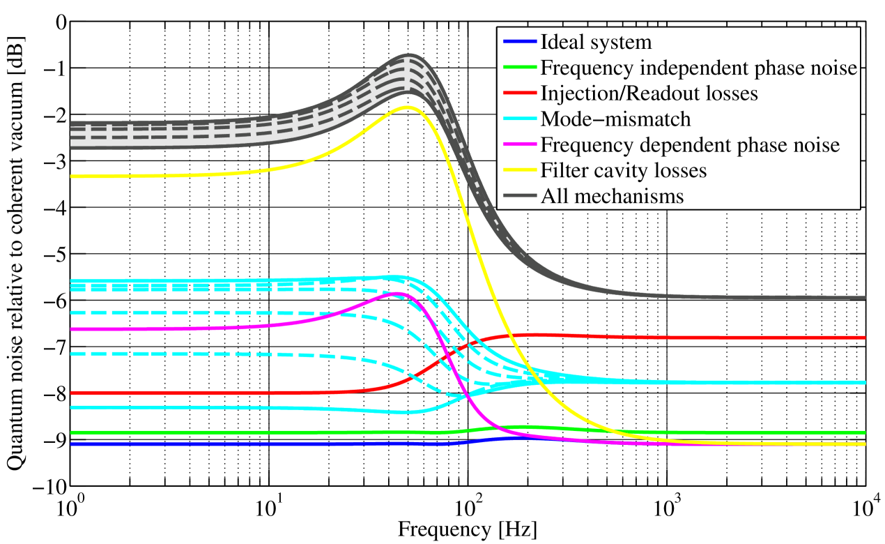
The results of our investigation are shown in Figure 2. One observes that intra-cavity losses are the dominant source of decoherence below . However, we note that, with small changes in parameter choice, the impact of the other coupling mechanisms could also become important. For instance, filter cavity length fluctuations approaching RMS would greatly compromise low frequency performance.
At higher frequencies, injection, readout and mode-mismatch losses are the most influential effects. With total losses of 15%, measuring of squeezing demands that more than 9 dB be present at the injection point.
Even under the idealised condition of negligible filter cavity losses (1ppm/m), achieving a broadband improvement greater than places extremely stringent requirements on the mode-matching throughout the system and on the filter cavity length noise.
IV Conclusions
Quantum filter cavities were proposed several years ago as means of maximising the benefit available from squeezing in advanced interferometric gravitational-wave detectors Kimble et al. (2001). However, the technical noise sources which practically limit filter cavity performance have, until now, been neglected. In this paper we have presented an analytical model capable of quantifying the impact of several such noise sources, including optical loss, mode-mismatch and frequency dependent phase noise. We find that real-world decoherence and degradation can be significant and therefore must be taken into account when evaluating the overall performance of a filter cavity. Applying our model to the specific case of Advanced LIGO Evans et al. (2013), we conclude that a 16 m filter cavity, built with currently available technology, offers considerable performance gains and remains a viable and worthwhile near-term upgrade to the generation of gravitational-wave detectors presently under construction.
Appendix A Formalism
In this appendix we place the calculations presented above in the context of the one-photon and two-photon formalisms extensively discussed in literature (see e.g. Corbitt et al. (2005); Buonanno and Chen (2001)). We commence by connecting the one-photon expression for the time-varying part of the electromagnetic field to power fluctuations on a photo-detector. We then transform the derived expression into the two-photon basis to explicitly show how vacuum fluctuations generate measurable noise. This calculation is subsequently generalised to the case of multiple vacuum fields arriving at a photo-detector after having propagated through an optical system, revealing the origin of (43). Finally, we discuss how quantum noise may be calculated for systems best described in the one-photon picture, in the process deriving the one-photon to two-photon conversion matrix (11).
A.1 One-photon and two-photon in context
The one-photon and two-photon formalisms provide two alternative ways of expressing fields. In the one-photon formalism, as described by (2.6) of Buonanno and Chen (2001), the time varying part of the electromagnetic field is written in terms of its audio-sideband components around the carrier frequency ,
| (63) |
where is the “effective area”, “h.c.” means Hermitian conjugate and are the normalised amplitudes of the upper and lower sidebands at frequencies in dimensions of (see Caves and Schumaker (1985) for greater detail).
By introducing defined as
| (64) |
and noting that Buonanno and Chen (2001) uses , can be rewritten as
| (65) |
where we have introduced the time-dependent amplitude
| (66) |
In our application these fluctuations arrive to the photo-detector together with a strong, constant local oscillator field such that
| (67) |
The power transported by the beam can then be written as
| (68) |
where denotes intensity and the overbar indicates the average over one or more cycles of the electromagnetic wave. Note that the effective area has cancelled and does not have a meaningful effect on the measurable power. Since , we can approximate the power fluctuation as
| (69) |
Switching to the frequency domain, we take the Fourier transform of to find
| (70) |
where, in the final step, we have used (66).
The two-photon formalism defines quadrature fields as linear combinations of the one-photon fields Buonanno and Chen (2001)
| (71) |
such that
| (72) |
By substituting (72) into (70), we obtain the frequency-domain expression for in the two-photon formalism
| (73) |
Expressing the local oscillator’s amplitude and phase explicitly, , becomes
| (74) |
A.2 Calculation of quantum noise
Equation (74) provides a simple method of calculating the power fluctuations on a photo-detector given any time-varying electromagnetic field beating against a local oscillator.
As a specific and relevant example, quantum noise (due to the zero-point energy of the electromagnetic field) drives vacuum fluctuations, and , which are incoherent and of unit amplitude at all frequencies. The resulting noise power generated being
| (75) | ||||
| (76) |
where and have initially been listed explicitly to highlight the incoherent nature of the noise associated with each of the two quadratures. Note that this expression is consistent with the familiar equation for the amplitude spectral density of shot noise, since the average power level is equal to .
The tools of linear algebra can now be exploited to simplify these expressions, allowing one to rewrite the noise as
| (77) |
where the local oscillator is as defined in section II.5 (given the LO phase convention ),
| (78) |
and , simply proportional to the identity matrix, embodies the two independent vacuum noise sources
| (79) |
In general, to calculate the quantum noise in an optical system, the vacuum field entering an open port is propagated to the readout photodetector through the transfer matrix of the system,
| (80) |
as described in Evans et al. (2013). The vacuum fluctuations then beat against the local oscillator field present on the photodetector to give the power spectrum of quantum noise
| (81) |
If multiple paths lead to the same photodetector, the total noise may be calculated as the sum of the contributions due to each vacuum source,
| (82) |
Finally, dividing by the shot noise level gives the normalised noise power used throughout this paper
| (83) |
A.3 One-photon transfer
Some optical systems, like filter cavities, are better described by the one-photon formalism, as this makes their transfer matrices diagonal. As in the two-photon formalism, the quantum noise is the result of the incoherent sum of the noise generated by two vacuum fields. Although, in this case, the fields of concern are and (rather than and ). Beginning from (70), the resulting noise is
| (84) |
where, as before, and have been included explicitly before being set to unity.
However, rather than develop an equivalent set of linear algebra expressions for computing total noise output in the one-photon formalism, we instead use (71) and (72) to define a one-photon to two-photon conversion matrix
| (85) |
The one-photon transfer matrix of any optical system which does not mix upper and lower audio sidebands (i.e. any linear system) can then be expressed in the two-photon formalism as
| (86) |
where are the transfer coefficients for the upper and lower audio sidebands.
Acknowledgements.
The authors gratefully acknowledge the support of the National Science Foundation and the LIGO Laboratory, operating under cooperative Agreement No. PHY-0757058. This paper has been assigned LIGO Document No. LIGO-P1400018.References
- Takeda et al. (2013) S. Takeda, T. Mizuta, M. Fuwa, P. van Loock, and A. Furusawa, Nature 500, 315 (2013).
- Taylor et al. (2013) M. A. Taylor, J. Janousek, V. Daria, J. Knittel, B. Hage, H.-A. Bachor, and W. P. Bowen, Nature Photonics 7, 229 (2013), arXiv:1206.6928 [quant-ph] .
- Yonezawa et al. (2012) H. Yonezawa, D. Nakane, T. A. Wheatley, K. Iwasawa, S. Takeda, H. Arao, K. Ohki, K. Tsumura, D. W. Berry, T. C. Ralph, H. M. Wiseman, E. H. Huntington, and A. Furusawa, Science 337, 1514 (2012), http://www.sciencemag.org/content/337/6101/1514.full.pdf .
- The LIGO Scientific Collaboration (2011) The LIGO Scientific Collaboration, Nature Physics 7, 962 (2011).
- The LIGO Scientific Collaboration (2013) The LIGO Scientific Collaboration, Nature Photonics 7, 613 (2013).
- Harry and the LIGO Scientific Collaboration (2010) G. M. Harry and the LIGO Scientific Collaboration, Classical and Quantum Gravity 27, 084006 (2010).
- Kimble et al. (2001) H. J. Kimble, Y. Levin, A. B. Matsko, K. S. Thorne, and S. P. Vyatchanin, Phys. Rev. D 65, 022002 (2001).
- Harms et al. (2003) J. Harms, Y. Chen, S. Chelkowski, A. Franzen, H. Vahlbruch, K. Danzmann, and R. Schnabel, Phys. Rev. D 68, 042001 (2003).
- Chelkowski et al. (2005) S. Chelkowski, H. Vahlbruch, B. Hage, A. Franzen, N. Lastzka, K. Danzmann, and R. Schnabel, Phys. Rev. A 71, 013806 (2005), arXiv:0706.4479 [quant-ph] .
- Caves and Schumaker (1985) C. M. Caves and B. L. Schumaker, Phys. Rev. A 31, 3068 (1985).
- Schumaker and Caves (1985) B. L. Schumaker and C. M. Caves, Phys. Rev. A 31, 3093 (1985).
- Corbitt et al. (2005) T. Corbitt, Y. Chen, and N. Mavalvala, Phys. Rev. A 72, 013818 (2005), quant-ph/0502088 .
- Dwyer (2013) S. Dwyer, Quantum noise reduction using squeezed states in LIGO, Ph.D. thesis, Massachusetts Institute of Technology (2013).
- Evans et al. (2013) M. Evans, L. Barsotti, P. Kwee, J. Harms, and H. Miao, Phys. Rev. D 88, 022002 (2013), arXiv:1305.1599 [physics.optics] .
- Note (1) Our model treats all injection losses as occurring before the filter cavity. This approach is valid as the action of the filter cavity on coherent vacuum states is null.
- Note (2) Note that the defined here is similar to that in equation 94 of Kimble et al. (2001), and that for an optimally coupled cavity.
- Khalili (2010) F. Y. Khalili, Phys. Rev. D 81, 122002 (2010), arXiv:1003.2859 [physics.ins-det] .
- Buonanno and Chen (2001) A. Buonanno and Y. Chen, Phys. Rev. D 64, 042006 (2001), gr-qc/0102012 .
- Evans (2012) M. Evans, Seismic Noise Spectra for SEI and SUS, Tech. Rep. T1200155 (LIGO Scientific Collaboration, 2012).
- Kasprzack et al. (2013) M. Kasprzack, B. Canuel, F. Cavalier, R. Day, E. Genin, J. Marque, D. Sentenac, and G. Vajente, Appl. Opt. 52, 2909 (2013).
- Liu et al. (2013) Z. Liu, P. Fulda, M. A. Arain, L. Williams, G. Mueller, D. B. Tanner, and D. H. Reitze, Appl. Opt. 52, 6452 (2013).
- Isogai et al. (2013) T. Isogai, J. Miller, P. Kwee, L. Barsotti, and M. Evans, Opt. Express 21, 30114 (2013).