Deep Bayesian Filter for Bayes-Faithful Data Assimilation
Abstract
State estimation for nonlinear state space models (SSMs) is a challenging task. Existing assimilation methodologies predominantly assume Gaussian posteriors on physical space, where true posteriors become inevitably non-Gaussian. We propose Deep Bayesian Filtering (DBF) for data assimilation on nonlinear SSMs. DBF constructs new latent variables in addition to the original physical variables and assimilates observations . By (i) constraining the state transition on the new latent space to be linear and (ii) learning a Gaussian inverse observation operator , posteriors remain Gaussian. Notably, the structured design of test distributions enables an analytical formula for the recursive computation, eliminating the accumulation of Monte Carlo sampling errors across time steps. DBF trains the Gaussian inverse observation operators and other latent SSM parameters (e.g., dynamics matrix) by maximizing the evidence lower bound. Experiments demonstrate that DBF outperforms model-based approaches and latent assimilation methods in tasks where the true posterior distribution on physical space is significantly non-Gaussian.
1 Introduction
Data assimilation (DA) is a crucial technique across various scientific domains. Its primary objective is to estimate the trajectory and current state of a system by integrating an imperfect model with partially informative observations. Specifically, given a series of observations time steps , the goal is to infer the posterior distribution of the system’s physical variables : . DA has been widely applied in fields such as weather forecasting (Hunt et al., 2007; Lorenc, 2003; Andrychowicz et al., 2023), ocean research analysis (Ohishi et al., 2024), sea surface temperature prediction (Larsen et al., 2007), seismic wave analysis (Alfonzo & Oliver, 2020), multi-sensor fusion localization (Bach & Ghil, 2023), and visual object tracking (Awal et al., 2023).
A key challenge in DA arises from the non-Gaussian nature of the posterior distributions , which results from the inherent nonlinearity in both the system dynamics and observation models. Despite this, many operational DA systems, such as those used in weather forecasting, rely on methods like the ensemble Kalman Filter (EnKF) (Evensen, 1994; Bishop et al., 2001) for sequential state filtering (i.e., ) and the four-dimensional variational method (4D-Var) for retrospective state analysis (i.e., ). These approaches assume Gaussianity in their test distributions or , a simplification driven by computational constraints. While exact methods such as bootstrap Particle Filters (PF) or sequential Monte Carlo (SMC) (Chopin & Papaspiliopoulos, 2020; Daum & Huang, 2007; Hu & van Leeuwen, 2021) could compute the true posterior, their performance degrades significantly when the number of particles is insufficient (Beskos et al., 2014). This issue is exacerbated in high-dimensional systems, making SMC approaches impractical for many physical problems.
To address these limitations, we propose a novel variational inference approach called Deep Bayesian Filtering (DBF) for posterior estimation. Our strategy consists of two main components: (i) constraining the test distribution to remain Gaussian to ensure computational tractability, and, in cases where the original dynamics are nonlinear, (ii) leveraging a nonlinear mapping to enhance the expressive capability of the test distribution. The DBF methodology diverges into two paths depending on the nature of the system dynamics, whether linear Gaussian or nonlinear:
Linear dynamics
When the system’s dynamics are linear, DBF assumes Gaussianity in the original space, similar to traditional methods. However, DBF introduces the concept of the inverse observation operator (IOO; see also Frerix et al. 2021) to construct Gaussian test distributions . The IOO, along with any unknown system parameters, are trained to minimize the Kullback-Leibler divergence between the test distribution and the true posterior . The IOO and the system parameters are trained without teacher signals .
Nonlinear dynamics
In the more common case of nonlinear dynamics, DBF operates in a latent space, assuming Gaussianity in the latent variables . The original physical variables are recovered through a nonlinear mapping function , implemented via neural networks (NNs). This nonlinear mapping allows for a more flexible representation of the test distribution . The IOO and other parameters are trained in a supervised manner (i.e., is used during training).
For state space models (SSMs) with nonlinear dynamics, DBF functions as a variational autoencoder (VAE) that adheres to the Markov property. Posterior distributions of the latent variables are expressed in a Bayesian framework. This approach is closely related to dynamical VAEs (DVAEs, Girin et al. 2021 for a review), which use VAEs to model time-series data. However, DBF distinguishes itself by its posterior design. Unlike DVAEs, where Monte Carlo sampling is required for inference (see Sec. 2.6.1), DBF allows for the analytical computation of the prediction step, recursively computing posteriors through closed-form expressions.
When applied to problems with nonlinear or unknown dynamics, DBF can be interpreted as learning the Koopman operator (Koopman, 1931) using NNs. The discovery of such latent spaces and operators through machine learning has been extensively studied (Takeishi et al., 2017; Lusch et al., 2018; Azencot et al., 2020) and will be experimentally validated through the handling of nonlinear filtering tasks involving chaotic dynamics.
Key contributions of the proposed DBF methodology include:
-
•
DBF is the first VAE-based model for time-series data that maintains a posterior structure faithful to the Markov property in SSMs.
-
•
For systems with linear dynamics, DBF extends the Kalman Filter (KF) to handle nonlinear observations through learnable NNs. The training process enables the model to infer unknown system parameters directly from data (see Section 3.1).
-
•
For nonlinear dynamics, DBF constructs a new latent space for data assimilation, allowing for the analytical integration of time steps and preventing the accumulation of Monte Carlo sampling errors. This is accomplished through the application of Koopman operator theory, which ensures that the model’s representational power is maintained, as long as the latent space is sufficiently high-dimensional (see Sections 3.2 and 3.3).
-
•
As a generative model, DBF estimates the uncertainty of the physical variables , in contrast to regression methods that yield only point estimates (see Section 3.2 and Fig. 3).
-
•
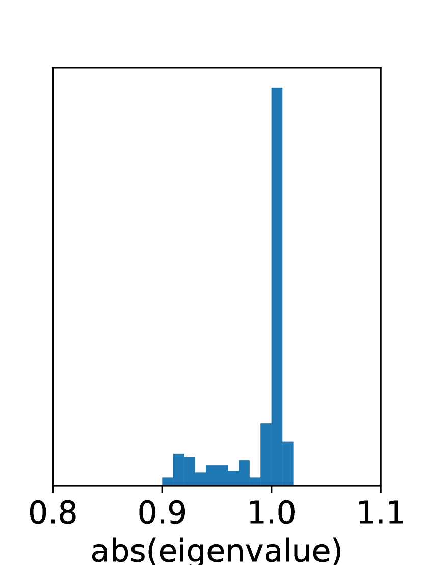
The linear constraint on dynamics stabilizes the training process, which is known to be unstable in standard recurrent NNs (see Section 3.3 and Fig. 6).
DBF has demonstrated superior performance over classical DA algorithms and latent assimilation methods in scenarios with highly non-Gaussian posteriors, particularly in the presence of strongly nonlinear observation operators or large observation noise.
2 Method
2.1 Inference of physical variables in a state-space model
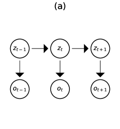
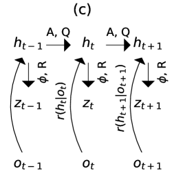
A physical system is defined by variables , with its evolution described by the dynamics model , where denotes a Gaussian whose mean and covariance are and . The nonlinear function is the dynamics operator and is the system covariance. The Markov property holds, as depends only on . An observation model relates observations to physical variables via the observation operator and covariance . The panel (a) of Fig. 1 shows the system’s graphical model. The objective of sequential DA is to compute the posterior of given .
2.2 KF for linear dynamics, linear observations
In the KF, the dynamics and observation models are both linear Gaussian, with the mean being linear with respect to the conditional variable and a constant covariance matrix. Given that the dynamics and observation operators are linear, we can represent them using matrices and , respectively. All matrices (, and ) are constant. The filter distribution remains Gaussian, provided that the initial distribution is Gaussian. We can recursively compute the posterior parameters (means and covariance matrices ) using the following equations:
| (1) | |||||
| (2) |
where is the Kalman Gain.
2.3 DBF for linear dynamics, nonlinear observations
In this scenario, Gaussianity of the test distribution is lost during the KF update step. We introduce an inverse observation operator (IOO) (see also Frerix et al. 2021):
| (3) |
where and is a virtual prior. By approximating both the IOO and the virtual prior as Gaussians, and , respectively, the posterior can be analytically computed as a Gaussian, where the mean and covariance are given as:
| (4) | |||||
| (5) |
where and are NNs with parameters , and and are constants set to and . These values bias the NNs’ outputs without affecting performance.
The recursive formula for the exact posterior (Equation 3) requires no approximation. Thus, DBF computes the exact posterior when the true IOO is Gaussian, i.e., the SSM is a LGSS. In that case, the posterior update formula agrees with the KF (see Equations 1, 2 and 4, 5). The key difference is that nonlinear functions are applied to both the mean, , and the covariance, . In the KF, is linear, and is a constant covariance matrix (see Equations 1 and 2). The dependence of on observations provides flexibility in adjusting the impact of the new observation on the state estimation. The importance of adjusting the internal state updates based on observations has also been discussed in recent SSM-based approaches (Gu & Dao, 2023).
2.4 DBF for nonlinear dynamics, linear/nonlinear observations
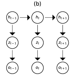
In this scenario, the Gaussianity of the test distribution is lost during the predict step, making it impossible to apply the original dynamics over the physical variables . Therefore, we introduce a new set of latent variables and assume a dynamics model over : (see panel (b) in Fig. 1). The IOO maps observations into the latent variables : . The recursive formula follows Equations 4 and 5. To retrieve the distribution of the original physical variables , we introduce an emission model , where is represented by a NN. By marginalizing over with this emission model, a trained DBF can generate samples of that follow the test distribution given observations .
Although the dynamics operator for the latent variables is linear, it is able to express any nonlinear dynamics if the latent space is sufficiently high-dimensional. The Koopman operator (Koopman, 1931) provides a framework for representing nonlinear systems by mapping observables—functions of the system’s state—into a higher-dimensional space where the dynamics become linear. Mathematically, for a dynamical system , the Koopman operator is a linear operator acting on a set of observables , such that . This allows the system to be represented as in the latent space , where is the dynamics matrix learned by DBF. While the physical dynamics are nonlinear, the Koopman operator ensures the existence of an embedding that linearizes the dynamics, enabling recursive computation of test distributions. Discovering such embeddings in finite dimensions has been widely studied (Takeishi et al., 2017; Lusch et al., 2018; Azencot et al., 2020). In high-dimensional simulations, the true degrees of freedom are often far fewer than the simulated variables, making surrogate modeling with the Koopman operator a promising approach to reducing computational costs.
2.5 Training
When assimilating in the physical space (i.e., when the dynamics are linear), we train the IOO (i.e., and ) by optimizing the evidence lower bound (ELBO) without using the teacher signal :
| (6) |
where denotes the Kullback-Leibler divergence between distributions and . If the SSM contains any unknown parameters, we can train these parameters as well.
For SSMs with nonlinear or unknown dynamics, we have two approaches:
Strategy 1
Pretrain the Koopman operator, which consists of the nonlinear mapping from to , the linear dynamics between and represented by matrix , and the reverse nonlinear mapping from to denoted by . With these components ( and ) of the Koopman operator, the method designed for linear dynamics can be applied. For pretraining, we require samples of or the SSM for the physical variables to generate these samples. Pairs of and are not necessary, as the training for the linear dynamics ( and ) and the IOO () can be performed separately.
Strategy 2
Train all components (the matrix , the stochastic mapping , and the IOO) simultaneously. In this case, samples of (, ) pairs or the SSM for both physical and observation variables to generate these sample pairs are required. The parameters are optimized by maximizing a joint ELBO, , via supervised training:
| (7) |
Here, we have neglected from . Since does not depend on and its distributions, it is sufficient to include . We have replaced with its special case as our objective is to give the best estimate of given observations .
2.6 Related works
We discuss related works in the order of relevance.
2.6.1 Dynamical variational autoencoders
DVAEs (see Girin et al. 2021 for a review) are models closely related to DBF for nonlinear dynamics. Both incorporate time-series architecture in a VAE, but there are two key differences: (i) the posterior design and realization of the dynamics step, and (ii) the loss function.
posterior design
Our strategy for the test distribution is to incorporate an appropriate architecture that reflects the Markov property in the time dimension of the test distribution. The IOO, , and the linear dynamics model serve as key instruments in constructing the test posterior distributions. A distinguishing feature of our methodology is that each component’s role is defined with respect to the Markov property of the state-space model (SSM) and is clearly differentiated from other components involved in posterior construction. For example, the IOO influences only the update step and does not affect the prediction step. We refer to this methodology as ”Bayes-Faithful” due to its tailored design for SSMs that exhibit the Markov property.
In contrast, the test posterior distributions in DVAEs are constructed using RNNs. The complexity of the transition model prevents the analytical computation of latent variables across time steps. As a result, these values can only be estimated via Monte Carlo sampling. Consequently, during inference, successive Monte Carlo sampling (“cascade trick”; Girin et al. 2021) becomes unavoidable.
loss function
DBF takes the ELBO from factorized density in :
| (8) |
On the other hand, DVAEs take the ELBO from probability density with all the observations at once.
| (9) |
Therefore, DBF seeks for the filtered distributions whereas DVAEs model the smoother distributions . Again, for DVAEs, to evaluate the expected values in Equation 9, we need to undergo successive Monte-Carlo sampling over variables ().
Assuming linear Gaussian dynamics and a Gaussian IOO, DBF allows for the analytical integration of , resulting in a structured encoder. This structured posterior enables the recursive computation of the filtered distribution without relying on Monte Carlo sampling, setting it apart from other DVAEs. By constraining the dynamics to be linear, DBF ensures exact integration without the accumulation of Monte Carlo sampling errors across time steps.
Moreover, the linear assumption helps DBF mitigate the instability issues commonly faced when training standard RNNs. SSMs are increasingly favored for modeling long-range dependencies (Gu & Dao, 2023). S4 (Gu et al., 2022) utilizes linear dynamics in the latent space and learns the dynamics, proposing an efficient computation algorithm that outperforms transformers on datasets with long-range dependencies. LS4 (Zhou et al., 2023) extends S4 by introducing stochasticity through a VAE-like structure. Both LS4 and DBF employ linear SSMs and Gaussian posterior approximations, but DBF updates the mean and covariance using a recursive formula based on Bayes’ rule, while LS4 replaces recurrence with convolutions, forgoing a recursive approach.
2.6.2 KF-based methods
Various approaches have been explored to address LGSS limitations, including linearizing the model via first-order approximations like the extended Kalman Filter (EKF), approximating populations with a Gaussian distribution in the ensemble Kalman Filter (EnKF; Evensen 1994), and using NNs to approximate the Kalman gain (Revach et al., 2022). The EnKF and its variants (e.g., ETKF; Bishop et al. 2001) are commonly used in real-time data assimilation for weather forecasting. However, these methods rely on the KF’s posterior update equations, limiting the expressivity of the distributions they can represent. Additionally, computations for covariance matrices become challenging in high-dimensional spaces, requiring specialized techniques for computational efficiency.
2.6.3 Sampling-based methods
The Particle Filter is a popular method for assimilating any posterior. However, achieving adequate particle density in high-dimensional state spaces poses significant challenges. Insufficient density of particles leads to particle degeneracy, where few particles explain the observed data (Beskos et al., 2014). In contrast, DBF directly learns to position density through the IOO, offering advantages for high-dimensional tasks. The Particle Flow Filter (PFF; Daum & Huang 2007; Hu & van Leeuwen 2021) addresses particle degeneracy by moving particles according to gradient flow and effectively scales to nonlinear SSMs with hidden state dimensions up to 1000 (Hu & van Leeuwen, 2021).
2.6.4 Approximate MAP estimation method
MAP estimation is used to identify the high-density point of the posterior in high-dimensional space, such as in weather forecasting Lorenc (2003); Frerix et al. (2021). Even if the computation of the posterior is intractable, we can optimize if we can describe and explicitly. In practice, we cannot access and therefore the integral , so we only compute the mean. The downside is that sequential computation of the covariance matrix of is impossible.
2.6.5 NN-based PDE surrogate
Recently, there have been attempts to approximate partial differential equations (PDEs) using NNs. We also tried one of the latest methods, PDE-refiner (Lippe et al., 2023), in the experiments of this study. However, its performance was poor, and we decided not to include it in the experiments. We suspect this is because PDE-refiner was designed for constructing PDE surrogates and did not account for noisy observations, making it susceptible to noise. We confirmed that it produces good predictions under noiseless observations.
3 Experiments
We evaluate the performance of DBF on three tasks: a linear dynamics problem (moving MNIST) and two nonlinear dynamics problems (double pendulum and Lorenz96).
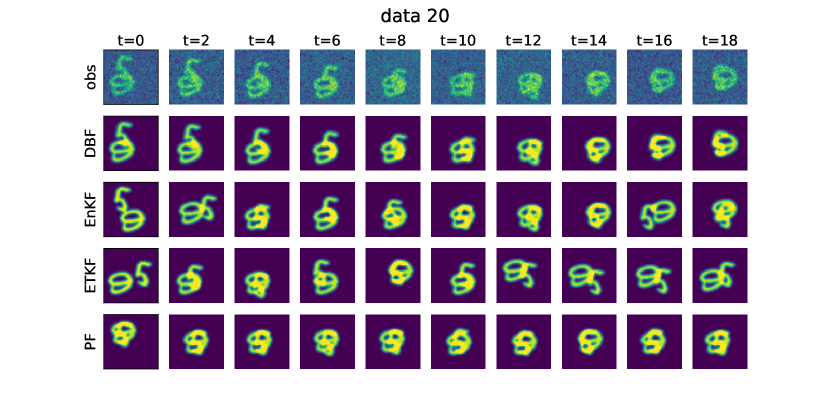
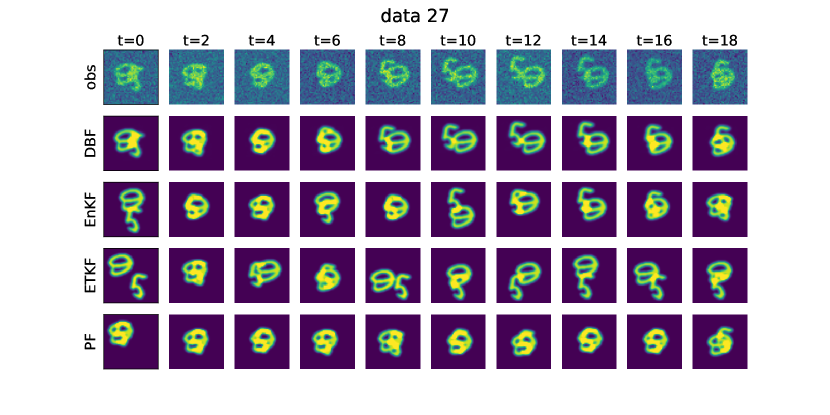
Linear dynamics: moving MNIST
In the moving MNIST task, the goal is to identify the images, positions, and velocities of two handwritten digits as they move within the observed frames. While the dynamics of these digit images and their observation processes are provided, the actual images, positions, and velocities are not available, making supervised learning impossible. DBF assimilates directly in the physical space. It trains the parameters of the IOO, and , which are represented by NNs, along with the pixel values of the embedded images. The results are compared against conventional DA methods (EnKF, ETKF, PF) that also operate in the physical space.
Nonlinear dynamics: double pendulum and Lorenz96
For nonlinear dynamics problems, such as the double pendulum and Lorenz96, DBF constructs a new latent space in addition to the original physical space. Here, we took Strategy 2 in Sec.2.5 for the training: we simultaneously train NNs for the IOO, nonlinear observation operator , the dynamics matrix , and the emission model’s standard deviation. We compare the performance of DBF with the classical DA algorithms (EnKF, ETKF, PF), state-of-the-art assimilation methodologies (PFF Daum & Huang 2007; Hu & van Leeuwen 2021, KalmanNet Revach et al. 2022), and DVAE-based approaches (deep Kalman Filter; DKF, Krishnan et al. 2015; 2016, variational recurrent neural network; VRNN, Chung et al. 2015, and stochastic recurrent neural network; SRNN, Fraccaro et al. 2016). DBF and other DVAEs are trained by optimizing the evidence lower bound (ELBO), as described in Sec. 2.5.
For all the experiments, we generate random initial conditions and let them evolve via the dynamics of the problem. Synthetic observation data are generated by applying the observation operator and additive noise. Noise levels and observation operators are further explained in the section for each problem and in the appendix. Training details, including hyperparameters and architectures, are also provided in the appendix.
3.1 Linear dynamics: two-body moving MNIST
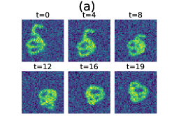
This experiment demonstrates DBF’s ability to handle linear dynamics where key parameters of the observation operator are unknown. The dataset consists of 2D figures containing two embedded images, each moving at a constant speed and bouncing off frame edges. The system’s physical state is described by eight variables: the positions and velocities of the two embedded images. The dynamics matrix is block-diagonal, composed of four (two-body times two dimensions) translation matrices, : . Observations are corrupted by additive Gaussian noise with a standard deviation of per pixel, where the original pixel values range from to (see panel (a) of Fig. 2 for an example of the data provided).
The aim is to show that DBF can track the linear dynamics while estimating unknown system parameters. DBF learns the pixel values of the embedded images from noisy observations, while maintaining consistency with physical motion. The observation model contains unknown parameters, corresponding to the number of pixels in the images. In classical DA algorithms, it is not possible to train unknown system parameters. However, it may be possible to infer these parameters by incorporating them as new physical dimensions. We have adopted this strategy for classical DA algorithms (EnKF, ETKF, and PF). We tested at three different noise levels ( of , , and ). DVAEs are not comparable as they need to undergo supervised training. We were unable to compare with KalmanNet, as its input dimensionality, , exceeded the available GPU memory.
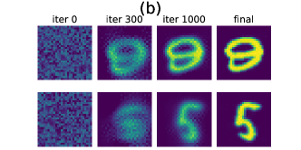
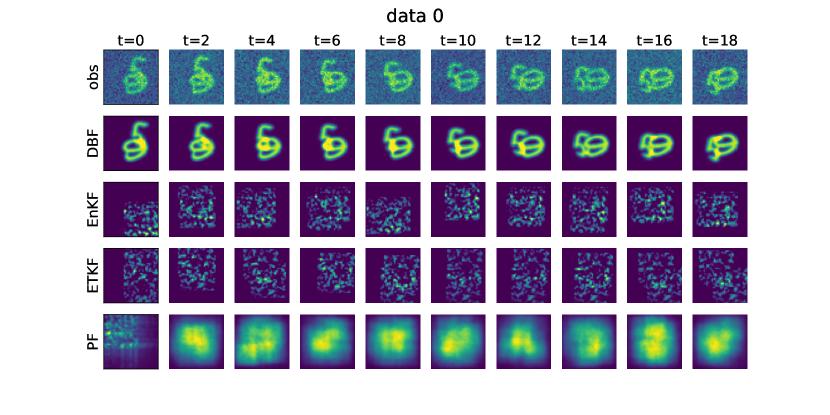
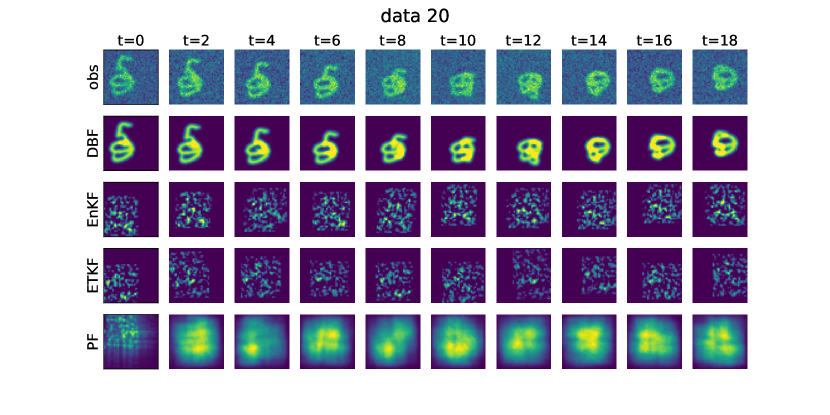
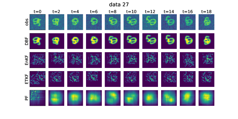
Fig. 2 summarizes the experiment. Panel (a) shows an example from the test set, illustrating the challenges posed by strong noise and overlapping images. Panel (b) presents the DBF learning process. In the rightmost table, we compare the success rates of DBF against model-based approaches (EnKF, ETKF, PF). We define success as achieving a root-mean-square error (RMSE) of less than 1.0 for both position () and velocity () of the two digits over the final ten steps. DBF successfully performs assimilation without explicit knowledge of the images, while all the other model-based approaches fail. The KF-inspired approaches (EnKF, ETKF) failed because of very strong non-Gaussianity in the observation process and the high system dimension. Similarly, PF underperformed because the number of particles () was insufficient for the problem dimension ( and two digits images ). Figures for visualizing the assimilation results for all the algorithms are given in the appendix (Fig. 7).
Panel (b) of Fig. 2 illustrates the evolution of the estimated figures. Initially, DBF assumes two random shapes. As training progresses, it first identifies one of the numbers (“9”) and subsequently detects the second shape (“5”). By the end of the training process, DBF nearly perfectly estimates the parameters of the observation model, including the positions of the figures, which is crucial for adjusting their reflective behavior. The ability to learn system parameters through gradient descent sets DBF apart from traditional model-based approaches.
| Method | Success rate |
|---|---|
| DBF | 100% (50/50) |
| EnKF | 0% (0/50) |
| ETKF | 0% (0/50) |
| PF | 0% (0/50) |
3.2 Nonlinear dynamics 1: double pendulum
| KLsym | |
|---|---|
| DBF | 0.02 |
| EnKF | 10.2 |
| ETKF | 0.12 |
| DBF | 0.03 0.01 | 0.21 0.04 | 0.05 0.02 | 0.26 0.05 | 0.06 0.01 | 0.36 0.04 |
|---|---|---|---|---|---|---|
| EnKF | ||||||
| ETKF | ||||||
| PF | ||||||
| PFF | NA | NA | ||||
| KNet | NA | NA | NA | NA | NA | NA |
| VRNN | ||||||
| SRNN | ||||||
| DKF | ||||||
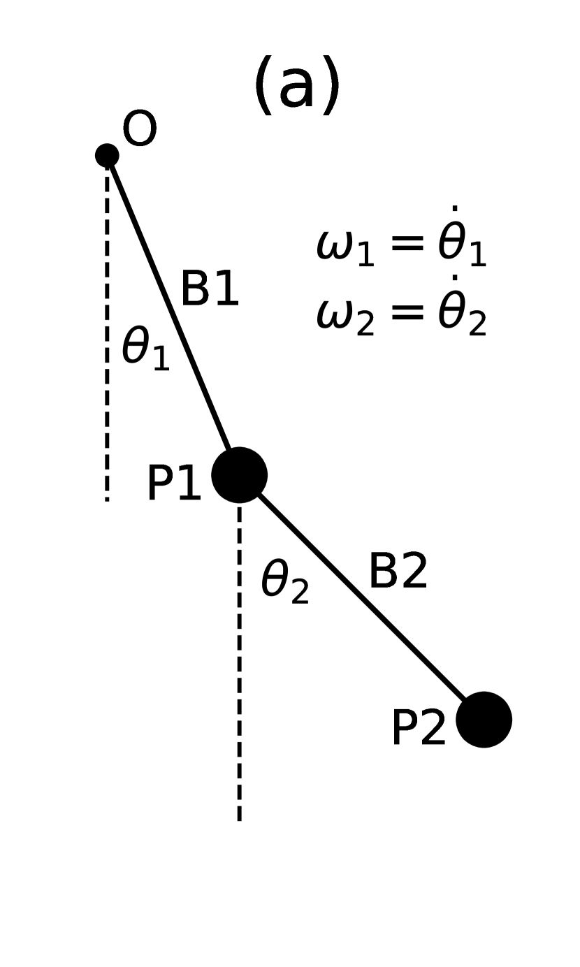
This section presents our experiments with a double pendulum system, selected for its nonlinear and chaotic behavior. The pendulum consists of two 1 kg masses, P1 and P2, connected by two 1 meter bars, B1 and B2. One end of the bar B1 is fixed at the origin (“O”), with the other end attached to P1. Mass P2 is connected to P1 via bar B2. A schematic of the setup is shown in panel (a) of Fig. 3.
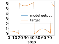
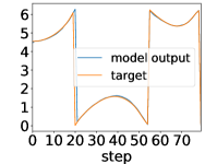
We use the angles and , and the two angular velocities, and , as target physical variables. The latent dimension for DBF, VRNN, SRNN, and DKF is set to 50. Observation data consists of the two-dimensional spatial positions of masses and , corrupted by Gaussian noise. The observation operator combines trigonometric functions for and , creating a highly nonlinear relationship. Experiments are conducted with noise levels of , and meters, with a time step of 0.03 seconds between observations. In the emission model , we assume von Mises distributions for and , while and follow Gaussian distributions.
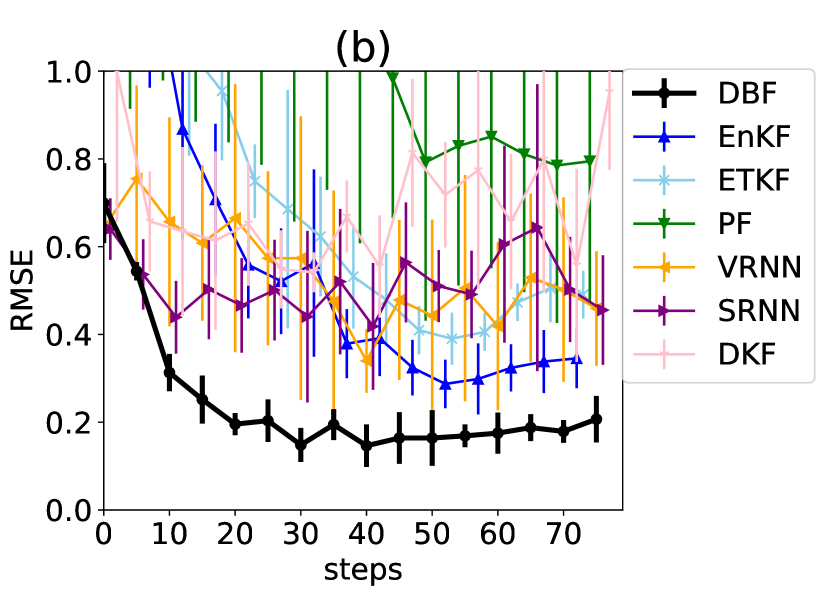
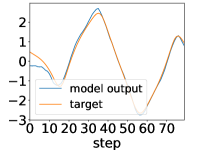
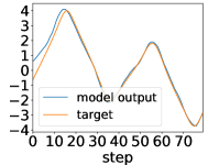
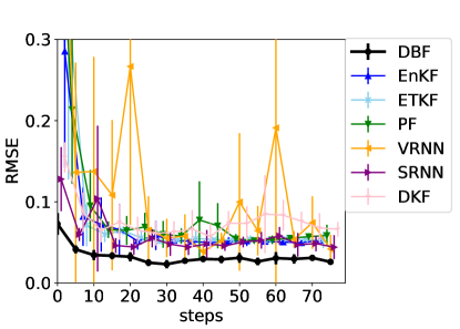
Table 1 presents the RMSE between the physical variables and the mean of the filtered distribution. Training for KalmanNet was unsuccessful under all conditions. For the DVAEs, we exclude failed initial conditions when calculating the RMSE. DBF outperforms both model-based and latent assimilation methods across all settings, showing significant improvements in estimating , which cannot be inferred from a single observation. Fig. 3 (b) illustrates an example of RMSE evolution during assimilation, where DBF consistently outperforms the other methods. The assimilation of occurs within the first steps, maintaining an excellent estimation accuracy throughout the experiment.
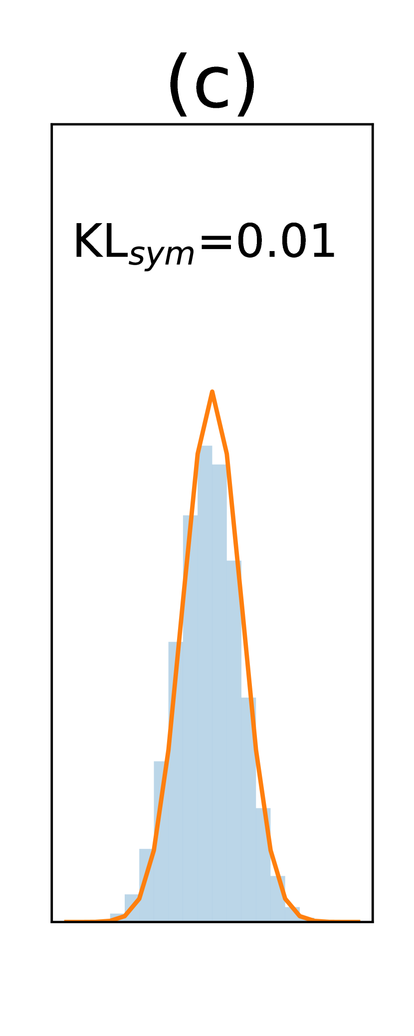
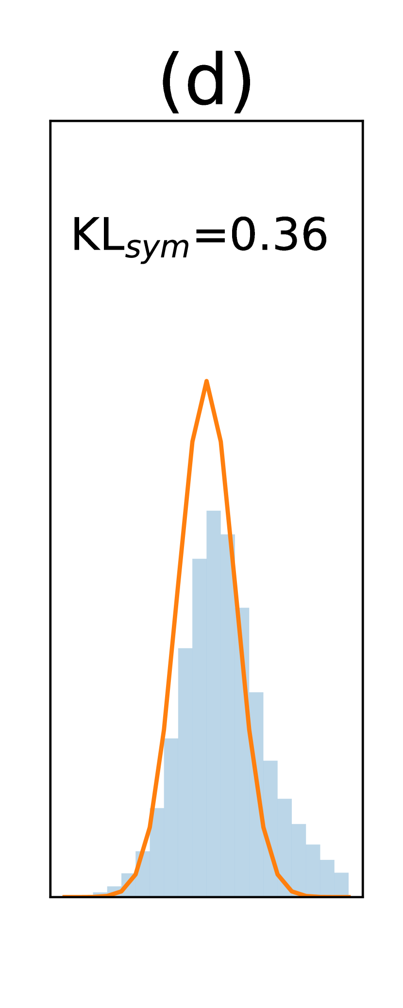
A key feature of DBF is its ability to generate samples of and assess the uncertainty in state estimates. To evaluate this capability, we analyze the distributions of normalized errors defined as , where represents the true value of dimension at time , and is the standard deviation of . We collect across all time steps, focusing on and , since and follow von Mises distributions. If the uncertainty estimates are accurate, should approximate a Gaussian distribution with a standard deviation of one. To quantify the accuracy, we compute the symmetric KL divergence (Jeffreys divergence) between the histogram of and a unit Gaussian. DBF exhibits very low values, indicating accurate error estimation. Panels (c) and (d) display example histograms of for DBF and ETKF.
3.3 Nonlinear dynamics 2: Lorenz96
In the final experiment, we focus on state estimation in the Lorenz96 model (Lorenz, 1995), a benchmark for testing data assimilation algorithms on noisy, nonlinear observations. The Lorenz96 model describes the evolution of a one-dimensional array of variables, each representing a physical quantity over a spatial domain, like an equilatitude circle. The dynamics are governed by the following coupled ordinary differential equations:
| (10) |
where is the value at grid point , is the number of grid points, and is external forcing. For our experiments, we take and .
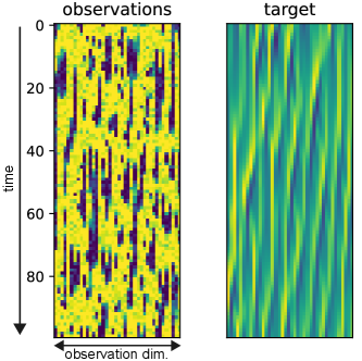
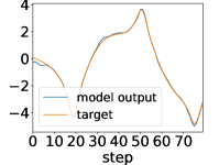
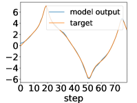
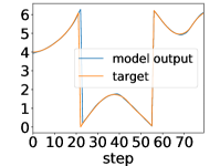
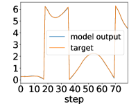
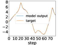
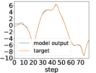
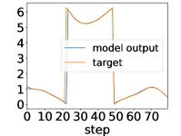
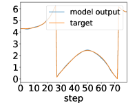
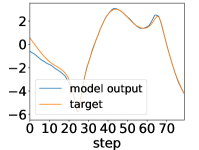
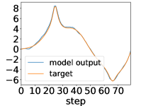
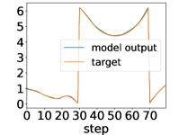
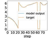
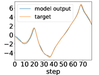
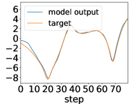
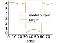
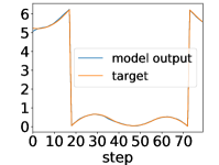
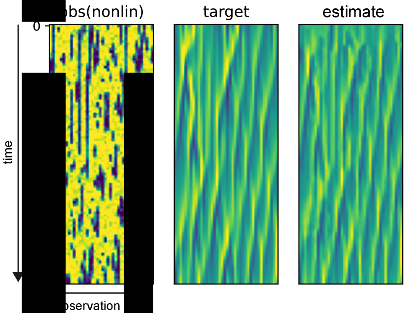
We consider two observation operators. The first adds Gaussian noise to direct observations: , with noise levels . The second uses a nonlinear operator: , with the same noise levels. The dynamic range of is around , and observations are capped at 10 when exceeds 1.8. This makes it highly challenging for classical DA methods, as each observation offers limited information. The filter must integrate data over long timesteps, where nonlinear dynamics distort the probability distribution. Fig. 4 illustrates observations and target values. All models use 80 observation steps with a 0.03 time interval. The latent dimension for DBF, VRNN, SRNN, and DKF is set to 800. For further details for the experiment, see Sec. A.3.
| direct observation | nonlinear observation | |||||
| DBF | 0.82 0.03 | 1.16 0.07 | 1.08 0.15 | 1.29 0.18 | 1.65 0.17 | |
| EnKF | ||||||
| ETKF | 0.30 0.01 | |||||
| PF | ||||||
| PFF | ||||||
| KNet | ||||||
| VRNN | ||||||
| SRNN | ||||||
| DKF | 3.70 | NA | NA | NA | NA | NA |
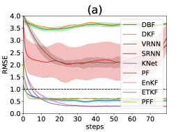
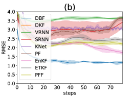
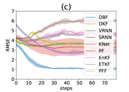
Table 2 presents the assimilation performance across different noise levels and observation settings. DBF outperforms existing methods in direct observations with , and across all noise levels for nonlinear observation cases. In the setting with direct observation, traditional algorithms like EnKF and ETKF outperform DBF.
The superior performance of EnKF and ETKF with direct observations at the lowest noise level can be attributed to the minimal non-Gaussianity in the posteriors within physical space. Non-Gaussianity can originate from both the dynamics model (predict step) and the observation model (update step). In this setting, the linearity of the observation operator prevents non-Gaussianity from being introduced during the update step, provided that the prior is Gaussian. Additionally, state estimation from each observation is highly accurate due to small noise. As a result, the prior remains close to a Gaussian distribution, as the locally linear approximation of the dynamics adequately captures the time evolution of probability distributions. The poorer performance of EnKF and ETKF in the experiment is attributed to the increased non-Gaussianity introduced during each predict step. Similarly, when the observation operator is nonlinear, each update step introduces substantial non-Gaussianity. This results in a significant drop in performance for traditional filtering methods across all noise levels. In these scenarios, DBF consistently maintains an advantage over classical DA algorithms.
| setting | max[abs(eig)] |
|---|---|
| D, | |
| D, | |
| D, | |
| N, | |
| N, | |
| N, |
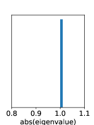
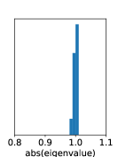
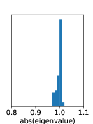
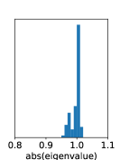
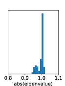
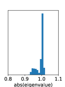
We observe that training DVAE-based methods is highly unstable, while that for DBF exhibits stability. Dynamics in DVAEs are modeled by RNNs, which often suffer from unstable training due to exploding or vanishing gradients. In contrast, DBF employs matrix multiplication for dynamics. If the eigenvalues of the matrix exceed one by a large margin, the model predictions, and consequently the loss function, would explode irrespective of inputs. Fig. 6 shows the histogram of the absolute values of eigenvalues at the end of training, which are distributed around or below one, indicating stable training.
4 Limitation
DBF’s learning of IOO requires a training phase, unlike classical model-based data assimilation methods. Specifically, when dealing with nonlinear dynamics, DBF requires either: (i) a pair of generated from the original SSM, (ii) a pair of obtained via, e.g., retrospective reanalysis (ERA5; Hersbach et al. 2020 in weather forecasting), or (iii) a pretrained Koopman operator and observed data .
In the Lorenz96 experiment, DBF’s performance with direct observation with falls short compared to EnKF and ETKF. In this setting, the non-Gaussianity of posteriors is weak, resulting in minor approximation errors due to Gaussian assumptions. Consequently, a model-based approach may be more advantageous in such situations, as it leverages complete SSM knowledge without introducing training biases.
5 Conclusion
We propose DBF, a novel DA method. DBF is a NN-based extension of the KF designed to handle nonlinear observations. While constraining the test distributions to remain Gaussian, DBF enhances their representational capacity by leveraging nonlinear transform expressed by a NN. DBF is the first “Bayes-Faithful” amortized variational inference methodology, constructing test distributions that mirror the inference structure of a SSM with the Markov property. This structured inference enables analytical computation of test distributions, preventing the accumulation of Monte Carlo sampling errors over time steps. DBF exhibits superior performance over existing methods in scenarios where posterior distributions become highly non-Gaussian, such as in the presence of nonlinear observation operators or significant observation noise.
References
- Alfonzo & Oliver (2020) Miguel Alfonzo and Dean S. Oliver. Seismic data assimilation with an imperfect model. Computational Geosciences, 24(2):889–905, 2020. Marine Environmental Monitoring and Prediction.
- Andrychowicz et al. (2023) Marcin Andrychowicz, Lasse Espeholt, Di Li, Samier Merchant, Alexander Merose, Fred Zyda, Shreya Agrawal, and Nal Kalchbrenner. Deep learning for day forecasts from sparse observations. ArXiv, abs/2306.06079, 2023. URL https://api.semanticscholar.org/CorpusID:259129311.
- Awal et al. (2023) Md Abdul Awal, Md Abu Rumman Refat, Feroza Naznin, and Md Zahidul Islam. A particle filter based visual object tracking: A systematic review of current trends and research challenges. International Journal of Advanced Computer Science and Applications, 14(11), 2023. doi: 10.14569/IJACSA.2023.01411131. URL http://dx.doi.org/10.14569/IJACSA.2023.01411131.
- Azencot et al. (2020) Omri Azencot, N. Benjamin Erichson, Vanessa Lin, and Michael Mahoney. Forecasting sequential data using consistent koopman autoencoders. In Hal Daumé III and Aarti Singh (eds.), Proceedings of the 37th International Conference on Machine Learning, volume 119 of Proceedings of Machine Learning Research, pp. 475–485. PMLR, 13–18 Jul 2020. URL https://proceedings.mlr.press/v119/azencot20a.html.
- Bach & Ghil (2023) Eviatar Bach and Michael Ghil. A multi-model ensemble kalman filter for data assimilation and forecasting. Journal of Advances in Modeling Earth Systems, 15(1):e2022MS003123, 2023. doi: https://doi.org/10.1029/2022MS003123. URL https://agupubs.onlinelibrary.wiley.com/doi/abs/10.1029/2022MS003123. e2022MS003123 2022MS003123.
- Beskos et al. (2014) Alexandros Beskos, Dan Crisan, and Ajay Jasra. On the stability of sequential Monte Carlo methods in high dimensions. The Annals of Applied Probability, 24(4):1396 – 1445, 2014. doi: 10.1214/13-AAP951. URL https://doi.org/10.1214/13-AAP951.
- Bishop et al. (2001) Craig H. Bishop, Brian J. Etherton, and Sharanya J. Majumdar. Adaptive Sampling with the Ensemble Transform Kalman Filter. Part I: Theoretical Aspects. Mon. Wea. Rev., 129(3):420–436, March 2001. ISSN 0027-0644, 1520-0493. doi: 10.1175/1520-0493(2001)129¡0420:ASWTET¿2.0.CO;2. URL http://journals.ametsoc.org/doi/10.1175/1520-0493(2001)129<0420:ASWTET>2.0.CO;2.
- Chopin & Papaspiliopoulos (2020) Nicolas Chopin and Omiros Papaspiliopoulos. An introduction to Sequential Monte Carlo. Springer series in statistics. Springer, 2020. URL https://ci.nii.ac.jp/ncid/BC03234800.
- Chung et al. (2015) Junyoung Chung, Kyle Kastner, Laurent Dinh, Kratarth Goel, Aaron C Courville, and Yoshua Bengio. A Recurrent Latent Variable Model for Sequential Data. In Advances in Neural Information Processing Systems, volume 28. Curran Associates, Inc., 2015. URL https://proceedings.neurips.cc/paper_files/paper/2015/hash/b618c3210e934362ac261db280128c22-Abstract.html.
- Daum & Huang (2007) Fred Daum and Jim Huang. Nonlinear filters with log-homotopy. In Oliver E. Drummond and Richard D. Teichgraeber (eds.), Signal and Data Processing of Small Targets 2007, volume 6699, pp. 669918. International Society for Optics and Photonics, SPIE, 2007. doi: 10.1117/12.725684. URL https://doi.org/10.1117/12.725684.
- Evensen (1994) Geir Evensen. Sequential data assimilation with a nonlinear quasi-geostrophic model using Monte Carlo methods to forecast error statistics. Journal of Geophysical Research: Oceans, 99(C5):10143–10162, 1994. ISSN 2156-2202. doi: 10.1029/94JC00572. URL https://onlinelibrary.wiley.com/doi/abs/10.1029/94JC00572. _eprint: https://onlinelibrary.wiley.com/doi/pdf/10.1029/94JC00572.
- Fraccaro et al. (2016) Marco Fraccaro, Søren Kaae Sønderby, Ulrich Paquet, and Ole Winther. Sequential neural models with stochastic layers. In Proceedings of the 30th International Conference on Neural Information Processing Systems, NIPS’16, pp. 2207–2215, Red Hook, NY, USA, 2016. Curran Associates Inc. ISBN 978-1-5108-3881-9.
- Frerix et al. (2021) Thomas Frerix, Dmitrii Kochkov, Jamie Smith, Daniel Cremers, Michael Brenner, and Stephan Hoyer. Variational Data Assimilation with a Learned Inverse Observation Operator. In Proceedings of the 38th International Conference on Machine Learning, pp. 3449–3458. PMLR, July 2021. URL https://proceedings.mlr.press/v139/frerix21a.html. ISSN: 2640-3498.
- Girin et al. (2021) Laurent Girin, Simon Leglaive, Xiaoyu Bie, Julien Diard, Thomas Hueber, and Xavier Alameda-Pineda. Dynamical variational autoencoders: A comprehensive review. Foundations and Trends® in Machine Learning, 15(1-2):1–175, 2021. ISSN 1935-8237. doi: 10.1561/2200000089. URL http://dx.doi.org/10.1561/2200000089.
- Gu & Dao (2023) Albert Gu and Tri Dao. Mamba: Linear-time sequence modeling with selective state spaces. arXiv preprint arXiv:2312.00752, 2023.
- Gu et al. (2022) Albert Gu, Karan Goel, and Christopher Re. Efficiently modeling long sequences with structured state spaces. In International Conference on Learning Representations, 2022. URL https://openreview.net/forum?id=uYLFoz1vlAC.
- Hersbach et al. (2020) Hans Hersbach, Bill Bell, Paul Berrisford, Shoji Hirahara, András Horányi, Joaquín Muñoz-Sabater, Julien Nicolas, Carole Peubey, Raluca Radu, Dinand Schepers, Adrian Simmons, Cornel Soci, Saleh Abdalla, Xavier Abellan, Gianpaolo Balsamo, Peter Bechtold, Gionata Biavati, Jean Bidlot, Massimo Bonavita, Giovanna De Chiara, Per Dahlgren, Dick Dee, Michail Diamantakis, Rossana Dragani, Johannes Flemming, Richard Forbes, Manuel Fuentes, Alan Geer, Leo Haimberger, Sean Healy, Robin J. Hogan, Elías Hólm, Marta Janisková, Sarah Keeley, Patrick Laloyaux, Philippe Lopez, Cristina Lupu, Gabor Radnoti, Patricia de Rosnay, Iryna Rozum, Freja Vamborg, Sebastien Villaume, and Jean-Noël Thépaut. The era5 global reanalysis. Quarterly Journal of the Royal Meteorological Society, 146(730):1999–2049, 2020. doi: https://doi.org/10.1002/qj.3803. URL https://rmets.onlinelibrary.wiley.com/doi/abs/10.1002/qj.3803.
- Hu & van Leeuwen (2021) Chih-Chi Hu and Peter Jan van Leeuwen. A particle flow filter for high-dimensional system applications. Quarterly Journal of the Royal Meteorological Society, 147(737):2352–2374, 2021. doi: https://doi.org/10.1002/qj.4028. URL https://rmets.onlinelibrary.wiley.com/doi/abs/10.1002/qj.4028.
- Hunt et al. (2007) Brian R. Hunt, Eric J. Kostelich, and Istvan Szunyogh. Efficient data assimilation for spatiotemporal chaos: A local ensemble transform kalman filter. Physica D: Nonlinear Phenomena, 230(1):112–126, 2007. ISSN 0167-2789. doi: https://doi.org/10.1016/j.physd.2006.11.008. URL https://www.sciencedirect.com/science/article/pii/S0167278906004647. Data Assimilation.
- Koopman (1931) B. O. Koopman. Hamiltonian systems and transformation in hilbert space. Proceedings of the National Academy of Sciences, 17(5):315–318, 1931. doi: 10.1073/pnas.17.5.315. URL https://www.pnas.org/doi/abs/10.1073/pnas.17.5.315.
- Krishnan et al. (2015) Rahul G. Krishnan, Uri Shalit, and David Sontag. Deep kalman filters, 2015. URL https://arxiv.org/abs/1511.05121.
- Krishnan et al. (2016) Rahul G. Krishnan, Uri Shalit, and David Sontag. Structured inference networks for nonlinear state space models, 2016. URL https://arxiv.org/abs/1609.09869.
- Larsen et al. (2007) J. Larsen, J.L. Høyer, and J. She. Validation of a hybrid optimal interpolation and kalman filter scheme for sea surface temperature assimilation. Journal of Marine Systems, 65(1):122–133, 2007. ISSN 0924-7963. doi: https://doi.org/10.1016/j.jmarsys.2005.09.013. URL https://www.sciencedirect.com/science/article/pii/S0924796306002880. Marine Environmental Monitoring and Prediction.
- Lippe et al. (2023) Phillip Lippe, Bastiaan S. Veeling, Paris Perdikaris, Richard E Turner, and Johannes Brandstetter. PDE-Refiner: Achieving Accurate Long Rollouts with Temporal Neural PDE Solvers. In Thirty-seventh Conference on Neural Information Processing Systems, 2023. URL https://openreview.net/forum?id=Qv6468llWS.
- Lorenc (2003) Andrew C. Lorenc. Modelling of error covariances by 4d-var data assimilation. Quarterly Journal of the Royal Meteorological Society, 129(595):3167–3182, 2003. doi: https://doi.org/10.1256/qj.02.131. URL https://rmets.onlinelibrary.wiley.com/doi/abs/10.1256/qj.02.131.
- Lorenz (1995) E.N. Lorenz. Predictability: a problem partly solved. PhD thesis, Shinfield Park, Reading, 1995 1995.
- Lusch et al. (2018) Bethany Lusch, J. Nathan Kutz, and Steven L. Brunton. Deep learning for universal linear embeddings of nonlinear dynamics. Nature Communications, 9:4950, November 2018. doi: 10.1038/s41467-018-07210-0.
- Ohishi et al. (2024) Shun Ohishi, Takemasa Miyoshi, Takafusa Ando, Tomohiko Higashiuwatoko, Eri Yoshizawa, Hiroshi Murakami, and Misako Kachi. Letkf-based ocean research analysis (lora) version 1.0. Geoscience Data Journal, n/a(n/a), 2024. doi: https://doi.org/10.1002/gdj3.271. URL https://rmets.onlinelibrary.wiley.com/doi/abs/10.1002/gdj3.271.
- Revach et al. (2022) Guy Revach, Nir Shlezinger, Xiaoyong Ni, Adrià López Escoriza, Ruud J. G. van Sloun, and Yonina C. Eldar. Kalmannet: Neural network aided kalman filtering for partially known dynamics. IEEE Transactions on Signal Processing, 70:1532–1547, 2022. doi: 10.1109/TSP.2022.3158588.
- Takeishi et al. (2017) Naoya Takeishi, Yoshinobu Kawahara, and Takehisa Yairi. Learning koopman invariant subspaces for dynamic mode decomposition. In I. Guyon, U. Von Luxburg, S. Bengio, H. Wallach, R. Fergus, S. Vishwanathan, and R. Garnett (eds.), Advances in Neural Information Processing Systems, volume 30. Curran Associates, Inc., 2017. URL https://proceedings.neurips.cc/paper_files/paper/2017/file/3a835d3215755c435ef4fe9965a3f2a0-Paper.pdf.
- Zhou et al. (2023) Linqi Zhou, Michael Poli, Winnie Xu, Stefano Massaroli, and Stefano Ermon. Deep latent state space models for time-series generation. In Andreas Krause, Emma Brunskill, Kyunghyun Cho, Barbara Engelhardt, Sivan Sabato, and Jonathan Scarlett (eds.), International Conference on Machine Learning, ICML 2023, 23-29 July 2023, Honolulu, Hawaii, USA, volume 202 of Proceedings of Machine Learning Research, pp. 42625–42643. PMLR, 2023. URL https://proceedings.mlr.press/v202/zhou23i.html.
Appendix A Settings and additional results for experiments
parametrization of the dynamics matrix
We have parametrized the dynamics matrix following Lusch et al. (2018): we consider that complex eigenvalues characterize . Namely, is a block-diagonal matrix of blocks. Each block consists of matrix, whose components are:
| (11) |
where and . In contrast to Lusch et al. (2018), we apply the same dynamics matrix at any positions on the latent space. We consider that this representation is sufficiently expressive, as it can express any matrix on a complex number field that is diagonalizable.
One key advantage of DBF is that augmenting the latent dimension only results in a linear increase in computational demand. This scaling is due to the efficient parametrization of the dynamics matrix, where the block-diagonal structure allows operations to scale linearly with the latent dimension. In contrast, methods such as Sequential Monte Carlo (SMC) suffer from exponential increases in computational demand as the latent space grows, assuming that the same density of particles must be maintained to capture posterior distributions. This makes DBF particularly well-suited for high-dimensional systems where traditional methods struggle with computational complexity.
Computational resources
We conduct experiments on a cluster of V100 GPUs. Each GPU has memory of 32GB.
hyperparameters for training
For all experiments, we have used Adam optimizer with default parameters. Table 3 shows hyperparameters employed in our experiments. Trainings for moving MNIST and double pendulum are conducted with one GPU, while that for Lorenz96 is with eight GPUs.
| lr | batch size | Epochs | train time per model | |||
|---|---|---|---|---|---|---|
| moving MNIST | 64 | 8 | 480,000 | 2 | 3hr 1GPU | |
| double pendulum | 256 | 50 | 1 | 6hr 1GPU | ||
| Lorenz96 | 64 | 800 | 1 | 15hr 8GPUs |
A.1 Moving MNIST
Dataset:
The dataset consists of a series of 2D images, where each pixel has a dynamic range from 0 to 255. The training set contains initial conditions, while the test set consists of ten initial conditions, with both datasets comprising 20 time steps each. The number of training samples and epochs is sufficiently large to ensure that the training converges effectively. A Gaussian noise with a standard deviation of is added to all pixels. The MNIST images of the digits “9” (data point 5740) and “5” (data point 5742) move at constant speeds until they reach the edges, where reflection occurs.
Training:
The network weights for are fixed during the first epoch to facilitate the learning of and the image tensor for the observation model. Subsequently, is trained during the second epoch. In total, DBF undergoes training for two epochs.
Dynamics model:
Constant velocity model. The exact dynamics matrix we have used is:
| (12) |
| (13) |
and true observation model:
| (14) | |||||
| (15) |
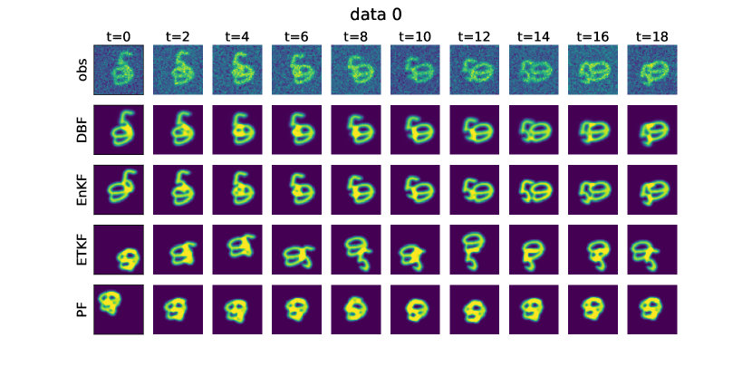
The formulation above addresses image reflection through the observation operator, resulting in linear dynamics while permitting multiple solutions for each observed figure. This approach presents significant challenges for the EnKF, which assumes a single-peak Gaussian distribution in the assimilating space. To ensure a fair comparison, we revise the dynamics and observation models to allow for a single solution for each figure. This adjustment notably enhances the performance of the EnKF if the image is provided. However, even with this modification, the EnKF fails to accurately estimate the position, velocity, and the embedded image.
Network architecture:
: Two-dimension convolutional NNs. Below is the list of layers.
-
•
conv1: nn.Conv2d(1, 2, kernel_size=3, stride=2, padding=1)
-
•
conv2: nn.Conv2d(2, 4, kernel_size=3, stride=2, padding=1)
-
•
conv3: nn.Conv2d(4, 4, kernel_size=3, stride=1, padding=1)
-
•
conv4: nn.Conv2d(4, 4, kernel_size=3, stride=1, padding=1)
-
•
fc: nn.Linear(, 8)
The input image, sized , is sequentially processed by convolutional layers (conv1, conv2, conv3, and conv4). The output is then flattened to serve as the input for the fully connected layer (fc). Ultimately, this process yields eight variables for . The network follows the same architecture as , but it produces only the diagonal components of through the NN.
| parameter | value |
|---|---|
| diag[] | |
| diag[] |
Example figures:
In Fig. 8, we show example images for observations and all the algorithms in image-informed setting.
| Method | Success rate |
|---|---|
| DBF | 100% (50/50) |
| EnKF | 58% (29/50) |
| ETKF | 0% (0/50) |
| PF | 0% (0/50) |
A.2 Double pendulum
Dataset:
The dataset consists of 2D coordinates representing the positions of two weights. The training set includes initial conditions, while the test set contains 10 initial conditions. The number of training samples is sufficiently large to ensure that the training converges. During DVAE training, we observed that some initial conditions resulted in training failure due to instability; however, we maintained the total number of training samples since the training was successful for at least one initial condition. Both datasets comprise 80 time steps. Numerical integration is performed using the solve_ivp function in SciPy, with relative tolerance (rtol) set to and absolute tolerance (atol) set to .
A schematic figure explaining the problem setting is presented in panel (a) of Fig. 3 in the main text.
Dynamics model is described in https://matplotlib.org/stable/gallery/animation/double_pendulum.html. The length of the bars is 1 [m], and the positions of the two pendulum weights are observable with Gaussian noise of , or [m]. The observation interval is [s]. The task is to predict the positions of the two weights in the successive ten frames.
Network architecture:
: A sequence of ten “linear blocks” composed of fully connected layers, layer normalizations, and skip connections. Namely, each linear block has three components:
-
•
fc: (input dimension) (output dimension) linear layer,
-
•
norm: layer normalization,
-
•
skip: skip connection.
Taking four observation variables as input, the first linear block expands the dimensionality to 100. The intermediate linear blocks maintain these 100-dimensional variables. The final linear block reduces the 100-dimensional input to a 50-dimensional output, representing 50 latent space variables. The ReLU activation function is applied throughout the network. The structure of mirrors that of , while serves as the inverse of . The initial eigenvalues are randomly sampled from the range between and .
| parameter | value |
|---|---|
| diag[] | |
| diag[] | |
| initial concentration parameter |
Training:
All training variables (network weights for the IOO (, ), the emission model operator , eigenvalues for the dynamics matrix , Gaussian noise parameter for angular velocity , and the concentration parameter for Von Mises distribution used for angular coordinate ) are trained together.
Examples:
Here, we show examples for assimilated and in Fig. 9. Also, we give an additional figure for the RMSE of for various methods.
A.3 Lorenz96
Dataset:
The dataset consists of physical and observed variables sampled at 40 grid points. The training set includes 25,600,000 initial conditions, while the test set contains 10 initial conditions. The number of training samples is sufficiently large to ensure that the training converges in most cases. The original datasets comprise 80 time steps. Numerical integration is performed using the solve_ivp function in SciPy, with a relative tolerance and an absolute tolerance of . Gaussian noise with standard deviations of , or is added to all measurements.
For KalmanNet, we attempted to train with 25,600,000 and 400,000 initial conditions; however, the process was terminated due to memory limitations. Consequently, we report results using a dataset size of 120,000. For DKF, VRNN, and SRNN, we also tried training with 25,600,000 conditions, but all models encountered a RuntimeError due to instability during the backward computation. To obtain results, we reduced the number of training samples to 512,000. With this adjustment, both SRNN and VRNN successfully completed the training procedure for some initial conditions.
A physical quantity is defined at each grid point . The time evolution of this quantity is described by the following set of differential equations:
| (16) |
In this equation, the driving term is set to . The first term models the advection of the physical quantity, while the second term represents its diffusion along a fixed latitude. With these parameters, the evolution of the physical quantity exhibits chaotic behavior.
Network architecture:
The NN consists of ten convolutional blocks followed by a fully connected layer. Each convolutional block comprises a 1D convolution, layer normalization, and a skip connection:
-
•
conv1d: nn.Conv1d( , , kernel_size=5, padding=2, padding_mode=“circular”, )
-
•
norm: layer normalization,
-
•
skip: skip connection.
The first convolutional block has and , expanding the input by a factor of 20 in the channel dimension. The subsequent eight layers maintain 20 channels. Finally, the 20 channels and 40 physical dimensions are flattened into 800-dimensional variables, which are then fed into a fully connected layer of size . For all layers, the activation function used is ReLU. The function is structured identically to , while represents the inverse of .
| parameter | value |
|---|---|
| diag[] | |
| diag[] |
Training:
All training variables, including the network weights for the inverse observation operator and , the emission model operator , the eigenvalues for the dynamics matrix , and the Gaussian noise parameter , are trained concurrently.
Examples:
We show an example figure for assimilation experiment with DBF in Fig. 11.
Appendix B training stability
We observe that the training of our proposed method is stable compared to RNN-based models. Fig. 12 shows the evolution of the real parts of eigenvalues. Although we do not impose constraints on the real parts of eigenvalues, the values only marginally exceed one. Therefore, long-time dynamics is stable during training.