Deep Extrinsic Manifold Representation for Vision Tasks
Abstract
Non-Euclidean data is frequently encountered across different fields, yet there is limited literature that addresses the fundamental challenge of training neural networks with manifold representations as outputs. We introduce the trick named Deep Extrinsic Manifold Representation (DEMR) for visual tasks in this context. DEMR incorporates extrinsic manifold embedding into deep neural networks, which helps generate manifold representations. The DEMR approach does not directly optimize the complex geodesic loss. Instead, it focuses on optimizing the computation graph within the embedded Euclidean space, allowing for adaptability to various architectural requirements. We provide empirical evidence supporting the proposed concept on two types of manifolds, and its associated quotient manifolds. This evidence offers theoretical assurances regarding feasibility, asymptotic properties, and generalization capability. The experimental results show that DEMR effectively adapts to point cloud alignment, producing outputs in , as well as in illumination subspace learning with outputs on the Grassmann manifold.
1 Introduction
Data in non-Euclidean geometric spaces has applications across various domains, such as motion estimation in robotics (Byravan & Fox, 2017), shape analysis in medical imaging (Bermudez et al., 2018) (Huang et al., 2021) (Yang et al., 2022), etc. Deep learning has revolutionized various fields. However, deep neural networks (DNN) typically generate feature vectors in Euclidean space, which may not be universally suitable for certain computer vision tasks, such as estimating probability distributions for classification or rigid motion estimation. The classification of learning problems related to a manifold depends on the application of manifold assumptions. The first category involves signal processing on a manifold structure, with the resulting output situated within the Euclidean space. For example, geometric deep-learning approaches extract features from graphs, meshes, and other structures. The encoded features are then input to decoders for tasks such as classification and regression in the Euclidean space (Bronstein et al., 2017; Cao et al., 2020; Can et al., 2021; Bronstein et al., 2021). Alternatively, they can also function as latent codes for generative models (Ni et al., 2021). The second category establishes continuous mappings between data residing on the same manifold to enable regressions. For instance, (Steinke et al., 2010) addresses regression between manifolds through regularization functional, while (Fang et al., 2023) performs statistical analysis over deep neural network-based mappings between manifolds. The third category of research focuses on deep learning models that have distinct Euclidean inputs and manifold outputs. This line of research often emphasizes a specific type of manifold, such as deep rotation manifold regression (Zhou et al., 2019; Levinson et al., 2020; Chen et al., 2021)
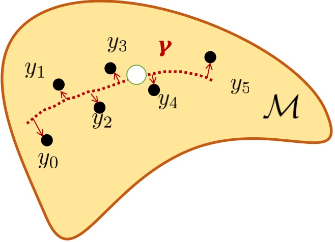
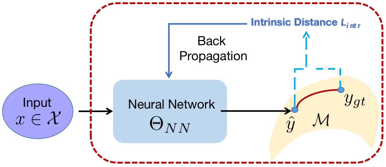
The paper is centered on the third category, which entails creating multiple representations from DNNs. It’s worth noting that models that produce outputs on the manifold are typically regularized using geometric metrics, which can be categorized into two types: intrinsic manifold loss and extrinsic manifold loss (Bhattacharya & Patrangenaru, 2003; Bhattacharya et al., 2012), as depicted in Figure 1. Intrinsic methods aim to identify the geodesic that best fits the data to preserve the geometrical structure (Fletcher, 2011, 2013; Cornea et al., 2017; Shin & Oh, 2022). However, the inherent characteristics of intrinsic distances pose challenges for DNN architectures. Primarily, many intrinsic losses incorporate intricate geodesic distances, aiming to induce longer gradient flows throughout the entire computation graph (Fletcher, 2011; Hinkle et al., 2012; Fletcher, 2013; Shi et al., 2009; Berkels et al., 2013; Fletcher, 2011). Secondly, directly fitting a geodesic by minimizing distance and smoothness energy in the Euclidean space might result in off-manifold points (Chen et al., 2021; Khayatkhoei et al., 2018).
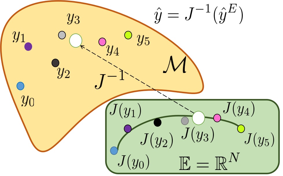
In contrast, extrinsic regression uses embeddings in a higher-dimensional Euclidean space to create a non-parametric proxy estimator. The estimation on the manifold can be achieved using , which represents the inverse of the extrinsic embedding . Extensive investigations in (Bhattacharya et al., 2012; Lin et al., 2017) have established that extrinsic regression offers superior computational benefits compared to intrinsic regression. Many regression models are customized for specific applications, utilizing exclusive information to simplify model formulations that include explicit explanatory variables. This customization is evident in applications such as shapes on shape space manifolds (Berkels et al., 2013; Fletcher, 2011).
However, within the computer vision community, deep neural networks are often faced with a large amount of diverse multimedia data. Traditional manifold regression models struggle to handle this varied modeling task due to limitations in representational power. Some recent works have addressed this challenge, such as (Fang et al., 2023) processing manifold inputs with empirical evidence. This paper presents the idea of embedding manifolds externally at the final regression layer of various neural networks, including ResNet and PointNet. This idea is known as Deep Extrinsic Manifold Representation (DEMR). The process is adapted from two perspectives to bridge the gap between traditional extrinsic manifolds and neural networks in computer vision. Firstly, the conventional choice of a proxy estimator, often represented by kernel functions, is substituted with feature extractors in DNNs. Feature extractors like ResNet or PointNet, renowned for their efficacy in specific tasks, significantly elevate the representational power for feature extraction.
Secondly, to project the neural network output onto the preimage of , we depart from deterministic projection methods employed in traditional extrinsic manifold regression. Instead, we opt for a learnable linear layer commonly found in DNN settings. This learnable projection module aligns seamlessly with most DNN architectures and eliminates the need for the manual design of the projection function , a step typically required in prior extrinsic manifold regression models to match the type of the manifold. These choices not only enhance the model’s representational power compared to traditional regression models but also allow for the preservation of existing neural network architectures.
Contribution
We facilitate the generation of manifold output from standard DNN architectures through extrinsic manifold embedding. In particular, we elucidate the rationale behind pose regression tasks performing more effectively as a specialized instance of DEMR. Additionally, we offer theoretical substantiation regarding the feasibility, asymptotic properties, and generalization ability of DEMR for and the Grassmann manifold. Finally, the efficacy of DEMR is validated through its application to two classic computer vision tasks: relative point cloud transformation estimation on and illumination subspace estimation on the Grassmann manifold.
2 DEMR
2.1 Problem Formulation
Estimation in the embedded space
For distribution on manifold of dimension , the extrinsic embedding , from manifold to Euclidean space , has distribution , which is a closed subset of , where . In extrinsic manifold regression, , a compact projection set , mapping to the closest point on . The extrinsic mean set of is , where is the mean set of . In DEMR, is acquired by the neural networks, and the estimation on is then deterministically computed.
Pipeline design
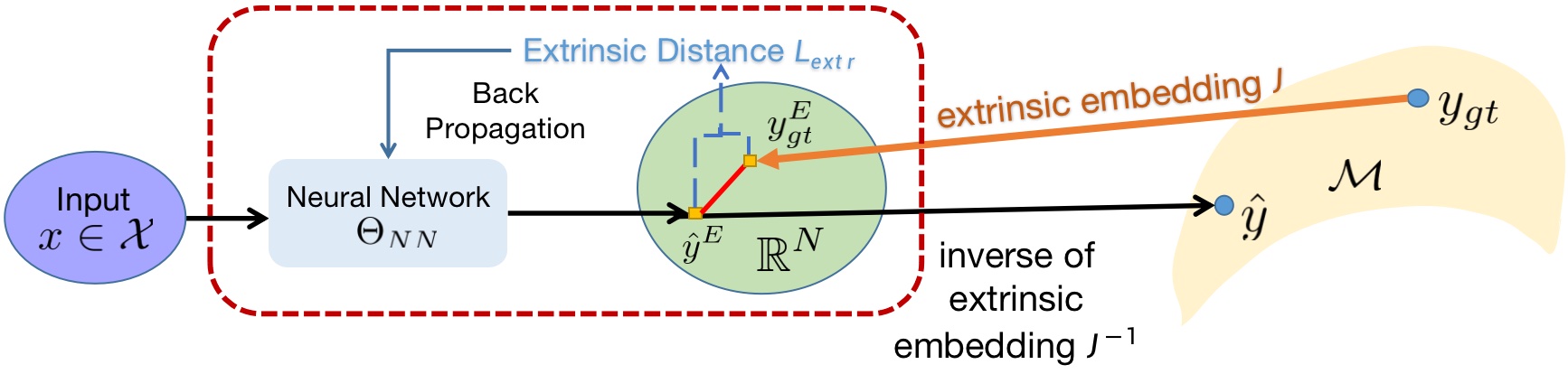
The pipeline of DEMR is demonstrated in Figure 2. For an input with corresponding ground truth estimation , the feedforward process contains two steps; firstly the deep estimation is given in the embedded space , then the output manifold representation is , where is the inverse of extrinsic embedding . Given that , where covers the real-valued vector space of dimension , is then dropped within the pipeline. The training loss is computed between and the extrinsic embedding . Therein, the gradient used in backpropagation is computed within , leaving the original DNN architecture unchanged. Moreover, this implies that the transformation associated with DEMR can be directly applied to most existing DNN architectures by simply augmenting the dimensionality of the final output layer.
Similar to the population regression function in extrinsic regression, the estimator in embedded space as the neural network in extrinsic embedded space aims to minimize the conditional Fréchet mean if it exists: where is the extrinsic distance, denotes the conditional distribution of given , and is the conditional probability measure on . Therefore, in both the training and evaluation phases of DEMR, the computation burden is partaken by the deterministic conversion , which requires no gradient computation.
Reformulation of neural network for images
The input data sample is fed sequentially to the differentiable feature extractor , where the feature extractor can be composited by various modules, such as Resnet, Pointnet, etc., according to the input:
| (1) | ||||
where indicates matrix multiplication, indicates the bias, belongs to the vector matrix of feature maps from , with decomposition into column vectors . Therefore, the DNN in DEMR serves as the composition mapping from raw input to the preimage of .
Projection onto the preimage of
For an extrinsic embedding function , there still exists a pivotal issue that the estimation given above might not lie in the preimage of .
Since , and are all Euclidean and the projection between them can be presented as a linear transform , in matrix forms. Other than a deterministic linear projection in extrinsic manifold regression (Lin et al., 2017; Lee, 2021), DEMR adopts a learnable projection fulfilled by linear layers within a deep framework as in Equation 1, then the output of a DNN is , and . Therefore, the final output of DEMR on the manifold will be
DIMR
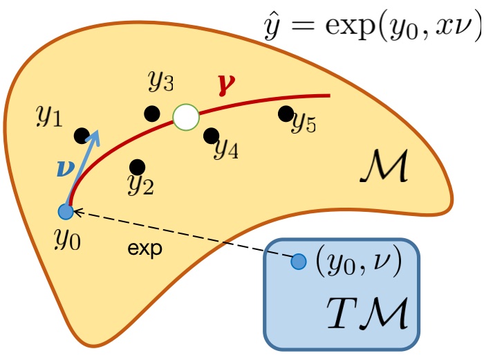
In contrast, the architecture adopted in (Lohit & Turaga, 2017) uses geodesic loss to train the neural network. The intrinsic geodesic distance is in Figure 3, where is the logarithmic map of . We call it Deep Intrinsic Manifold Representation (DIMR) for convenience, whose model parameter set is updated with the gradients of .
2.2 The extrinsic embedding
The embedding is designed to preserve geometric properties to a great extent, which can be specified as equivariance. is considered an equivariant embedding if there is a group homomorphism from to the general linear group of degree such that . There is . Choosing is not unique, and the choices below are equivariant embeddings. Given orthogonal Group Embedding , for with singular value decomposition and and let , then there is and if , there is .
The proof of Grassmannian Embedding follows the same idea with proof for , since they are all based on matrix decomposition.
2.2.1 Matrix Lie Group
9D: SVD of rank 9
An intuitive embedding choice for the matrix Lie group is to parameterize each matrix entry. For the special orthogonal group of dimension , the natural embedding can be given by and . For its inverse, which aims to produce orthogonal vectors, where Gram Schmidt orthogonalization (Zhou et al., 2019) and its variations are common ways to reparameterize orthogonal vectors. Singular Value Decomposition (SVD) is another convenient way to produce an orthogonal matrix (Levinson et al., 2020):
| (2) |
where and come from singular value decomposition with elements arranged according to the descending order of singular value, and is a diagonal matrix with the last entry replaced by . Specifically for , could also be produced by cross product.
As for the special Euclidean group, the group of isometries of the Euclidean space, i.e., the rigid body transformations preserving Euclidean distance. A rigid body transformation can be given by a pair of affine transformation matrix and a translation , or it can be written in a matrix form of size . For instance, a special Euclidean group can be regarded as the semidirect product of a rotation group and a translation group , .
6D: cross product
Specifically for orthogonal matrices on , the invertible embedding can be more convenient via cross-product operation . For a 6-dimensional Euclidean vector as network output, where is the concatenation of and , let , then .
2.2.2 The Quotient Manifold of Lie Group
The real Grassmann manifold parameterize all -dimensional linear subspaces of , which can also be defined by a quotient manifold: . Since it is a quotient space, and we care more about its rank than which basis to provide, we could convert the problem of embedding to finding mappings for , whose basis could be given by diagonal decomposition, which we referred to as . Actually, is a special case of for a symmetric matrix. Thus, for a distribution defined on , given and its diagonal decomposition (denoted by ) , the inverse embedding comes from , and the first column vectors of constitute the subspace.
2.3 DEMR as a generalization of previous research
DNN with Euclidean output
When the output space is a vector space, becomes an identity mapping. Thus, DNN with Euclidean output can be treated as a degenerate form of DEMR. The output from is linearly transformed from the subspace spanned by the base , causing its failure for new extracted features . It is the corresponding failure case in (Zhou et al., 2019), when the dimension of the last layer equals the output dimension.
Absolute/relative pose regression
From Equations 1, the estimation is linearly-transformed from the subspace spanned by . Hence, in typical DNN-based pose regression tasks, the predicted pose can be seen as a linear combination of feature maps extracted from input poses, resulting in the failure of extrapolation for unseen poses in the test set. It is a common problem because training samples are often given from limited poses. (Zhou et al., 2019) suggests that it is the discontinuity in the output space incurs poor generalization. Indeed, a better assumption for APR is that the pose estimation lies on , which is composed of a rotation and a translation. The manifold assumption renders the estimator more powerful in continuous interpolation and extrapolation from input poses. This is because the continuity and symmetry to help a lot in the deep learning task. The detailed analysis is in Section 2.2.1 and validation in Section 4.1 Thereon APR on can be regarded as a particular case solved by DEMR; and (Sattler et al., 2019; Zhou et al., 2019) revealed parts of the idea from DEMR.
3 Analysis
In line with the experimental setup, the analysis is performed on the special orthogonal group, its quotient space, and the special Euclidean group 111All the proofs are included in the Appendix.
3.1 Feasibility of DEMR
Before conducting optimization in extrinsic embedding space , the primary misgiving consists of whether the geometry in extrinsic embedded space properly reflects the intrinsic geometry of .
Apparently, extrinsic embedding is a diffeomorphism preserving geometrical continuity, which is advantageous for extrinsic embeddings. Since we want to observe conformance between and , it’s natural to bridge distances with smoothness. Firstly, we need the diffeomorphism between manifolds to be bilipshitz.
Lemma 3.1.
Suppose that are smooth and compact Riemannian manifolds, is a diffeomorphism. Then is bilipschitz w.r.t. the Riemannian distance.
Then we show in 3.2 the conformity of extrinsic distance and intrinsic distance, which enables indirectly representing an intrinsic loss in Euclidean spaces.
Proposition 3.2.
For a smooth embedding , where the n-manifold is compact, and its metric is denoted by , the metric of is denoted by . For any two sequences of points in and their images , if then .
3.2 Asymptotic MLE
In this part, we demonstrate that DEMR for is the approximate maximum likelihood estimation (MLE) of the response, and for Grassmann manifold DEMR is the MLE of the Grassmann response.
To be noticed, we adopt a new error model in conformity with DEMR. In previous work such as (Levinson et al., 2020), the error noise matrix is assumed to be filled with random entries , which is not rational, because also lies on and there are innate structures between the entries of . Here we assume , so the probability on should be established first.
3.2.1 Lie group for transformations
As (Bourmaud et al., 2015) suggested, we consider the connected, unimodular matrix Lie group, including the most frequently used categories in computer vision: , , , etc. Since is a degenerate case of without translation, here we consider the concentrated Gaussian distribution on . The probability density function (pdf) takes the form , where is the normalizing factor, and the covariance matrix is positive definite.
Maps and are linear isomorphism, re-arranging the Euclidean representations into anti-symmetric matrix and back 222 where indicates the antisymmetric matrix form of the vector. . For a vector , there is and .
Proposition 3.3.
gives an approximation of MLE of rotations on , if assuming , is the identity matrix and an arbitrary real value.
DEMR on special Euclidean Group also approximately provides maximum likelihood estimation, sharing similar ideas of proof with .
Proposition 3.4.
, where the rotation part comes from ((see Supplementary Material) gives an approximation of MLE of transformations on , if assuming , is the identity matrix and an arbitrary real value.
Proof.
Thus, for , there is , and the simplified log-likelihood function is
with set to be , if the pdf focused around the group identity, i.e. the fluctuation of is small, the noise ’s distribution could be approximated by on . Then there is . ∎
3.2.2 Grassmann for subspaces
One of the manifold versions of Gaussian distribution on Grassmann and Stiefel manifolds is Matrix Angular Central Gaussian (MACG). However, the matrix representation of linear subspaces shall preserve the consistency of eigenvalues across permutations and sign flips, thus we resort to the symmetric on Symmetric Positive Definite (SPD) manifold for .
Similarly, the manifold output on the error model is modified to be , where both and are semi-positive definite matrix lying on SPD manifold. The Gaussian distribution extended on SPD manifold, for a random order tensor is
| (3) |
with mean and order covariance tensor inheriting symmetries from three dimensions. For the inverse of Grassmann manifold extrinsic embedding , DEMR provides MLE, and the proofs are given in the Supplementary Material.
Proposition 3.5.
DEMR with gives MLE of element on , if assuming is an identity matrix.
3.3 Generalization Ability
3.3.1 Failure of DNN with Euclidean output space
In light of the analysis in 2.3, the output space is produced by a linear transformation on the convolutional feature space spanned by the extracted features. The feature map extracted by a neural network organized as matrices in Equation (1) the source to form the basis. Denoting the linear subspace spanned by the feature map basis to be and let be the low-dimensional output space spanned by , where denotes the output dimension, then . For a new test input , its extracted feature map belongs to the complementary space of , there is . This accounts for the failure of some DNN models with Euclidean output.
3.3.2 Representation power of structured output space
This section studies the enhancement of the representational power of DEMR, when the output space is endowed with geometrical structure. As a linear action, one representation of a Lie group is a smooth group homomorphism on the -dimensional vector space , where is a general linear group of all invertible linear transformations.
Proposition 3.6.
Any element of dimension on belongs to the image of from known rotations within a certain range, if the Euclidean input of is of more than dimensions.
Corollary 3.7.
Any element of dimension on belongs to the image of from known rotations within a certain range, if the Euclidean input of is of more than dimensions.
Then for a linear representation of Lie group in matrix form, given a set of basis on , we show that the output of DEMR better extrapolates the input samples than common deep learning settings with unstructured output, which resolves the problem raised in (Sattler et al., 2019).
4 Experiments
In this section, we demonstrate the effectiveness of applying extrinsic embedding to deep learning settings on two representative manifolds in computer vision. The experiments are conducted from several aspects below:
-
•
Whether DEMR takes effects in improving the performance of certain tasks?
-
•
Whether the geometrical structure boosts model performance facing unseen cases, e.g., the ability to extrapolate training set.
-
•
Whether extrinsic embedding yields valid geometrical restrictions.
The validations are conducted on two canonical manifold applications in computer vision
4.1 Task I: affine motions on
Estimating the relative position and rotation between two point clouds has a wide range of downstream applications. The reference and target point clouds are in the same size and shape, with no scale transformations. The relative translation and rotation can be arranged separately in vectors or together in a matrix lying on .
4.1.1 Experimental Setup
Training Detail
During training, at each iteration stage, a randomly chosen point cloud from airplanes is transformed by randomly sampling rotations and translations in batches. The rotations are sampled according to the models, i.e., the models producing axis angles are fed with rotations sampled from axis angles, and so on.
Comparison metrics
To validate the ability of the model to preserve geometrical structures, geodesic distance is the opted metric at the testing stage. (Zhou et al., 2019; Levinson et al., 2020) uses minimal angular difference to evaluate the differences between rotations, which is not entirely compatible with Euclidean groups, since it calculates the translation part and rotation part separately. For two rotations and with its trace to be , there is . For intrinsic metric, the geodesic distance between two group elements are defined with Frobenius norm for matrices , where indicates the logarithm map on the Lie group. For extrinsic metric, we take Mean Squared Loss (MSE) between and .
| Mode | avg | median | std |
|---|---|---|---|
| euler | 26.83 | 15.54 | 32.23 |
| axis | 31.96 | 10.66 | 27.75 |
| 6D | 10.28 | 5.36 | 21.54 |
| 9D | 10.23 | 6.09 | 25.30 |
For models with Euler angle and axis-angle output, the predicted rotation and translation are organized in Euclidean form, and they are reorganized into Lie algebra . Finally, the distances are calculated in by exerting an exponential map on their forms.
Architecture detail
Similar as (Zhou et al., 2019; Levinson et al., 2020), the backbone for point cloud feature extraction is composed of a weight-sharing Siamese architecture containing two simplified PointNet Structures (Qi et al., 2017) where . After extracting the feature of each point with an MLP, both and utilize max pooling to produce a single vector respectively, as representations of features across all points in . Concatenating to be , another MLP is used for mapping the concatenated feature to the final higher-order Euclidean representation . Finally, Euler angle quaternion coefficients and axis-angle representations will be directly obtained from the last linear layer of the backbone network of dimension, respectively. For manifold output, the representation will be given by both cross-product and SVD, with details in Supplementary materials. The translation part is produced by another line of layer of 3 dimensions. Because MSE computation between two isometric matrices are based on each entry, total MSE loss is the sum of rotation loss and translation loss.
Estimation accuracy and conformance
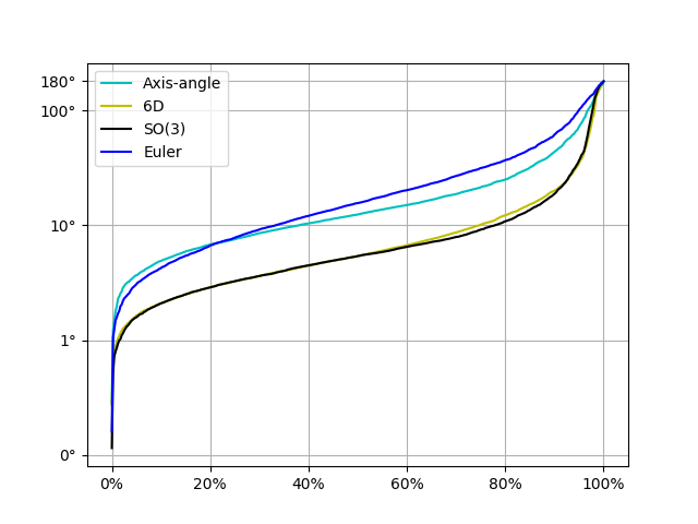
To validate the necessity of structured output space, firstly we compare the affine transformation estimating network with different output formations. The translation part naturally takes the form of a vector and the rotation part can be in the form of Euclidean representations and in matrix forms. The dataset is composed of generated point cloud pairs with random transformations, where the rotations are uniformly sampled from various representations, namely, Euler angle, axis-angle in -dimensional vector space, and . The translation part is randomly sampled from a standard normal distribution.
The advantage of manifold output produced by baseline DEMR is revealed in Table 1 and Figure 4, output via extrinsic embedding takes the lead across three statistics.
| 10% | 20% | 40% | 60% | 80% | |||||||||||
|---|---|---|---|---|---|---|---|---|---|---|---|---|---|---|---|
| avg | med | std | avg | med | std | avg | med | std | avg | med | std | avg | med | std | |
| euler | 77.81 | 54.42 | 77.52 | 35.58 | 13.07 | 48.94 | 28.82 | 17.02 | 30.89 | 27.22 | 16.27 | 35.52 | 27.22 | 16.27 | 31.75 |
| axis | 75.57 | 50.71 | 78.60 | 36.95 | 12.38 | 54.40 | 20.73 | 12.51 | 27.63 | 21.95 | 12.75 | 27.15 | 18.96 | 10.66 | 24.75 |
| 6D | 71.09 | 29.39 | 80.09 | 17.12 | 5.25 | 40.54 | 10.85 | 5.07 | 19.60 | 9.76 | 4.93 | 19.60 | 10.29 | 5.01 | 21.08 |
| 9D | 70.72 | 30.99 | 63.18 | 19.83 | 5.62 | 39.22 | 12.91 | 6.28 | 22.66 | 12.24 | 6.40 | 24.18 | 10.23 | 5.31 | 22.60 |
| Input | GrassmannNet (Lohit & Turaga, 2017) | DIMR | DEMR |
|---|---|---|---|
![[Uncaptioned image]](https://cdn.awesomepapers.org/papers/7dc0a7c8-9d2f-489a-abf6-a68c5c7cd7a8/B13.jpeg)
|
![[Uncaptioned image]](https://cdn.awesomepapers.org/papers/7dc0a7c8-9d2f-489a-abf6-a68c5c7cd7a8/GrassmannNet.jpeg)
|
![[Uncaptioned image]](https://cdn.awesomepapers.org/papers/7dc0a7c8-9d2f-489a-abf6-a68c5c7cd7a8/DIL_B13.jpeg)
|
![[Uncaptioned image]](https://cdn.awesomepapers.org/papers/7dc0a7c8-9d2f-489a-abf6-a68c5c7cd7a8/DEL_B13.jpeg)
|
| avg | 9.6826 | 3.4551 | 3.4721 |
| epoch | 320 | 680 | 140 |
Generalization ability
To evaluate DEMR over its improvement in generalization ability in comparison with unstructured output space, the training set only contains a small portion of the whole affine transformation space while the test set encompasses affine transformations sampled from the whole rotation space. To be fair in the sampling step across the compared representations, the sampling process is conducted uniformly in the representations spaces respectively. For models with axis-angle and Euler angle output, the input point cloud pair is constructed with rotation representation whose entries sampled from Euclidean ranges. For Euler representations, the lower bounds of the ranges are , and the upper bounds are multiplied by , while the test set is sampled from . The training set with axis-angle representations is also obtained by sampling Euclidean ranges. When constructing a training set on , the uniform sampling process is conducted in the same way with axis-angle sampling, the segments are taken in ratios in the same way with the two aforementioned settings, and then exponential mapping is used to yield random samples on . Facing unseen cases, DEMR has better extrapolation capability compared to plain deep learning settings with unstructured output space. As shown in Table LABEL:tab:_generalization, results from deep extrinsic learning show great competence despite the portion size of the training set.
4.2 Task II: illumination subspace, the Grassmann manifold
Changes in poses, expressions, and illumination conditions are inevitable in real-world applications, but seriously impair the performance of face recognition models. It is universally acknowledged that an image set of a human face under different conditions lies close to a low-dimensional Euclidean subspace. After vectorizing images of each person into one matrix in dataset Yale-B (Georghiades et al., 2001), experiments reveal that the top principal components (PC) generally capture more than of the singular values. As an essential application of DEMR, we take the feature extraction CNN as in Equation LABEL:eq:_combination. in high-dimensional Euclidean space, and obtain the final result by inversely mapping the estimation to the Grassmann manifold.
4.2.1 Experimental Setup
Architectural detail
A similar work sharing the same background comes from (Lohit & Turaga, 2017), which assumes the output of the last layer in the neural network to lie on the matrix manifolds or its tangent space. We take GrassmannNet in the former assumption in (Lohit & Turaga, 2017) as the baseline, where the training loss function is set to be Mean Squared Loss. For all the models to be compared, the ratio of the training set is , and all of the illumination angles are adopted. In addition, the data preparation step also follows (Lohit & Turaga, 2017), and other training details are recorded in supplementary materials. On extended Yale Face Database B, each grayscale image of is firstly resized to as the input of CNN, while for subspace ground truth, they are resized to for convenience of computation.
Dataset processing
The input face image indicates the face under the illumination condition, where for Yale B dataset. If we adopt the top PCs, the output is assumed to be in the form of , and where is a Kronecker delta function. Each PC is rearranged as a vector, thus is of size and we define , and the output of the network is . Most of the intrinsic distances defined on the Grassmannian manifold are based on principal angles (PA), for , with SVD where , PAs of Binet-Cauchy (BC) distance is and PAs of Martin (MA) distance is . For comparison of effectiveness and training advantage, the deep intrinsic learning takes as both the training loss and testing metric, where and indicate the ground truth and the network output respectively.
Estimation accuracy and conformance
The results of illumination subspace estimation are given in Table 3. Measured by the average of geodesic losses, DEMR architecture achieves nearly the same performance as DIMR while drastically reducing training time till convergence. With batch size set to be 10, we record training loss after every 10 epochs and report approximately the epoch at which the training loss converged in the third row in Table 3. Besides, both DIMR and DEMR surpass GrassmannNet in the task of illumination subspace estimation, and DEMR still takes fewer epochs for training than GrassmannNet. In the first row of Table 3, on one of the test samples, the results from GrassmannNet, DIMR, and DEMR are displayed. In addition, the conformance of extrinsic and intrinsic metrics can be referred to as supplementary materials.
5 Conclusion
This paper presents Deep Extrinsic Manifold Representation (DEMR), which incorporates extrinsic embedding into DNNs to circumvent the direct computation of intrinsic information. Experimental results demonstrate that retaining the geometric structure of the manifold enhances overall performance and generalization ability in the original tasks. Furthermore, extrinsic embedding exhibits superior computational advantages over intrinsic methods. Looking ahead, the prospect of a more unified formulation for extrinsic embedding techniques within deep learning settings, characterized by parameterized approaches, is envisioned.
References
- Berkels et al. (2013) Berkels, B., Fletcher, P. T., Heeren, B., Rumpf, M., and Wirth, B. Discrete geodesic regression in shape space. In International Workshop on Energy Minimization Methods in Computer Vision and Pattern Recognition, pp. 108–122. Springer, 2013.
- Bermudez et al. (2018) Bermudez, C., Plassard, A. J., Davis, L. T., Newton, A. T., Resnick, S. M., and Landman, B. A. Learning implicit brain mri manifolds with deep learning. In Medical Imaging 2018: Image Processing, volume 10574, pp. 105741L. International Society for Optics and Photonics, 2018.
- Bhattacharya & Patrangenaru (2003) Bhattacharya, R. and Patrangenaru, V. Large sample theory of intrinsic and extrinsic sample means on manifolds. The Annals of Statistics, 31(1):1–29, 2003.
- Bhattacharya et al. (2012) Bhattacharya, R. N., Ellingson, L., Liu, X., Patrangenaru, V., and Crane, M. Extrinsic analysis on manifolds is computationally faster than intrinsic analysis with applications to quality control by machine vision. Applied Stochastic Models in Business and Industry, 28(3):222–235, 2012.
- Boumal (2020) Boumal, N. An introduction to optimization on smooth manifolds. Available online, May, 3, 2020.
- Bourmaud et al. (2015) Bourmaud, G., Mégret, R., Arnaudon, M., and Giremus, A. Continuous-discrete extended kalman filter on matrix lie groups using concentrated gaussian distributions. Journal of Mathematical Imaging and Vision, 51:209–228, 2015.
- Bronstein et al. (2017) Bronstein, M. M., Bruna, J., LeCun, Y., Szlam, A., and Vandergheynst, P. Geometric deep learning: going beyond euclidean data. IEEE Signal Processing Magazine, 34(4):18–42, 2017.
- Bronstein et al. (2021) Bronstein, M. M., Bruna, J., Cohen, T., and Veličković, P. Geometric deep learning: Grids, groups, graphs, geodesics, and gauges. arXiv preprint arXiv:2104.13478, 2021.
- Byravan & Fox (2017) Byravan, A. and Fox, D. Se3-nets: Learning rigid body motion using deep neural networks. In 2017 IEEE International Conference on Robotics and Automation (ICRA), pp. 173–180. IEEE, 2017.
- Can et al. (2021) Can, U., Utku, A., Unal, I., and Alatas, B. Deeper in data science: Geometric deep learning. PROCEEDINGS BOOKS, pp. 21, 2021.
- Cao et al. (2020) Cao, W., Yan, Z., He, Z., and He, Z. A comprehensive survey on geometric deep learning. IEEE Access, 8:35929–35949, 2020.
- Chen et al. (2021) Chen, J., Yin, Y., Birdal, T., Chen, B., Guibas, L., and Wang, H. Projective manifold gradient layer for deep rotation regression. arXiv preprint arXiv:2110.11657, 2021.
- Cornea et al. (2017) Cornea, E., Zhu, H., Kim, P., Ibrahim, J. G., and Initiative, A. D. N. Regression models on riemannian symmetric spaces. Journal of the Royal Statistical Society: Series B (Statistical Methodology), 79(2):463–482, 2017.
- Fang et al. (2023) Fang, Y., Ohn, I., Gupta, V., and Lin, L. Intrinsic and extrinsic deep learning on manifolds. arXiv preprint arXiv:2302.08606, 2023.
- Fletcher (2013) Fletcher, P. T. Geodesic regression and the theory of least squares on riemannian manifolds. International journal of computer vision, 105(2):171–185, 2013.
- Fletcher (2011) Fletcher, T. Geodesic regression on riemannian manifolds. In Proceedings of the Third International Workshop on Mathematical Foundations of Computational Anatomy-Geometrical and Statistical Methods for Modelling Biological Shape Variability, pp. 75–86, 2011.
- Georghiades et al. (2001) Georghiades, A., Belhumeur, P., and Kriegman, D. From few to many: Illumination cone models for face recognition under variable lighting and pose. IEEE Trans. Pattern Anal. Mach. Intelligence, 23(6):643–660, 2001.
- Hinkle et al. (2012) Hinkle, J., Muralidharan, P., Fletcher, P. T., and Joshi, S. Polynomial regression on riemannian manifolds. In European conference on computer vision, pp. 1–14. Springer, 2012.
- Huang et al. (2021) Huang, Z., Cai, H., Dan, T., Lin, Y., Laurienti, P., and Wu, G. Detecting brain state changes by geometric deep learning of functional dynamics on riemannian manifold. In International Conference on Medical Image Computing and Computer-Assisted Intervention, pp. 543–552. Springer, 2021.
- Khayatkhoei et al. (2018) Khayatkhoei, M., Singh, M. K., and Elgammal, A. Disconnected manifold learning for generative adversarial networks. Advances in Neural Information Processing Systems, 31, 2018.
- Lee (2021) Lee, H. Robust extrinsic regression analysis for manifold valued data. arXiv preprint arXiv:2101.11872, 2021.
- Levinson et al. (2020) Levinson, J., Esteves, C., Chen, K., Snavely, N., Kanazawa, A., Rostamizadeh, A., and Makadia, A. An analysis of svd for deep rotation estimation. arXiv preprint arXiv:2006.14616, 2020.
- Lin et al. (2017) Lin, L., St. Thomas, B., Zhu, H., and Dunson, D. B. Extrinsic local regression on manifold-valued data. Journal of the American Statistical Association, 112(519):1261–1273, 2017.
- Lohit & Turaga (2017) Lohit, S. and Turaga, P. Learning invariant riemannian geometric representations using deep nets. In Proceedings of the IEEE International Conference on Computer Vision Workshops, pp. 1329–1338, 2017.
- Ni et al. (2021) Ni, Y., Koniusz, P., Hartley, R., and Nock, R. Manifold learning benefits gans. arXiv preprint arXiv:2112.12618, 2021.
- Qi et al. (2017) Qi, C. R., Su, H., Mo, K., and Guibas, L. J. Pointnet: Deep learning on point sets for 3d classification and segmentation. In Proceedings of the IEEE conference on computer vision and pattern recognition, pp. 652–660, 2017.
- Sattler et al. (2019) Sattler, T., Zhou, Q., Pollefeys, M., and Leal-Taixe, L. Understanding the limitations of cnn-based absolute camera pose regression. In Proceedings of the IEEE/CVF Conference on Computer Vision and Pattern Recognition, pp. 3302–3312, 2019.
- Shi et al. (2009) Shi, X., Styner, M., Lieberman, J., Ibrahim, J. G., Lin, W., and Zhu, H. Intrinsic regression models for manifold-valued data. In International Conference on Medical Image Computing and Computer-Assisted Intervention, pp. 192–199. Springer, 2009.
- Shin & Oh (2022) Shin, H.-Y. and Oh, H.-S. Robust geodesic regression. International Journal of Computer Vision, pp. 1–26, 2022.
- Steinke et al. (2010) Steinke, F., Hein, M., and Schölkopf, B. Nonparametric regression between general riemannian manifolds. SIAM Journal on Imaging Sciences, 3(3):527–563, 2010.
- Yang et al. (2022) Yang, C.-H., Vemuri, B. C., et al. Nested grassmannians for dimensionality reduction with applications. Machine Learning for Biomedical Imaging, 1(IPMI 2021 special issue):1–10, 2022.
- Zhang (2020) Zhang, Y. Bayesian geodesic regression on riemannian manifolds. arXiv preprint arXiv:2009.05108, 2020.
- Zhou et al. (2019) Zhou, Y., Barnes, C., Lu, J., Yang, J., and Li, H. On the continuity of rotation representations in neural networks. In Proceedings of the IEEE/CVF Conference on Computer Vision and Pattern Recognition, pp. 5745–5753, 2019.
Appendix
5.0.1 Proofs in Section 3
Consistency of extrinsic loss and intrinsic loss
Proof of lemma 3.1
Lemma 5.1.
Suppose that are smooth and compact Riemannian manifolds, is a diffeomorphism. Then is bilipschitz w.r.t. the Riemannian distance.
Proof.
For and with smooth metrics and respectively, considering the smooth and continuous map , where indicates the unit tangent bundle of and represents the tangent space, then the function is continuous too. Since is compact, there exists the maximum . Denoting the length of path to be , then there is thus , then is Lipshitz and is Lipshitz. ∎
Proof of proposition 3.2
The extrinsic metric could reflect the tendency of the intrinsic metric. Here we pay more attention to consistency when the losses are small because consistency is crucial in extrinsic loss convergence. To be more specific, for a smooth embedding , where the n-manifold is compact, and its metric is denoted by , the metric of is . The minimal change of suggests the minimal change of , which will be a direct result if is bilipshitz. Here the condition of compactness of the embedded space will be relaxed, where is only desired to be locally bilipshitz, while the proof follows the same idea of the lemma above.
Proposition 5.2.
For a smooth embedding , where the n-manifold is compact, and its metric is denoted by , the metric of is denoted by . For any two sequences of points in and their images , if then .
Proof.
Given that every compact submanifold has positive normal injectivity radius, where , there exists a positive constant , such that with to be the normal bundle of in , and the normal exponential map is a diffeomorphism onto its image . Because the exponential map of is a diffeomorphism, is an open neighborhood of , and the inverse of , is smooth. Let the retraction to be as the composition of the projection and , the closure of to be for , then its image under would be a compact submanifold with boundary . Hence there exists a real constant such that is -Lipshitz on . From lemma 1 there exists a real constant such that is -lipshitz. Moreover, since is the right inverse of the inclusion map , it follows that is -bilipshitz, when restricted to the sufficiently small ball , where .
Next, define the map , where and , and is continuous since the Euclidean distance function and is continuous. For a compact subset , there is a real value such that on is bounded by . Finally, J is locally -bilipshitz, where . Further, for any two sequences of points in and their images , if , there is , . ∎
5.0.2 Asymptotic maximum likelihood estimation (MLE)
Proof of proposition 3.3
Proposition 5.3.
gives an approximation of MLE of rotations on , if assuming , is the identity matrix and an arbitrary real value.
Proof.
For , there is , and the simplified log-likelihood function is
| (4) |
with set to be , if the pdf focused around the group identity, i.e. the fluctuation of is small, the noise ’s distribution could be approximated by on . Then there is . ∎
Proof of proposition 3.4
Proposition 5.4.
where the rotation part comes from , gives an approximation of MLE of transformations on , if assuming , is the identity matrix and an arbitrary real value.
Proof.
Thus, for , there is , and the simplified log-likelihood function is
| (5) |
with set to be , if the PDF focused around the group identity, i.e. the fluctuation of is small, the noise ’s distribution could be approximated by on . Then there is . ∎
Proof of proposition 3.5
For , the probability density function of MACG is
| (6) | ||||
where and covariance matrix is a symmetric positive-definite.
As clarified in section 2.2.2, we obtain Grassmann matrix by equivalently computing on with the diffeomorphic mapping . The error model is modified to be , where both and are semi-positive definite matrix (SPD) . The Gaussian distribution extended on SPD manifold, for a random order tensor (matrix) is
| (7) |
with mean and order covariance tensor inheriting symmetries from three dimensions. To be more specific, and , thereby there is a vectorized version of Equation 3,
| (8) |
where , indicating the unfolded parameters:
| (9) |
Since each entry of comes from rearranging DNN outputs, which can be assumed to not correlate with the other entries, there is when , otherwise , then the likelihood could be further simplified with being an identity matrix. Then there is the proof of proposition 3.5.
Proposition 5.5.
DEL with gives MLE of element on , if assuming is an identity matrix.
Proof.
The log-likelihood function of PDF in Equation (9) is , where and are vectorized versions of and, respectively. ∎
5.1 Generalization Ability
5.1.1 Proof of poposition 5.6
Proposition 5.6.
Any element of dimension on belongs to the image of from known rotations within a certain range, if the Euclidean input of is of more than dimensions.
Proof.
The image of is a set of orthogonal vectors which could span the -dimensional vector space, or it could be regarded as parameterization of rotations around orthogonal axes, so they can be written as .
For the identity , with constant , its solution , which means that if there are orthogonal basis, any rotation could be represented with transformations on . ∎
5.1.2 Proof of corollary 3.7
Corollary 5.7.
Any element of dimension on belongs to the image of from known rotations within a certain range, if the Euclidean input of is of more than dimensions.