Deep Learning for Line Intensity Mapping Observations: Information Extraction from Noisy Maps
Abstract
Line intensity mapping (LIM) is a promising observational method to probe large-scale fluctuations of line emission from distant galaxies. Data from wide-field LIM observations allow us to study the large-scale structure of the universe as well as galaxy populations and their evolution. A serious problem with LIM is contamination by foreground/background sources and various noise contributions. We develop conditional generative adversarial networks (cGANs) that extract designated signals and information from noisy maps. We train the cGANs using 30,000 mock observation maps with assuming a Gaussian noise matched to the expected noise level of NASA’s SPHEREx mission. The trained cGANs successfully reconstruct emission from galaxies at a target redshift from observed, noisy intensity maps. Intensity peaks with heights greater than are located with 60 % precision. The one-point probability distribution and the power spectrum are accurately recovered even in the noise-dominated regime. However, the overall reconstruction performance depends on the pixel size and on the survey volume assumed for the training data. It is necessary to generate training mock data with a sufficiently large volume in order to reconstruct the intensity power spectrum at large angular scales. The suitably trained cGANs perform robustly against variations of the galaxy line emission model. Our deep-learning approach can be readily applied to observational data with line confusion and with noise.
1 Introduction
The large-scale structure of the universe contains rich information on galaxy formation and on the nature of dark matter and dark energy. Line intensity mapping (LIM) is an emerging observational technique that measures the fluctuations of line emission from galaxies and intergalactic medium. With typically low angular and spectral resolutions, LIM can survey an extremely large volume. Future LIM observations are aimed at detecting emission lines at various wavelengths: Hi 21cm line (e.g., SKA; Koopmans et al., 2015), FIR/submillimeter lines such as [Cii] and CO (e.g., TIME; Crites et al., 2014), and ultraviolet/optical lines such as Ly and (e.g., SPHEREx; Doré et al., 2014).
While LIM has the advantage of being able to detect all contributions including emission from faint, dwarf galaxies, there is a serious contamination problem, the so-called line confusion. Because individual line sources are not resolved in LIM observations, foreground/background contamination cannot be easily removed. So far, only a few practical methods have been proposed to extract designated signals. Statistics-based approaches include cross-correlation analysis with galaxies/emission sources from the same redshift (e.g., Visbal & Loeb, 2010), and one that utilizes the anisotropic power spectrum shape (e.g., Cheng et al., 2016). Cheng et al. (2020) devise a method based on sparsity modeling that successfully reconstructs the positions and the line luminosity functions of point sources from multifrequency data.
Earlier in Moriwaki et al. (2020), we have proposed a deep-learning approach to solve the line confusion problem. We use conditional generative adversarial networks (cGANs), which are known to apply to a broad range of image-to-image translation problems. Our cGANs learn the clustering features of multiple emission sources and are trained to separate signals from different redshifts. It is shown that deep learning offers a promising analysis method of data from LIM observations. However, in practice, various noise sources can cause a serious problem. Faint emission-line signals from distant galaxies are likely overwhelmed by noise even with the typical level of next-generation observations.
In this Letter, we propose to use cGANs to effectively de-noise line intensity maps. We show that suitably trained cGANs successfully reconstruct the emission line signals on a map, and recovers basic statistics of the intensity distribution. All such information extracted from noisy maps can be used for studies on cosmology and galaxy population evolution.
2 Methods
We consider emission from galaxies at and observed at 1.5 . The emission is one of the major target lines of future satellite missions such as SPHEREx (Doré et al., 2014) and CDIM (Cooray et al., 2019). We develop cGANs that extract signals from noisy observational data. We first describe how we generate mock intensity maps that are used for training and test. We then explain the basic architecture of our cGANs. Further technical details can be found in Moriwaki et al. (2020).
2.1 Training and test data
We prepare a large set of training and test data. We use a fast halo population code PINOCCHIO (Monaco et al., 2013) that populates a cosmological volume with dark matter halos in a consistent manner with the underlying linear density field. We generate 300 (1000) independent halo catalogs with a cubic box of Mpc on a side for training (test)111In the rest of this Letter, we adopt CDM cosmology with , , and (Planck Collaboration VI, 2018).. The smallest halo mass is . We then assign luminosities to the individual halos to obtain a three-dimensional emissivity field. The halo mass-to-luminosity relation is derived using the result of a hydrodynamics simulation Illustris-TNG (Nelson et al., 2019). We assume that the line luminosity is given by a function of the star-formation rate of the simulated galaxy as
| (1) |
where we adopt mag, and is a coefficient table computed using the photoionization simulation code Cloudy (Ferland et al., 2017).
We work with two-dimensional images (intensity maps) in order to make the best use of modern image translation methods, although, in principle, it is possible to construct neural networks that read and generate three-dimensional data (e.g., Zhang et al., 2019). We generate two-dimensional intensity maps by projecting the three-dimensional emissivity fields along one direction.
For each realization of the training (test) data, 100 maps (1 map) with an area of are generated by projecting random portions of an emissivity field. A total of 30,000 training data and 1000 test data are generated in this manner. The intensity maps are pixelized with the angular and spectral resolution of SPHEREx listed in Table 1.
Finally, realistic mock observation maps are generated by adding Gaussian noise to the intensity map. We adopt the noise level of ”SPHEREx deep” whose sensitivity per pixel at m is 22 mag, corresponding to . The maps are normalized by before input to the networks.
| Field of view | |
|---|---|
| Angular resolution | |
| Spectral resolutiona | 41.5 |
| Sensitivitya |
2.2 Network architecture
We develop cGANs using the publicly available pix2pix code (Isola et al., 2016). The cGANs consist of two adversarial convolutional networks: a generator and a discriminator. The generator, consisting of 8 convolutional and 8 de-convolutional layers, outputs a map (”reconstructed map”) from an observed map . The discriminator, consisting of 4 convolutional layers, returns a value for the input of or with denoting the map. The value indicates the probability that the input is not but . During the training, the two networks are updated repeatedly in an adversarial way; the generator is updated so that it deceives the discriminator (i.e., should get closer to 1), while the discriminator is updated so that it gets better accuracy (i.e., and get closer to 1 and 0, respectively).
Specifically, the parameters in the generator (discriminator) are updated to decrease (increase) the loss function
| (2) |
where
| (3) | |||||
| (4) |
Note that we include an additional term that is known to ensure better performance by imposing the condition that the values of the corresponding pixels in the true and reconstructed maps should be close (Isola et al., 2016). In each round of training, the loss function is computed with a mini-batch. After some experiments, we set and batch size 4. The networks are trained for 8 epochs. We adopt these parameter values throughout the present study.
3 Results
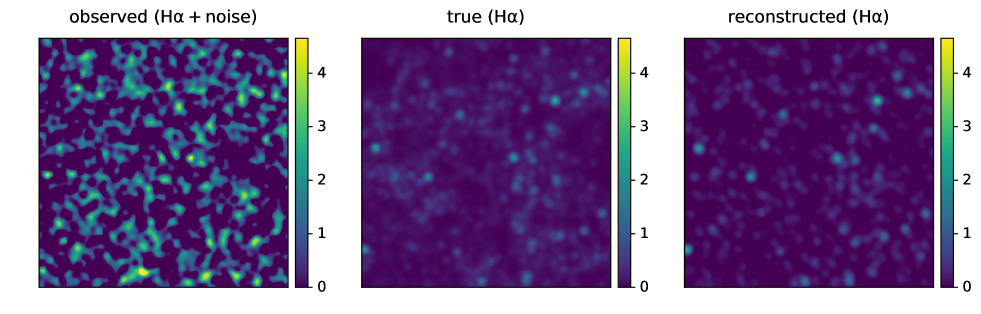
Figure 1 shows the reconstruction performance of our cGANs. Our networks reduce the noise and successfully extract the true signals. It is remarkable that both the source positions and the intensities are reproduced well, even though the observed map is noise dominated. A simpler approach in such a noise-dominated case would be to select only high signal sources in an observed map. However, we find that, if we select pixels with signals greater than from the observed maps, only 20 % of them are true sources (see also Figure 2). With our networks, about 60 % of the reconstructed pixels with intensities greater than are real sources. Hence our method significantly outperforms the simple signal selection based on the local intensity.
3.1 Probability distribution function
The probability distribution function (PDF) of line intensity is an excellent statistic that can constrain galaxy populations and their physical properties (e.g., Breysse et al., 2017). We test whether our networks also recover the PDF accurately.
We first note that, in general, a single set of networks do not reproduce pixel statistics of images/maps robustly. We thus resort to training multiple networks and take the mean of the statistics reconstructed by the ensemble of networks. This technique, called ”bagging,” is known to reduce generalization errors (Goodfellow et al., 2016), and has been applied to, for instance, de-noising weak lensing convergence maps (Shirasaki et al., 2019). In practice, we average the PDFs reconstructed by 5 networks that are trained with different datasets.
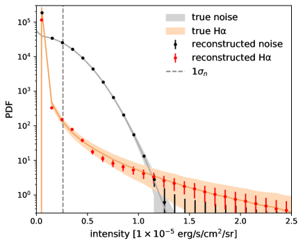
Figure 2 compares the PDFs of true and reconstructed maps. The vertical dashed line indicates the noise level. Our cGANs are able to reconstruct the PDF of the intensity above 1. Note also that the scatter of the averaged PDF lies within the intrinsic scatter of the true maps, i.e., within the so-called cosmic variance. Apparently, the networks tend to reconstruct the PDFs close to the average. This is simply caused by the bagging procedure. We have checked and confirmed that the variance of reconstructed PDFs by a single network is as large as the intrinsic one.
3.2 Power spectrum
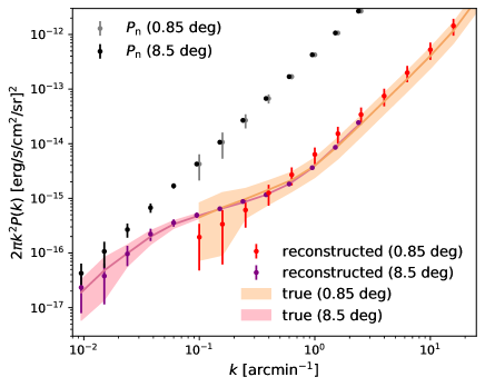
We further examine the ability of our cGANs to reconstruct the intensity power spectrum. To this end, we again adopt the bagging of 5 networks that are trained with different datasets. The red points with error bars and the shaded regions in Figure 3 show the power spectra of the reconstructed and true maps, respectively. We also show the noise power spectrum, , and its variance, , where is the number of modes in . We adopt .
We notice that the reconstructed power spectra on large scales () are systematically underestimated. This might be owing to the finite box size of the training data. To examine this, we train the cGANs with mock intensity maps with a larger area. For this test, we generate halo catalogs in a cubic volume of Mpc on a side (see Section 2.1). Then the smallest halos populated is degraded to , but we have confirmed that the mean intensity (or the total luminosity density) is not significantly different from that with our default box size of Mpc. We set the side length of the pixel and the spectral resolution . Each map has a ten times larger area of . The noise level scales with the angular and spectral resolution as
| (5) |
where , , and are the original angular and spectral resolution and the noise level of SPHEREx (Table 1). The resulting noise level of the wide maps is . We adopt the same hyperparameters in the cGANs as in our default case except we set and the normalization factor for the low-resolution maps. The purple dots with error bars in Figure 3 show the power spectrum of the reconstructed wide maps. The light-pink shading indicates the 1 dispersion of the true power spectra. Clearly, the large-scale (low-) power spectrum is reconstructed more accurately compared to our default case. We note that the cGANs trained with the wider maps do not resolve point sources, but the peaks and voids in the reconstructed map correspond closely to the positions of groups/clusters and void regions.
Ideally, networks trained with intensity maps that have fine pixels and a large box size would be able to reconstruct both the positions of point sources (galaxies) and their large-scale clustering. Unfortunately, it becomes computationally more expensive if we set a larger number of pixels. The computational time for training roughly scales with the number of pixels, and the necessary number of training epochs could also increase. We thus suggest that one should generate training data depending on the purpose. In order to detect point sources robustly, one needs to train the networks using fine-pixel maps. If the primary purpose is to reconstruct the large-scale power spectrum, for cosmology studies for instance, then one needs to generate maps with a sufficiently large area (volume) but with coarse pixels. The reconstructed power spectra shown in Figure 3 suggest that one should adopt at least a several times larger area for training than the actual size of observed maps.
3.3 Line emission models
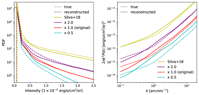
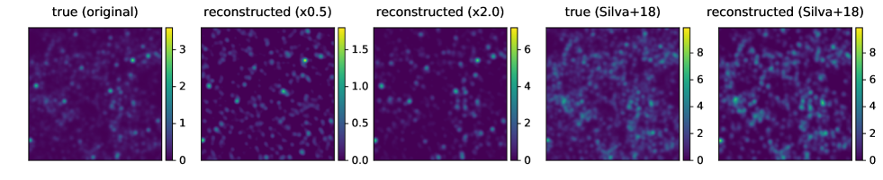
The line intensities of high-redshift galaxies are not well constrained observationally, and theoretical models of galaxy formation and evolution remain uncertain. Thus it is important to examine whether our GAN-based method can be applied robustly to data that are generated with different line emission models. To this end, we generate three additional sets of 1000 test data that have the same noise level but have different line intensities. Two of the new test datasets are generated by simply multiplying the original maps by a constant value, and 2, as
| (6) |
These cases serve as a test of the networks’ reconstruction performance against the variation in the mean intensity. We also adopt a completely different model of emission, Silva et al. (2018), in which the SFR-halo mass relation derived by Guo et al. (2013) is used to assign the luminosities ( SFR). The model reproduces the mean intensity consistent with observations (Sobral et al., 2013, 2015).
Figure 4 shows examples of reconstructed images. In all the cases, the locations and amplitudes of bright peaks are reconstructed well, even though the mean intensity levels are quite different from the original data (see the color bars). It appears that the networks practically learn the noise properties and extract the signal robustly, even if the signal amplitude is different from the training data. It is remarkable that, in the cases with and with Silva et al. (2018) model, the signals are reconstructed as accurately as the default case.
We also compare the one-point PDFs and the power spectra in Figure 5, where we plot the averages over 1000 test data with (cyan line), 1 (red), and 2 (purple), respectively. The yellow lines show those with the Silva et al. (2018) model. The statistics of each reconstructed image are computed by taking the means of those reconstructed by 5 different networks. Both the one-point PDFs and the power spectra are reproduced well except the case of that has effectively small signals. We thus conclude that our network is applicable to maps with different intensity models as long as we have a good understanding of the observational noise and if the line intensities are not too weak compared to the training data.
4 Conclusion
We have developed cGANs that effectively reduce observational noise in line intensity maps. We train the cGANs by using a large set of mock observations assuming a realistic noise level expected for the SPHEREx mission. Our cGANs can reconstruct the point-source positions and the PDF of the intensity maps. The power spectrum is also reconstructed remarkably well, but the accuracy depends on the area/volume assumed for the training data. We have also found that our method is able to reconstruct the signals even if the underlying line intensity model is different from the original training data.
If we combine with another set of networks that efficiently separates signals from different redshifts (Moriwaki et al., 2020), the cGANs developed in this study can extract the emission-line signal from galaxies at an arbitrarily specified redshift from noisy maps. Therefore, using data from multi-frequency, wide-field intensity mapping observations, we can reconstruct the three-dimensional distribution of emission-line galaxies. The intensity peaks detected by our cGANs correspond to bright galaxies and galaxy groups with high confidence, which will be promising targets for follow-up observations. Finally, the reconstructed line intensity map essentially traces the distribution of galaxies and hence of underlying matter, and thus it is well suited for cross-correlation analysis with other tracers. Accurate reconstruction of the statistics such as the one-point PDF and power spectrum as shown in this Letter will allow us to perform cosmological parameter inference and to study galaxy formation and evolution using data from future LIM observations.
References
- Breysse et al. (2017) Breysse, P. C., Kovetz, E. D., Behroozi, P. S., Dai, L., & Kamionkowski, M. 2017, MNRAS, 467, 2996, doi: 10.1093/mnras/stx203
- Cheng et al. (2016) Cheng, Y.-T., Chang, T.-C., Bock, J., Bradford, C. M., & Cooray, A. 2016, ApJ, 832, 165, doi: 10.3847/0004-637X/832/2/165
- Cheng et al. (2020) Cheng, Y.-T., Chang, T.-C., & Bock, J. J. 2020, ApJ, 901, 142, doi: 10.3847/1538-4357/abb023
- Cooray et al. (2019) Cooray, A., Chang, T.-C., Unwin, S., et al. 2019, arXiv e-prints, arXiv:1903.03144. https://arxiv.org/abs/1903.03144
- Crites et al. (2014) Crites, A. T., Bock, J. J., Bradford, C. M., et al. 2014, Proc. SPIE, 9153, 91531W, doi: 10.1117/12.2057207
- Doré et al. (2014) Doré, O., Bock, J., Ashby, M., et al. 2014, arXiv e-prints, arXiv:1412.4872. https://arxiv.org/abs/1412.4872
- Ferland et al. (2013) Ferland, G. J., Porter, R. L., van Hoof, P. A. M., et al. 2013, Rev. Mexicana Astron. Astrofis., 49, 137. https://arxiv.org/abs/1302.4485
- Ferland et al. (2017) Ferland, G. J., Chatzikos, M., Guzmán, F., et al. 2017, Rev. Mexicana Astron. Astrofis., 53, 385. https://arxiv.org/abs/1705.10877
- Goodfellow et al. (2016) Goodfellow, I., Bengio, Y., & Courville, A. 2016, Deep Learning (MIT Press)
- Guo et al. (2013) Guo, Q., White, S., Angulo, R. E., et al. 2013, MNRAS, 428, 1351, doi: 10.1093/mnras/sts115
- Isola et al. (2016) Isola, P., Zhu, J., Zhou, T., & Efros, A. A. 2016, CoRR, abs/1611.07004. https://arxiv.org/abs/1611.07004
- Koopmans et al. (2015) Koopmans, L., Pritchard, J., Mellema, G., et al. 2015, in Advancing Astrophysics with the Square Kilometre Array (AASKA14), 1. https://arxiv.org/abs/1505.07568
- Monaco et al. (2013) Monaco, P., Sefusatti, E., Borgani, S., et al. 2013, MNRAS, 433, 2389, doi: 10.1093/mnras/stt907
- Moriwaki et al. (2020) Moriwaki, K., Filippova, N., Shirasaki, M., & Yoshida, N. 2020, MNRAS, 496, L54, doi: 10.1093/mnrasl/slaa088
- Nelson et al. (2019) Nelson, D., Springel, V., Pillepich, A., et al. 2019, Computational Astrophysics and Cosmology, 6, 2, doi: 10.1186/s40668-019-0028-x
- Planck Collaboration VI (2018) Planck Collaboration VI. 2018, arXiv e-prints, arXiv:1807.06209. https://arxiv.org/abs/1807.06209
- Shirasaki et al. (2019) Shirasaki, M., Yoshida, N., & Ikeda, S. 2019, Phys. Rev. D, 100, 043527, doi: 10.1103/PhysRevD.100.043527
- Silva et al. (2018) Silva, B. M., Zaroubi, S., Kooistra, R., & Cooray, A. 2018, MNRAS, 475, 1587, doi: 10.1093/mnras/stx3265
- Sobral et al. (2013) Sobral, D., Smail, I., Best, P. N., et al. 2013, MNRAS, 428, 1128, doi: 10.1093/mnras/sts096
- Sobral et al. (2015) Sobral, D., Matthee, J., Best, P. N., et al. 2015, MNRAS, 451, 2303, doi: 10.1093/mnras/stv1076
- Visbal & Loeb (2010) Visbal, E., & Loeb, A. 2010, J. Cosmology Astropart. Phys, 11, 016, doi: 10.1088/1475-7516/2010/11/016
- Zhang et al. (2019) Zhang, X., Wang, Y., Zhang, W., et al. 2019, arXiv e-prints, arXiv:1902.05965. https://arxiv.org/abs/1902.05965