Deep Learning modelling of the Limit Order Book:
a comparative perspective
Abstract
The present work addresses theoretical and practical questions in the domain of Deep Learning for High Frequency Trading. State-of-the-art models such as Random models, Logistic Regressions, LSTMs, LSTMs equipped with an Attention mask, CNN-LSTMs and MLPs are reviewed and compared on the same tasks, feature space, and dataset and clustered according to pairwise similarity and performance metrics. The underlying dimensions of the modelling techniques are hence investigated to understand whether these are intrinsic to the Limit Order Book’s dynamics. We observe that the Multilayer Perceptron performs comparably to or better than state-of-the-art CNN-LSTM architectures indicating that dynamic spatial and temporal dimensions are a good approximation of the LOB’s dynamics, but not necessarily the true underlying dimensions.
Keywords Artificial Intelligence Deep Learning Econophysics Financial Markets Market Microstructure
1 Introduction
Recent years have seen the growth and spreading of Deep Learning methods across several domains. In particular, Deep Learning has been increasingly applied to the domain of Financial Markets. However, these activities are mostly performed in industry and there is a scarce academic literature to date. The present work builds upon the general Deep Learning literature to offer a comparison between models applied to High Frequency markets. Insights about Market Microstructure are then derived from the features and performance of the models.
The Limit Order Book (LOB) represents the venue where buyers and sellers interact in an order-driven market. It summarises a collection of intentions to buy or sell integer multiples of a base unit volume (lot size) at price . The set of available prices is discrete with a basic unit step (tick size). The LOB is a self-organising complex process where a transaction price emerges from the interaction of a multitude of agents in the market. These agents interact through the submission of a range of order types in the market. Figure 1 provides a visual representation of the LOB, its components and features.
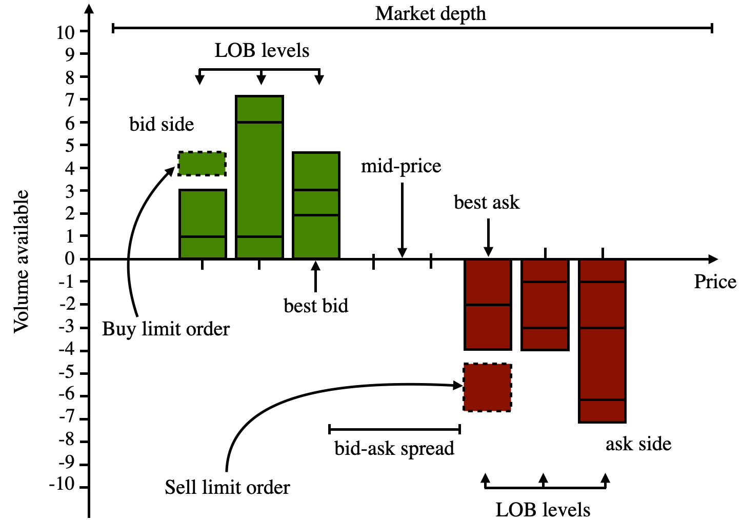
Three main categories of orders exist: market orders, limit orders and cancellation orders. Market orders are executed at arrival by paying a higher execution cost which originates from crossing the bid-ask spread. Limit orders make up the liquidity of the LOB at different price levels and constitute an expression of the intent to buy or sell a given quantity at a specific price . These entail lower transaction costs, with the risk of the order not being fulfilled. Cancellation orders are used to partially or fully remove limit orders which have not been filled yet.
The study of order arrival and dynamics of the Limit Order Book and of order-driven markets has seen a growing interest in the academic literature as well as in the industry. This sparked from the almost simultaneous spreading of electronic trading and high frequency trading (HFT) activity throughout global markets. The resulting increase in frequency of the trading activity has generated a growing amount of trading data thereby creating the critical mass for Big Data applications.
The availability of Big Data from High Frequency Trading has then made it possible to apply the data hungry Machine Learning and Deep Learning methods to financial markets. Machine Learning methods were initially adopted by hedge funds towards the end of the last century, while now adoption is expanding and it is possible to see large quantitative firms and leading investment banks openly applying AI methods. Building upon this growing interest, an increasing number of papers and theses exploring Machine Learning and Deep Learning methods applied mostly to financial markets are being written. This is part of the modern trend where large companies lead research fields in AI due to the availability of computational and monetary resources [17, 30]. This often results in a literature dominated by increasingly complex and task-specific model designs, often conceived adopting an applicative approach without an in-depth analysis of the theoretical implications of obtained results.
In light of this, for the present work, the relevant literature has been screened in search of state-of-the-art models for price movement forecasting in high frequency trading. Increasingly complex models from this literature are presented, characterised and results are compared on the same training and test sets. Theoretical implications of these results are investigated and they are compared for statistically validated similarity. This analysis has the purpose to reason why certain models should or should not be used for this application as well as verify whether more complex architectures are truly necessary. One example of this consists in the performed study of temporal and spatial dimensions (implied by Recurrent Neural Network (RNN) [31], Attention [39] and Convolutional Neural Network (CNN) [29] models, respectively) and whether they are unique and optimal representations of the Limit Order Book. The alternative hypothesis consists in a Multilayer Perceptron (MLP) which does not explicitly model any dynamic.
The Deep Learning models described in Section 2, incorporate assumptions about the structure and relations in the data as well as how it should be interpreted. As reported above, this is the case of CNNs which exploit the relations between neighbouring elements in their grid-like input. Analogous considerations can be made for RNN-like models, which are augmented by edges between consecutive observation embeddings. These types of structures aim to carry information across a series, hence implying sequential relations between inputs. These tailored architectures are used to test hypotheses about the existence and informativeness of corresponding dimensional relations in the Limit Order Book.
The diffusion of flexible and extensible frameworks such as Weka [41] and Keras [10], and the success of automated Machine Learning tools such as AutoML [21] and H2O AutoML [8], is facilitating the abovementioned industry driven applicative approach. Unfortunately, much less attention is given to methods for model comparison able to asses the real improvement brought by these new models [13]. In order to make the work presented here more reliable and to promote a more thorough analysis of published works, a statistical comparison between models is provided through the state-of-the-art statistical approaches described in [4].
It is crucial for scientifically robust results to validate the significance of model performance and the potential performance improvements brought by novel architectures and methodologies. The main classes of methods for significance testing are Frequentist and Bayesian. Null model-based Frequentist methods are not ideal for this application as the detected statistical significance might have no practical impact on performance. The need to answer questions about the likelihood of one model to perform significantly better than another, based on experiments requires the use of posterior probabilities, which can be obtained from the Bayesian methods as, for instance, in [16, 14, 5].
This paper is organised in the following sections: Section 2 presents a review of the relevant literature which motivates the study performed in the current work and presents the assumptions upon which it is built. Section 3 briefly describes the data used throughout the experiments. Section 4 provides an exhaustive description of the experiments conducted. Section 5 presents and analyses the results and Section 7 concludes the work with ideas for further research efforts.
2 Related Work
The review by Bouchaud et al. [6] offers a thorough introduction to Limit Order Books, to which the interested reader is referred. As discussed in Section 1, the growth of electronic trading has sparked the interest in Deep Learning applications to order-driven markets and Limit Order Books. The work by Kearns and Nevmyvaka [26] presents an overview of Machine Learning and Reinforcement Learning applications to market microstructure data and tasks, including return prediction from Limit Order Book states. To our knowledge, the first attempt to produce an extensive analysis of Deep Learning-based methods for stock price prediction based upon the Limit Order Book was made by Tsantekidis et al. [38]. In that paper, starting from a horse racing-type comparison between classical Machine Learning approaches (e.g. Support Vector Machines) and more structured Deep Learning ones, they then considered the possibility to apply CNNs to detect anomalous events in the financial markets, and take profitable positions. In the last two years a few works applying a variety of Deep Learning models to LOB-based return prediction were published by the research group of Stephen Roberts, the first one, to the best of our knowledge, applied Bayesian (Deep Learning) Networks to Limit Order Book [43], followed by an augmentation to the labelling system as quantiles of returns and an adaptation of the modeling technique to this [44]. The most recent work introduces the current state-of-the-art modeling architecture combining CNNs and LSTMs to delve deeper into the complex structure of the Limit Order Book. The work by Sirignano and Cont [37] provides a more theoretical approach, where it tests and compares multiple Deep Learning architectures for return forecasting based on order book data and shows how these models are able to capture and generalise to universal price formation mechanisms throughout assets.
The models used in the above works were originally defined in the literature from the field of Machine and Deep Learning and are summarised hereafter.
Multinomial Logistic Regression is used as a baseline for this work and consists in a linear combination of the inputs mapped through a logit activation function, as defined in [19].
Feedforward Neural Networks (or Multilayer Perceptrons) are defined in [22] and constitute the general framework to represent non-linear function mappings between a set of input variables and a set of output variables. Recurrent Neural Networks (RNNs) [31] are considered in the form of Long-Short Term Memory models (LSTMs) [23]. RNNs constitute an evolution of MLPs. They introduce the concept of sequentiality into the model including edges which span adjacent time steps. RNNs suffer from the issue of vanishing gradients when carrying on information for a large number of time steps. LSTMs solve this issue by replacing nodes in the hidden layers with self-connected memory cells of unit edge weight which allow to carry on information without vanishing or exploding gradients. LSTMs hence owe their name to the ability to retain information through a long sequence. The addition of Attention mechanisms [39] to MLPs helps the model to focus more on relevant regions of the input data in order to make predictions. Self-Attention extends the parametric flexibility of global Attention Mechanisms by introducing an Attention mask that is no longer fixed, but a function of the input. The last kind of Deep Learning unit considered are Convolutional Neural Networks (CNNs), designed to process data with grid-like topology. These unit serve as feature extractors, thus learning feature representations of their inputs [29].
A considerable body of literature about comparison of different models has been produced, despite not being vastly applied by the Machine Learning community. The first attempts of formalisation were made by Ditterich [15] and Salzberg [35], and refined by Nadau and Bengio [33] and Alpaydm [2]. A comprehensive review of all these methods and of classical statistical tests for Machine Learning is presented in [25]. A crucial point of view is provided by the work [13]. More recently, starting from the work by Corani and Benavoli [12], a Bayesian approach to statistical testing was proposed to replace classical approaches based on the null hypothesis. The proposed new ideas found a complete definition in [4].
3 Dataset
All the experiments presented in this paper are based on the usage of the LOBSTER [24] dataset, which provides a highly detailed, event-by-event description of all micro-scale market activities for each stock listed on the NASDAQ exchange. LOBSTER is one of the data providers featured in some major publications and journals in this field. LOB datasets are provided for each security in the NASDAQ. The dataset lists every market order arrival, limit order arrival and cancellation that occurs in the NASDAQ platform between 09:30 am – 04:00 pm on each trading day. Trading does not occur on weekends or public holidays, so these days are excluded from all the analyses performed. A tick size of is adopted. Depending on the type of the submitted order, orders can be executed at the lower cost equals of . This is the case of hidden orders which, when revealed, appear at a price equal to the notional mid-price at the time of execution.
LOBSTER [24] data are structured into two different files:
-
•
The message file lists every market order arrival, limit order arrival and cancellation that occurs.
-
•
The orderbook file describes the market state (i.e. the total volume of buy or sell orders at each price) immediately after the corresponding event occurs.
Experiments described in the next few sections are performed only using the orderbook files. The training dataset consists of Intel Corporation’s (INTC) LOB data from 04-02-2019 to 31-05-2019, corresponding to a total of 82 files, while the test dataset consists of Intel Corporation’s LOB data from 03-06-2019 to 28-06-2019, obtained from 20 other files.
It is relevant to highlight that INTC is representative of a large tick stock, these are stocks where the tick size is relative large compared to the price. These stocks present a range of specific characteristics in their LOB and trading dynamics and have been observed to be more predictable, through Deep Learning models, than small tick stocks. Hence, most of the market microstructure-related AI literature considers large tick stocks.
All the experiments presented in the current work are conducted on snapshots of the LOB with a depth (number of tick size-separated limit order levels per side of the Order Book) of . This means that each row in the orderbook files corresponds to a vector of length 40. Each row is structured as
| (1) |
where represents the price level and corresponding liquidity tuple, distinguish ask and bid levels progressively further away from the best ask and best bid.
4 Methods
4.1 Price change horizons
Price log-returns for the target labels are defined at three distinct time horizons . In order to account for price volatility and discount long periods of stable and noisy order flow, the time delay between the LOB observation (input) and the target label return is defined as follows.
Given a series of mid-prices at consecutive ticks
| (2) |
the mid-price is defined as the mean between the best bid and best ask price. The series of log-returns is
| (3) |
where
| (4) |
The number of non-zero log-returns in the series is hence counted as:
| (5) |
where is the Heaviside step function defined below
| (6) |
4.2 Data preprocessing and labelling
The data described in Section 3 are preprocessed as follows:
-
•
The target labels for the prediction task aim to categorise the return at three different time horizons . In order to perform the mapping from continuous variables into discrete classes, the following quantile levels are computed on the returns distribution of the training set and then applied to the test set. These quantiles are mapped onto classes, denoted with as reported in Figure 2.
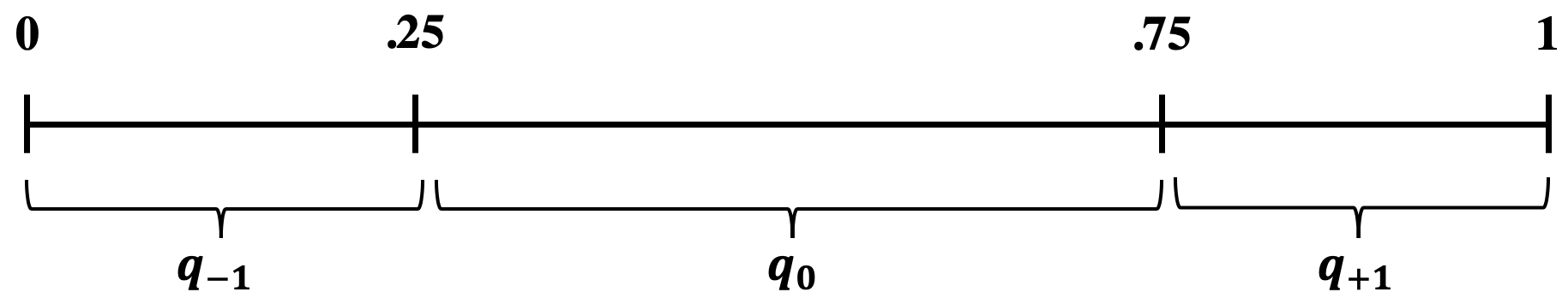
Figure 2: Visual representation of the mapping between quantiles and corresponding classes. Quantiles’ edges (i.e. ) define three different intervals. Each specific class (i.e. , , ) corresponds to a specific interval. -
•
The training set input data (LOB states) are scaled within a interval with the
min-maxscaling algorithm [34]. The scaler’s training phase is conducted by chunks to optimise the computational effort. The trained scaler is then applied to the test data.
Figure 3 reports the training and test set quantile distributions per horizon .
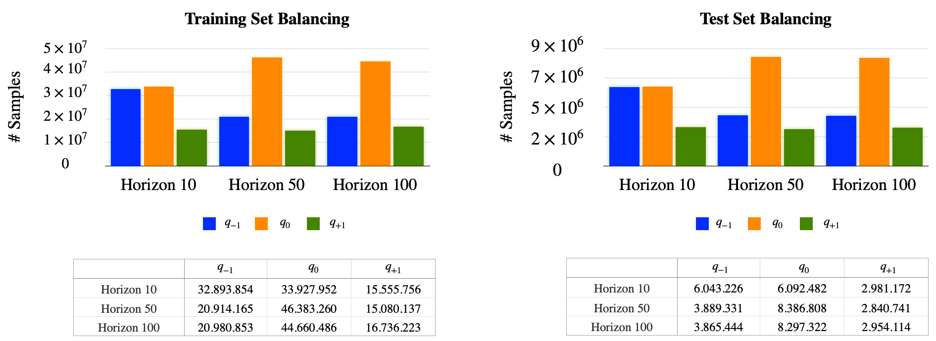
It is possible to notice moderately balanced classes for both plots in Figure 3. Indeed, all classes lie within the same order of magnitude () for all horizons with the class being the most represented and the least.
4.3 Random Model
The benchmark null model for this work is a generic random model, which does not handle any dynamics. For each sample in the test set and each horizon , the quantile label is sampled from the uniform distribution over . The SciPy [40] randint generator is used for this task.
4.4 Naive Model
4.5 Logistic Regression
The baseline model is represented by the multinomial Logistic Regression which, as the Random Model, does not explictly model any dynamics in the data. Like binary Logistic Regression, the multinomial one adopts maximum likelihood estimation to evaluate the probability of categorical membership. It is also known as Softmax Regression and can be interpreted as a classical ANN, as per the definition in Table 1, with the input layer directly connected to the output layer with a softmax activation function:
| (7) |
The input is represented by the ten most recent LOB states as per the definition is Equation 1 in Section 3. Also this model is not able to handle any specific dynamics. The Scikit-Learn [34] implementation is used and, in order to guarantee a fair comparison with the Deep Learning models in the next sections, the following parameters are set as follows:
-
•
max_iter (i.e. maximum number of iterations taken for the solvers to converge) = 20.
-
•
tol (i.e. the tolerance for stopping criteria) = .
-
•
solver (i.e. the algorithm to use in the optimization problem) =
sagwith the default penalty.
Logistic regression
Input @ []
Dense @ 3 Units (activation softmax)
4.6 Multilayer Perceptron
The first Deep Learning model is a generic Multilayer Perceptron (MLP), which does not explicitly model temporal or spatial properties of the input data, but has the ability to model not explicitly defined dimensions through its hidden layers. Similarly to the two previously mentioned models, it does not explicitly handle any specific dimension. The MLP can be considered the most general form of universal approximator and it represents the ideal model to confirm or reject any hypothesis about the presence of a specific leading dimension in LOBs.
In order to allow a fair comparison with the other sequence-based models, the input for the MLP is represented by a vector containing the ten most recent LOB states (see Equation 1) concatenated in a flattened shape. The MLP model is architecturally defined in Table 2.
Multilayer Perceptron
Input @ []
Dense @ 512 Units
Dense @ 1024 Units
Dense @ 1024 Units
Dense @ 64 Units
Dense @ 3 (activation softmax)
4.7 Shallow LSTM
In order to explicitly handle temporal dynamics of the system, a shallow LSTM model is tested [23]. The LSTM architecture explicitly models temporal and sequential dynamics in the data, hence providing insight on the temporal dimension of the data. As all the other RNN models, the structure of LSTMs enables the network to capture the temporal dynamics performing sequential predictions. The current state directly depends on the previous ones, meaning that the hidden states represent the memory of the network. Differently from classic RNN models, LSTMs are explicitly designed to overcome the vanishing gradient problem as well as capture the effect of long-term dependencies. The input is here represented by a matrix, where 10 is the number of consecutive history ticks and 40 is the shape of the LOB defined in Equation 1. The LSTM layer consists of 20 units with a activation function:
| (8) |
It is observed that the addition of LSTM units beyond the chosen level does not yield statistically significant performance improvements. Hence, the chosen number of LSTM units can be considered optimal and the least computationally costly. The model is architecturally defined in Table 3.
Shallow LSTM
Input @ []
LSTM @ 20 Units
Dense @ 3 Units (activation softmax)
4.8 Self-Attention LSTM
As a point of contact between architectures which model temporal dynamics (LSTMs) and spatial modeling ones (CNNs), the LSTM described in Section 4.7 is enhanced by the introduction of a Self-Attention module [39]. By default, the Attention layer statically considers the whole context while computing the relevance of individual entries. Differently from what described in Section 4.9, the input is not subject to any spatial transformation (e.g. convolutions). This difference implies a static nature of the detected behaviours over multiple timescales. The Self-Attention LSTM is architecturally defined in Table 4.
Self-attention LSTM
Input @ []
LSTM @ 40 Units
Self-Attention Module
Dense @ 3 (activation softmax)
The input to this model is represented by a matrix, where 10 is the number of consecutive history ticks and 40 is the shape of the LOB defined in Equation 1.
4.9 CNN-LSTM
The nature of the Deep Learning architectures in Sections 4.7, 4.8 mainly focuses on modeling the temporal dimension of the inputs. Recent developments [42, 36] highlight the potential of the spatial dimension in LOB-based forecasting as a structural module allowing to capture dynamic behaviours over multiple timescales. In order to study the effectiveness of such augmentation, the architecture described in [42, 7] is reproduced as in Table 5, and adapted to the application domain described in the current work. The input is represented by a matrix, where 10 is the number of consecutive history ticks and 40 is the shape of the LOB defined in Equation 1. This model represents the state-of-the-art in terms of prediction potential at the time of writing.
CNN-LSTM
Input @ []
Conv
@ 16 (stride = )
@ 16
@ 16
@ 16 (stride = )
@ 16
@ 16
@ 16
@16
@ 16
Inception @ 32
LSTM @ 64 Units
Dense @ 3 (activation softmax)
4.10 Training pipeline
For each of the Deep Learning models, the following training (and testing, see Section 4.11) procedure is applied:
- •
-
•
For each training epoch batches are randomly chosen. This number of batches is selected to consider a total number of training samples equivalent to one month ( samples). This sampling procedure ensures a good coverage of the entire dataset and allows to operate with a reduced amount of computational resources.
-
•
Class labels are converted to their one-hot representation.
- •
-
•
From manual hyperparameter exploration it is observed that 30 training epochs are optimal when accounting for constraints on computational resources. It has been empirically observed that slight variations do not produce any significant improvement.
4.11 Test pipeline and performance metrics
At the end of the training phase, the inducer for each model is queried on the test set as follows:
- •
-
•
For each model and test fold, balanced Accuracy [32, 27, 20], weighted Precision, weighted Recall and weighted F-score are computed. These metric are weighted in order to correct for class imbalance and obtain unbiased indicators. The following individual class metrics are considered too: Precision, Recall and F-measure. Two multi-class correlation metrics between labels are also computed: Matthews Correlation Coefficient (MCC) [18] and Cohen’s Kappa [11, 3].
-
•
Performance metrics for each test fold are statistically compared through the Bayesian correlated t-test [12, 4]. One should note that the region of practical equivalence (rope) determining the negligible difference between performance metrics in different models, is arbitrarily set to a sensible , due to the lack of examples in the literature.
| Model | Dimension |
|---|---|
| Random Model & Naive Model | None |
| Multinomial Logistic Regression | None |
| Multilayer Perceptron | Not explicitly defined |
| Shallow LSTM | Temporal |
| Self-Attention LSTM | Temporal + Spatial (static) |
| CNN-LSTM | Temporal + Spatial (dynamic) |
5 Results
Multinomial Logistic Regressions, MLPs, LTSMs, LSTMs with Attention and CNN-LSTMs are trained to predict the return quantile at different horizons . The dataset used for all models is defined in Section 3 and the metrics used to evaluate and compare out of sample model performances are introduced in Section 4.11.
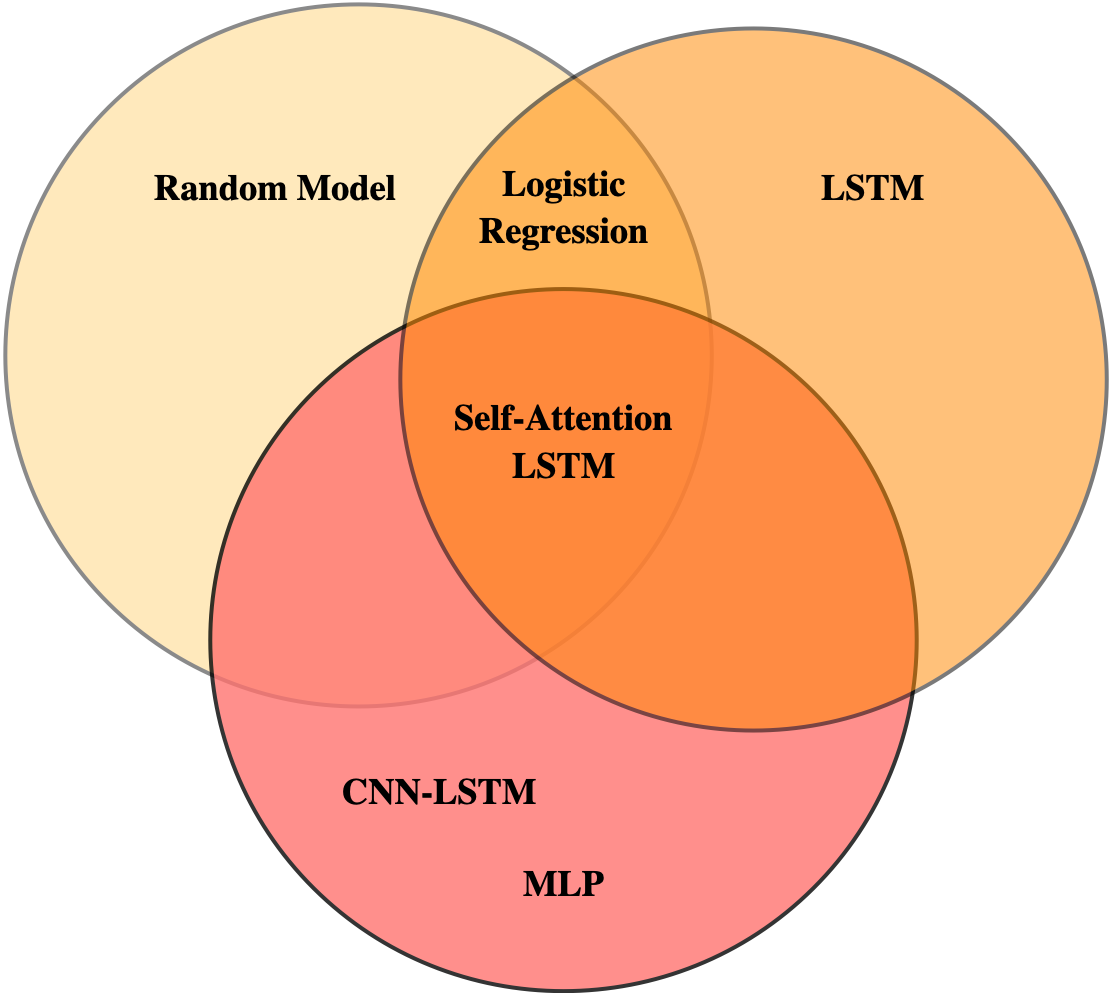
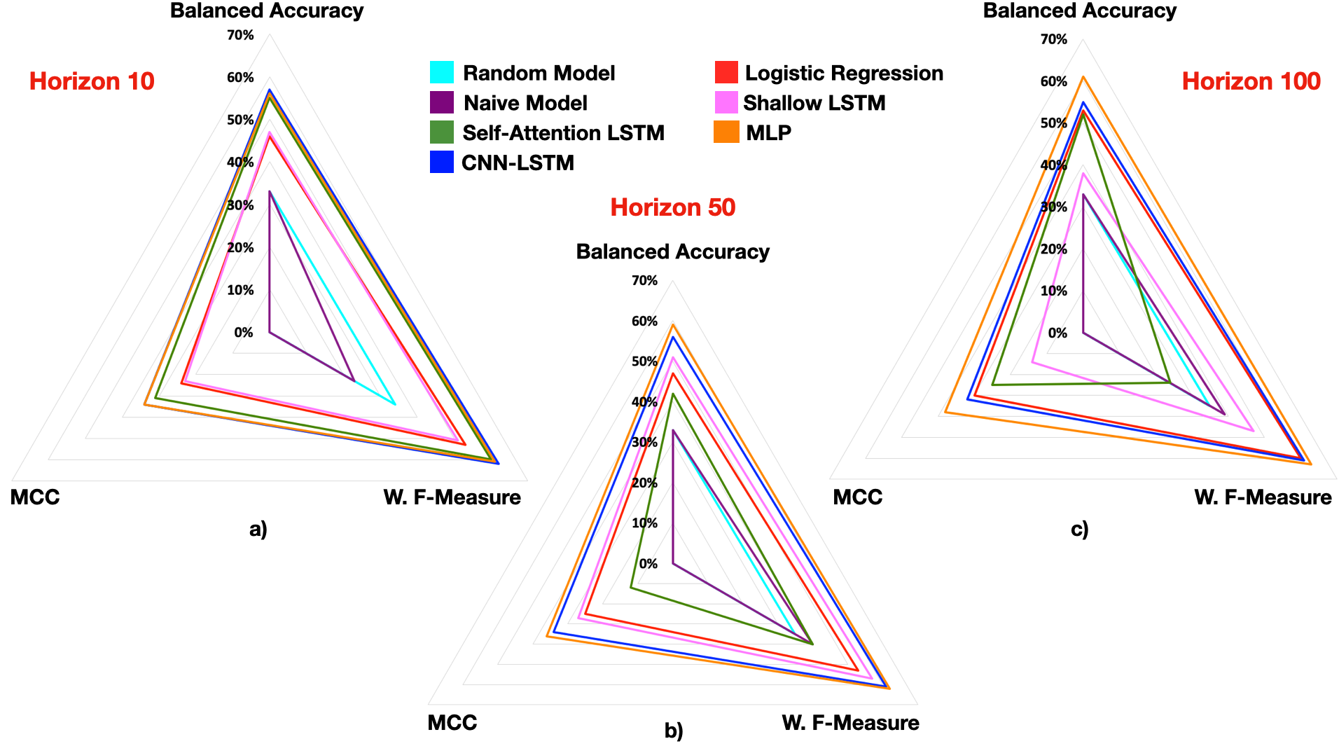
Out of sample performance metrics are reported in Table 7 and visualised in Figure 4. Models are clustered into three groups, based on their performance metrics. Specifically, in each one of these clusters it is possible to locate models that perform statistically equivalent throughout horizons , based on the MCC and weighted F-measure metrics described in Section 4.10. A representation of model clustering and ordering is presented in Figure 5, Appendix A.
Similarities between models’ performances are tested by means of the Bayesian Correlated t-test. This allowed to assign the models to the relative clusters or intersections of those as per the representation in Figure 5, Appendix A. It is important to clarify that the McNemar Test is not applied to compare models in this work, due to the belief that the Bayesian Correlated t-test is more appropriate for the present experimental setup. Further, from theoretical considerations, one expects to obtain analogous results to the presented Bayesian test. Future work shall include additional tests.
| Random Model | Naive Model | Logistic Regression | Shallow LSTM | Self-Attention LSTM | CNN-LSTM | Multilayer Perceptron | |||||||||||||||
| H10 | H50 | H100 | H10 | H50 | H100 | H10 | H50 | H100 | H10 | H50 | H100 | H10 | H50 | H100 | H10 | H50 | H100 | H10 | H50 | H100 | |
| Balanced Accuracy | 0.33 | 0.33 | 0.33 | 0.33 | 0.33 | 0.33 | 0.46 | 0.47 | 0.53 | 0.47 | 0.51 | 0.38 | 0.55 | 0.42 | 0.52 | 0.57 | 0.56 | 0.55 | 0.56 | 0.59 | 0.61 |
| Weighted Precision | 0.41 | 0.41 | 0.41 | 0.16 | 0.30 | 0.30 | 0.54 | 0.56 | 0.62 | 0.58 | 0.57 | 0.65 | 0.61 | 0.50 | 0.47 | 0.62 | 0.61 | 0.61 | 0.62 | 0.62 | 0.63 |
| Weighted Recall | 0.33 | 0.33 | 0.33 | 0.40 | 0.55 | 0.54 | 0.59 | 0.59 | 0.61 | 0.58 | 0.58 | 0.57 | 0.61 | 0.45 | 0.34 | 0.62 | 0.62 | 0.62 | 0.62 | 0.63 | 0.63 |
| Weighted F-Measure | 0.34 | 0.35 | 0.35 | 0.23 | 0.40 | 0.39 | 0.53 | 0.53 | 0.60 | 0.51 | 0.57 | 0.47 | 0.60 | 0.40 | 0.24 | 0.62 | 0.61 | 0.61 | 0.61 | 0.62 | 0.63 |
| Precision quantile [0, 0.25] | 0.26 | 0.26 | 0.26 | 0 | 0 | 0 | 0.57 | 0.57 | 0.57 | 0.57 | 0.56 | 0.58 | 0.60 | 0.37 | 0.55 | 0.59 | 0.59 | 0.59 | 0.59 | 0.59 | 0.59 |
| Precision quantile [0.25, 0.75] | 0.55 | 0.55 | 0.55 | 0.40 | 0.55 | 0.54 | 0.59 | 0.60 | 0.63 | 0.59 | 0.62 | 0.56 | 0.62 | 0.55 | 0.52 | 0.65 | 0.64 | 0.63 | 0.64 | 0.66 | 0.67 |
| Precision quantile [0.75, 1] | 0.20 | 0.20 | 0.20 | 0 | 0 | 0 | 0.31 | 0.38 | 0.58 | 0.57 | 0.43 | 0.97 | 0.57 | 0.52 | 0.26 | 0.57 | 0.57 | 0.57 | 0.59 | 0.58 | 0.57 |
| Recall quantile [0, 0.25] | 0.33 | 0.33 | 0.33 | 0 | 0 | 0 | 0.55 | 0.59 | 0.59 | 0.06 | 0.62 | 0.22 | 0.35 | 0.81 | 0.62 | 0.54 | 0.55 | 0.53 | 0.60 | 0.59 | 0.60 |
| Recall quantile [0.25, 0.75] | 0.33 | 0.33 | 0.33 | 1 | 1 | 1 | 0.82 | 0.81 | 0.76 | 0.85 | 0.69 | 0.93 | 0.76 | 0.44 | 0.01 | 0.71 | 0.72 | 0.74 | 0.74 | 0.70 | 0.68 |
| Recall quantile [0.75, 1] | 0.33 | 0.33 | 0.33 | 0 | 0 | 0 | 0 | 0 | 0.23 | 0.51 | 0.23 | 0 | 0.53 | 0.004 | 0.92 | 0.46 | 0.42 | 0.39 | 0.34 | 0.46 | 0.54 |
| F-Measure quantile [0, 0.25] | 0.29 | 0.29 | 0.29 | 0 | 0 | 0 | 0.56 | 0.57 | 0.58 | 0.11 | 0.59 | 0.31 | 0.44 | 0.503 | 0.58 | 0.57 | 0.57 | 0.56 | 0.59 | 0.59 | 0.59 |
| F-Measure quantile [0.25, 0.75] | 0.42 | 0.42 | 0.42 | 0.57 | 0.71 | 0.70 | 0.70 | 0.70 | 0.68 | 0.69 | 0.65 | 0.70 | 0.68 | 0.489 | 0.02 | 0.68 | 0.68 | 0.68 | 0.69 | 0.68 | 0.67 |
| F-Measure quantile [0.75, 1] | 0.25 | 0.25 | 0.25 | 0 | 0 | 0 | 0 | 0 | 0.33 | 0.54 | 0.30 | 0 | 0.55 | 0.009 | 0.40 | 0.51 | 0.48 | 0.46 | 0.43 | 0.51 | 0.56 |
| MCC | 0 | 0 | 0 | 0 | 0 | 0 | 0.24 | 0.25 | 0.30 | 0.23 | 0.27 | 0.14 | 0.31 | 0.120 | 0.25 | 0.34 | 0.34 | 0.32 | 0.34 | 0.36 | 0.38 |
| Cohen’s Kappa | 0 | 0 | 0 | 0 | 0 | 0 | 0.21 | 0.22 | 0.30 | 0.20 | 0.27 | 0.10 | 0.30 | 0.105 | 0.16 | 0.34 | 0.33 | 0.32 | 0.33 | 0.36 | 0.38 |
6 Discussion
This section builds upon the results in Section 5 and delves deeper into the analysis of model similarities and individual dimension-based model performances. A better Deep Learning-based understanding of LOB dynamics and modeling applications emerges from this.
Delving deeper into the analysis of model performances, the plots for the different prediction horizons in Figure 4 show how the MLP outperforms the CNN-LSTM throughout metrics and horizons (or performs analogously). A second group of models is represented by Logistic Regression and Shallow LSTM for horizons . The simplicity and stability of the Logistic Regression model benefits performance in where it performs analogously to the CNN-LSTM model. This is due to the CNN-LSTM model showing worsened performance, with respect to the MLP, for the longest horizon. A similar statement on depleted performance applies to the Shallow LSTM at this horizon. The Self-Attention LSTM performs well at , perhaps benefiting from the collective overview in the noisy shorter horizon, but sees significantly worse and unstable performance for the longer horizons. All stably performing models perform well above the two baseline models (Random and Naive), hence showing the ability of the model to learn and the possibility to extract information from the complex and highly stochastic setting which characterises the LOB. It is important to note that the MLP’s performance slightly increases with horizon length, showing how meaningful features are being extracted such that the model benefits from longer-term trajectories less affected by HFT short-term price noise.
We now analyse the model clusters in Figure 5, Appendix A. The clusters are formed using the Bayesian Correlated t-test described by Benavoli et al. [4]. Models are considered statistically equivalent and hence assigned to the same cluster on the basis of their MCC and weighted F-measure metrics.
The first cluster of models is characterised by the Random Model, and it also comprises Logistic Regression and Self-Attention LSTM at intersections with other groups. Looking at Table 7, low values for weighted Precision and weighted Recall are observed for the Random Model. This means that the system, for each horizon , yields balanced predictions throughout classes and by chance a few of them are correct. Most of the correctly classified labels belong to the central quantile , as shown by the higher values of its class-specific Precision. The second most correctly predicted quantile is the lower one , while the worst overall performance is associated with the upper quantile . Given that these predictions are picked randomly from an uniform distribution, the obtained results reflect the test set class distribution. The MCC and the Cohen’s Kappa are both equal to zero, thereby confirming that the model performs in a random fashion. Analogous considerations can be made for the Naive Model.
It results difficult to assign multinomial Logistic Regression to a cluster, as results in Table 7 show that the model is solid throughout horizons but lacks the ability to produce complex features which could improve its performance, due to the absence of non-linearities and hidden layers. Because of its behaviour, it is placed at the overlap between the first two clusters. Looking at Tables 8 and 9, it is possible to note how the multinomial Logistic Regression consistently outperforms the Random Model. For longer horizons (i.e. ), Logistic Regression
outperforms more structured Deep Learning models designed to handle specific dynamics. Despite this result, the model is systematically unable to decode the signal related to the upper quantile, perhaps due to the slight class imbalance in the training set.
The second cluster of models is represented by the shallow LSTM model. In this case, weighted Precision and weighted Recall values for all three horizons are higher than for Logistic Regression and the Random Model. This means that the proposed model is able to correctly predict a considerably high number of samples from different classes, when compared to the previously considered architectures. Similarly to what described in the previous paragraph, the model’s predictions are well balanced between quantiles, for horizons . This observation is confirmed by higher values for the MCC and Cohen’s Kappa for , which indicate that an increasing number of predictions match the ground-truth. Performance metrics collapse for the longer horizon in the upper quantile .
Results achieved by the Attention-LSTM make assigning the model to one of the three clusters
extremely difficult. As stated for class specific performances in the shallow LSTM model, there is a strong relation between metrics and the considered horizon . For , higher values of weighted Precision are accompanied by higher values of weighted Recall. These imply that the model is able to correctly predict a considerable number of samples from different classes. The only exception is represented by the lower quantile which has a lower class-specific weighted Recall. Looking at Table 7, it is possible to note higher MCC and Cohen’s Kappa values for the considered model, suggesting a relatively structured agreement between predictions and the ground truth, as described in Table 8. This makes the Attention-LSTM model statistically equivalent to the state-of-the-art models (namely the CNN-LSTM and MLP).
Our analysis changes significantly when considering . A decrease of more than in all performance metrics is observed. The greatest impact is on the upper quantile where the model is less capable to perform correct predictions. All these considerations strongly impact the Matthews Correlation Coefficient which has a value lower than the one for . The last analysis concerns the results obtained for . For this horizon, the model yields more balanced performances in terms of correctly predicted samples for the extreme quantiles , while the greatest impact in terms of performance is on . It is relevant to highlight the high number of misclassifications of the central quantile in favour of the upper one . Analysing results in Tables 8 and 9, it is possible to note that there is no reason to place the current experiment in the same cluster as the Shallow-LSTM, as they are never statistically equivalent. It is clear that for different horizons , the model shows completely different behaviours. For horizon it is statistically equivalent to the state-of-the-art methods which will be described in the next paragraph, but for there is no similarity to these models. This is the reason why the Attention-LSTM model is placed at the intersection of all clusters.
General performances for CNN-LSTM and MLP models are comparable to the ones for horizon in the Shallow-LSTM model. The difference with the Shallow-LSTM experiment, making CNN-LSTM and MLP models state-of-the-art, must be searched in their ability to maintain stable, high performances throughout horizons . Here too the higher values of weighted precision and recall for both the considered models, indicate the ability to correctly classify a significant number of samples associated with different target classes. Such an ability not only concerns higher level performance metrics, but is reflected in fine-grained per-class performance metrics as well. For different horizons , homogeneous class-specific weighted precision and recall are observed. The greater ability of these two models to correctly predict test samples is also shown by their highest values for Matthews Correlation Coefficient and Cohen’s Kappa, indicating a better overlap between predictions and the ground truth. A statistical equivalence between these models throughout metrics and horizons arises from the results presented in Tables 8 and 9.
|
|
|
||||||
|---|---|---|---|---|---|---|---|---|
| Self-Attention LSTM |
|
Multinomial Logistic Regression | ||||||
|
Self-Attention LSTM | Self-Attention LSTM | ||||||
|
|
Shallow LSTM | ||||||
| Random Model |
|
|
Multilayer Perceptron | |||||
|---|---|---|---|---|---|---|---|
|
Shallow LSTM |
|
|||||
| Naive Model | Multinomial Logistic Regression | Shallow LSTM | |||||
| Random Model | Self-Attention LSTM | Self-Attention LSTM | |||||
| Naive Model | Naive Model | ||||||
| Random Model | Random Model |
7 Conclusions
In the present work, different Deep Learning models are applied to the task of price return forecasting in financial markets based on the Limit Order Book. LOBSTER data is used to train and test the Deep Learning models which are then analysed in terms of results, similarities between the models, performance ranking and dynamics-based model embedding. Hypotheses regarding the nature of the Limit Order Book and its dynamics are then discussed on the basis of model performances and similarities.
The three main contributions of the present work are summarised hereafter and directions for future work are suggested.
The Multinomial Logistic Regression model is solid throughout horizons but lacks the ability to produce complex features which could improve its performance as well as explicit dynamics modeling. Not all complex architectures are though able to outperform the Multinomial Logistic Regression model, such as the shallow LSTM model. This architecture incorporates the temporal dimension alone and does not significantly outperform the Logistic Regression, yielding a decrease in predictive power for longer horizons (i.e. ). The time dimension, upon which recurrent models are based, is also exploited by the Self-Attention LSTM model, which is augmented by the Self-Attention module. This allows to consider the whole context, while calculating the relevance of specific components. This shrewdness guarantees state-of-the-art performances (in line with the CNN-LSTM and MLP) for short-range horizons (i.e. ).
This result then leads to the second consideration. It is clear that multiple levels of complexity in terms of return prediction exist in an LOB. There are at least two levels of complexity. The first one relates to short-range predictions (i.e. horizon ). It is time dependent and can be well predicted by statically considering spatial dynamics which can be found in the immediate history (the context) related to the LOB state at tick time t. The second level of complexity is related to longer-range predictions (i.e. horizons ) and multiple dimensions (temporal and spatial) must be taken into account to interpret it. The CNN-LSTM model, which explicitly models both dynamics, seems to penetrate deeper LOB levels of complexity guaranteeing stable and more accurate predictions for longer horizons too. This finding, combined with the results previously discussed, would lead to assert that space and time could be building blocks of the LOB’s inner structure. This hypothesis is though partially denied by the statistically equivalent performance of the Multilayer Perceptron.
The last consideration hence follows from this. It is observed that a simple Multilayer Perceptron, which does not explicitly model temporal or spatial dynamics, yields statistically equivalent results to the CNN-LSTM model, the current state-of-the-art. According to these results, it is possible to conclude that both time and space are a good approximations of the underlying LOB’s dimensions for the different prediction horizons , but they should not be considered the real, necessary underlying dimensions ruling this entity and hence the market.
It is important to carry over some important considerations made throughout the paper which put the work into context and lead to future work. In the present work we investigate price change-based horizons, which hence correct for market volatlity. Future works should investigate the more difficult and noisy - but very insightful in practice - task of predicting with “real time” horizons. The MLP used here is passed the same historical data as temporal models - per its structure it does not encode sequentiality (which the model could through infer), but we do not make any statements about the near LOB history being negligible. The considered stock falls into the category of large tick stocks which are vastly investigated in the literature and are know to be more suitable for ML-based predictions than small tick ones. Future work should investigate a now overdue framework for ML-based prediction in small tick stocks with state of the art performance comparable to that achieved on large tick stocks.
The present work has demonstrated how Deep Learning can serve a theoretical and interpretative purpose in financial markets. Future works should further explore Deep Learning-based theoretical investigations of financial markets and trading dynamics. The upcoming paper by the authors of this work presents an extension of the concepts in this work to Deep Reinforcement Learning and calls for further theoretical agent-based work in the field of high frequency trading and market making.
8 Acknowledgements
The authors acknowledge Riccardo Marcaccioli for the useful discussions and suggestions which have improved the quality of this work and sparked directions for future work. AB acknowledges support from the European Erasmus+ Traineeship Program. TA and JT acknowledge support from the EC Horizon 2020 FIN-Tech (H2020-ICT-2018-2 825215) and EPSRC (EP/L015129/1). TA also acknowledges support from ESRC (ES/K002309/1); EPSRC (EP/P031730/1).
References
- [1] F. Abergel et al. “Limit Order Books”, PHYSICS OF SOCIETY: ECONOPHYSICS Cambridge University Press, 2016 URL: https://books.google.co.uk/books?id=5JIrDAAAQBAJ
- [2] Ethem Alpaydm “Combined 5 2 cv F test for comparing supervised classification learning algorithms” In Neural computation 11.8 MIT Press, 1999, pp. 1885–1892
- [3] Ron Artstein and Massimo Poesio “Inter-coder agreement for computational linguistics” In Computational Linguistics 34.4 MIT Press, 2008, pp. 555–596
- [4] Alessio Benavoli, Giorgio Corani, Janez Demšar and Marco Zaffalon “Time for a change: a tutorial for comparing multiple classifiers through Bayesian analysis” In The Journal of Machine Learning Research 18.1 JMLR. org, 2017, pp. 2653–2688
- [5] James O Berger and Thomas Sellke “Testing a point null hypothesis: The irreconcilability of p values and evidence” In Journal of the American statistical Association 82.397 Taylor & Francis Group, 1987, pp. 112–122
- [6] Jean-Philippe Bouchaud, J Doyne Farmer and Fabrizio Lillo “How markets slowly digest changes in supply and demand” In Handbook of financial markets: dynamics and evolution Elsevier, 2009, pp. 57–160
- [7] Antonio Briola and Jeremy David Turiel “CNN-LSTM_Limit_Order_Book: Third Release” Zenodo, 2020 DOI: 10.5281/zenodo.4104275
- [8] Arno Candel, Viraj Parmar, Erin LeDell and Anisha Arora “Deep learning with H2O” In H2O. ai Inc, 2016
- [9] Francois Chollet “Deep learning with Python” Manning Publications Company, 2017
- [10] François Chollet “Keras”, https://keras.io, 2015
- [11] Jacob Cohen “A coefficient of agreement for nominal scales” In Educational and psychological measurement 20.1 Sage Publications Sage CA: Thousand Oaks, CA, 1960, pp. 37–46
- [12] Giorgio Corani and Alessio Benavoli “A Bayesian approach for comparing cross-validated algorithms on multiple data sets” In Machine Learning 100.2-3 Springer, 2015, pp. 285–304
- [13] Janez Demšar “On the appropriateness of statistical tests in machine learning” In Workshop on Evaluation Methods for Machine Learning in conjunction with ICML, 2008, pp. 65
- [14] James Dickey “Scientific reporting and personal probabilities: Student’s hypothesis” In Journal of the Royal Statistical Society: Series B (Methodological) 35.2 Wiley Online Library, 1973, pp. 285–305
- [15] Thomas G Dietterich “Approximate statistical tests for comparing supervised classification learning algorithms” In Neural computation 10.7 MIT Press, 1998, pp. 1895–1923
- [16] Ward Edwards, Harold Lindman and Leonard J Savage “Bayesian statistical inference for psychological research.” In Psychological review 70.3 American Psychological Association, 1963, pp. 193
- [17] Sumitra Ganesh et al. “Reinforcement Learning for Market Making in a Multi-agent Dealer Market” In arXiv preprint arXiv:1911.05892, 2019
- [18] Jan Gorodkin “Comparing two K-category assignments by a K-category correlation coefficient” In Computational biology and chemistry 28.5-6 Elsevier, 2004, pp. 367–374
- [19] William H Greene “Econometric analysis” Pearson Education India, 2003
- [20] Isabelle Guyon et al. “Design of the 2015 chalearn automl challenge” In 2015 International Joint Conference on Neural Networks (IJCNN), 2015, pp. 1–8 IEEE
- [21] Isabelle Guyon et al. “Analysis of the AutoML Challenge series 2015-2018” In AutoML, Springer series on Challenges in Machine Learning, 2019
- [22] Simon Haykin and Neural Network “A comprehensive foundation” In Neural networks 2.2004, 2004, pp. 41
- [23] Sepp Hochreiter and Jürgen Schmidhuber “Long short-term memory” In Neural computation 9.8 MIT Press, 1997, pp. 1735–1780
- [24] Ruihong Huang and Tomas Polak “LOBSTER: Limit order book reconstruction system” In Available at SSRN 1977207, 2011
- [25] Nathalie Japkowicz and Mohak Shah “Evaluating learning algorithms: a classification perspective” Cambridge University Press, 2011
- [26] Michael Kearns and Yuriy Nevmyvaka “Machine learning for market microstructure and high frequency trading” In High Frequency Trading: New Realities for Traders, Markets, and Regulators, 2013
- [27] John D Kelleher, Brian Mac Namee and Aoife D’arcy “Fundamentals of machine learning for predictive data analytics: algorithms, worked examples, and case studies” MIT press, 2015
- [28] Diederik P Kingma and Jimmy Ba “Adam: A method for stochastic optimization” In arXiv preprint arXiv:1412.6980, 2014
- [29] Yann LeCun and Yoshua Bengio “Convolutional networks for images, speech, and time series” In The handbook of brain theory and neural networks 3361.10, 1995, pp. 1995
- [30] Xiaoxiao Li, Joao Saude, Prashant Reddy and Manuela Veloso “Classifying and Understanding Financial Data Using Graph Neural Network”, 2020
- [31] Zachary C Lipton, John Berkowitz and Charles Elkan “A critical review of recurrent neural networks for sequence learning” In arXiv preprint arXiv:1506.00019, 2015
- [32] Lawrence Mosley “A balanced approach to the multi-class imbalance problem”, 2013
- [33] Claude Nadeau and Yoshua Bengio “Inference for the generalization error” In Advances in neural information processing systems, 2000, pp. 307–313
- [34] F. Pedregosa et al. “Scikit-learn: Machine Learning in Python” In Journal of Machine Learning Research 12, 2011, pp. 2825–2830
- [35] Steven L Salzberg “On comparing classifiers: Pitfalls to avoid and a recommended approach” In Data mining and knowledge discovery 1.3 Springer, 1997, pp. 317–328
- [36] Justin A Sirignano “Deep learning for limit order books” In Quantitative Finance 19.4 Taylor & Francis, 2019, pp. 549–570
- [37] Justin Sirignano and Rama Cont “Universal features of price formation in financial markets: perspectives from deep learning” In Quantitative Finance 19.9 Taylor & Francis, 2019, pp. 1449–1459
- [38] Avraam Tsantekidis et al. “Forecasting stock prices from the limit order book using convolutional neural networks” In 2017 IEEE 19th Conference on Business Informatics (CBI) 1, 2017, pp. 7–12 IEEE
- [39] Ashish Vaswani et al. “Attention is all you need” In Advances in neural information processing systems, 2017, pp. 5998–6008
- [40] Pauli Virtanen et al. “SciPy 1.0: Fundamental Algorithms for Scientific Computing in Python” In Nature Methods 17, 2020, pp. 261–272 DOI: https://doi.org/10.1038/s41592-019-0686-2
- [41] Ian H Witten, Eibe Frank and Mark A. Hall “Data Mining: Practical Machine Learning Tools and Techniques” Morgan Kaufmann, 2016
- [42] Z. Zhang, S. Zohren and S. Roberts “DeepLOB: Deep Convolutional Neural Networks for Limit Order Books” In IEEE Transactions on Signal Processing 67.11, 2019, pp. 3001–3012 DOI: 10.1109/TSP.2019.2907260
- [43] Zihao Zhang, Stefan Zohren and Stephen Roberts “Bdlob: Bayesian deep convolutional neural networks for limit order books” In arXiv preprint arXiv:1811.10041, 2018
- [44] Zihao Zhang, Stefan Zohren and Stephen Roberts “Extending deep learning models for limit order books to quantile regression” In arXiv preprint arXiv:1906.04404, 2019
Appendix A Bayesian-based model clustering