This paper was converted on www.awesomepapers.org from LaTeX by an anonymous user.
Want to know more? Visit the Converter page.

Deep Neural Networks are Adaptive to Function Regularity and Data Distribution in Approximation and Estimation

Hao Liu Jiahui Cheng Wenjing Liao Hao Liu is affiliated with the Math department of Hong Kong Baptist University; Jiahui Cheng and Wenjing Liao are affiliated with the School of Math at Georgia Tech; Email: haoliu@hkbu.edu.hk, {\{jcheng328, wliao60}\}@gatech.edu. This research is partially supported by National Natural Science Foundation of China 12201530, HKRGC ECS 22302123, HKBU 179356, NSF DMS–2012652, NSF DMS-2145167 and DOE SC0024348.
Abstract

Deep learning has exhibited remarkable results across diverse areas. To understand its success, substantial research has been directed towards its theoretical foundations. Nevertheless, the majority of these studies examine how well deep neural networks can model functions with uniform regularity. In this paper, we explore a different angle: how deep neural networks can adapt to different regularity in functions across different locations and scales and nonuniform data distributions. More precisely, we focus on a broad class of functions defined by nonlinear tree-based approximation. This class encompasses a range of function types, such as functions with uniform regularity and discontinuous functions. We develop nonparametric approximation and estimation theories for this function class using deep ReLU networks. Our results show that deep neural networks are adaptive to different regularity of functions and nonuniform data distributions at different locations and scales. We apply our results to several function classes, and derive the corresponding approximation and generalization errors. The validity of our results is demonstrated through numerical experiments.

1 Introduction

Deep learning has achieved significant success in practical applications with high-dimensional data, such as computer vision (Krizhevsky et al., 2012), natural language processing (Graves et al., 2013; Young et al., 2018), health care (Miotto et al., 2018; Jiang et al., 2017) and bioinformatics (Alipanahi et al., 2015; Zhou and Troyanskaya, 2015). The success of deep learning demonstrates the power of neural networks in representing and learning complex operations on high-dimensional data.

In the past decades, the representation power of neural networks has been extensively studied. Early works in literature focused on shallow (two-layer) networks with continuous sigmoidal activations (a function σ(x)\sigma(x) is sigmoidal, if σ(x)0\sigma(x)\rightarrow 0 as xx\rightarrow-\infty, and σ(x)1\sigma(x)\rightarrow 1 as xx\rightarrow\infty) for a universal approximation of continuous functions in a unit hypercube (Irie and Miyake, 1988; Funahashi, 1989; Cybenko, 1989; Hornik, 1991; Chui and Li, 1992; Leshno et al., 1993; Barron, 1993; Mhaskar, 1996). The universal approximation theory of feedforward neural networks with a ReLU activation σ(x)=max(0,x)\sigma(x)=\max(0,x) was studied in Lu et al. (2017); Hanin (2017); Daubechies et al. (2022); Yarotsky (2017); Schmidt-Hieber (2017); Suzuki (2018). In particular, the approximation theories of ReLU networks have been established for the Sobolev Wk,W^{k,\infty} (Yarotsky, 2017), Hölder (Schmidt-Hieber, 2017) and Besov (Suzuki, 2018) functions. These works guarantee that, the Sobolev, Hölder, or Besov function class can be well approximated by a ReLU network function class with a properly chosen network architecture. The approximation error in these works was given in terms of certain function norm. Furthermore, the works in Gühring et al. (2020); Hon and Yang (2021); Liu et al. (2022a) proved the approximation error in terms of the Sobelev norm, which guaranteed the approximation error for the function and its derivatives simultaneously. In terms of the network architecture, feedforward neural networks were considered in the vast majority of approximation theories. Convolutional neural networks were considered in Zhou (2020); Petersen and Voigtlaender (2020), and convolutional residual networks were considered in Oono and Suzuki (2019); Liu et al. (2021).

It has been widely believed that deep neural networks are adaptive to complex data structures. Recent progresses have been made towards theoretical justifications that deep neural networks are adaptive to low-dimensional structures in data. Specifically, function approximation theories have been established for Hölder and Sobolev functions supported on low-dimensional manifolds (Chen et al., 2019a; Schmidt-Hieber, 2019; Cloninger and Klock, 2020; Nakada and Imaizumi, 2020; Liu et al., 2021). The network size in these works crucially depends on the intrinsic dimension of data, instead of the ambient dimension. In the task of regression and classification, the sample complexity of neural networks (Chen et al., 2019b; Nakada and Imaizumi, 2020; Liu et al., 2021) depends on the intrinsic dimension of data, while the ambient dimension does not affect the rate of convergence.

This paper answers another interesting question about the adaptivity of deep neural networks: How does deep neural networks adapt to the function regularity and data distribution at different locations and scales? The answer of this question is beyond the scope of existing function approximation and estimation theory of neural networks. The Sobolev Wk,W^{k,\infty} and Hölder functions are uniformly regular within the whole domain. The analytical technique to build the approximation theory of these functions relies on accurate local approximations everywhere within the domain. In real applications, functions of interests often exhibit different regularity at different locations and scales. Empirical experiments have demonstrated that deep neural networks are capable of extracting interesting information at various locations and scales (Chung et al., 2016; Haber et al., 2018). However, there are limited works on theoretical justifications of the adaptivity of neural networks.

In this paper, we re-visit the nonlinear approximation theory (DeVore, 1998) in the classical multi-resolution analysis (Mallat, 1999; Daubechies, 1992). Nonlinear approximations allow one to approximate functions beyond linear spaces. The smoothness of the function can be defined according to the rate of approximation error versus the complexity of the elements. In many settings, such characterization of smoothness is significantly weaker than the uniform regularity condition in the Sobolev or Hölder class (DeVore, 1998).

We focus on the tree-based nonlinear approximations with piecewise polynomials (Binev et al., 2007, 2005; Cohen et al., 2001). Specifically, the domain of functions is partitioned to multiscale dyadic cubes associated with a master tree. If we build piecewise polynomials on these multiscale dyadic cubes, we naturally obtain multiscale piecewise polynomial approximations. A refinement quantity is defined at every node to quantify how much the error decreases when the node is refined to its children. A thresholding of the master tree based on this refinement quantity gives rise to a truncated tree, as well as an adaptive partition of the domain. Thanks to the thresholding technique, we can define a function class whose regularity is characterized by how fast the size of the truncated tree grows with respect to the level of the threshold. This is a large function class containing the Hölder and piecewise Hölder functions as special cases.

Our main contributions can be summarized as:

  1. 1.

    We establish the approximation theory of deep ReLU networks for a large class of functions whose regularity is defined according to the nonlinear tree-based approximation theory. This function class allows the regularity of the function to vary at different locations and scales.

  2. 2.

    We provide several examples of functions in this class which exhibit different information at different locations and scales. These examples are beyond the characterization of function classes with uniform regularity, such as the Hölder class.

  3. 3.

    A nonparametric estimation theory for this large function class is established with deep ReLU networks, which is validated by numerical experiments.

  4. 4.

    Our results demonstrate that, when deep neural networks are representing functions, it does not require a uniform regularity everywhere on the domain. Deep neural networks are automatically adaptive to the regularity of functions at different locations and scales.

In literature, adaptive function approximation and estimation has been studied for classical methods (DeVore, 1998), including free-knot spline (Jupp, 1978), adaptive smoothing splines (Wahba, 1995; Pintore et al., 2006; Liu and Guo, 2010; Wang et al., 2013), nonlinear wavelet (Cohen et al., 2001; Donoho and Johnstone, 1998; Donoho et al., 1995), and adaptive piecewise polynomial approximation (Binev et al., 2007, 2005). Based on traditional methods for estimating functions with uniform regularity, these methods allow the smoothing parameter, the kernel band width or knots placement to vary spatially to adapt to the varying regularity. Kernel methods with variable bandwidth were studied in Muller and Stadtmuller (1987) and local polynomial estimators were studied in Fan and Gijbels (1996). Based on traditional smoothing splines with a global smoothing parameter, Wahba (1995) suggested to replace the smoothing parameter by a roughness penalty function. This idea was then studied in Pintore et al. (2006); Liu and Guo (2010) by using piecewise constant roughness penalty, and in Wang et al. (2013) with a more general roughness penalty. A locally penalized spline estimator was proposed and studied in Ruppert and Carroll (2000), in which a penalty function was applied to spline coefficients and was knot-dependent. Adaptive wavelet shrinkage was studied in Donoho and Johnstone (1994, 1995, 1998), in which the authors used selective wavelet reconstruction, adaptive thresholding and nonlinear wavelet shrinkage to achieve adaptation to spatially varying regularity, and proved the minimax optimality. A Bayesian mixture of splines method was proposed in Wood et al. (2002), in which each component spline had a locally defined smoothing parameter. Other methods include regression splines (Fridedman, 1991; Smith and Kohn, 1996; Denison et al., 1998), hybrid smoothing splines and regression splines (Luo and Wahba, 1997), and the trend filtering method (Tibshirani, 2014). The minimax theory for adaptive nonparametric estimator was established in Cai (2012). Most of the works mentioned above focused on one-dimensional problems. For high dimensional problems, an additive model was considered in Ruppert and Carroll (2000). Recently, the Bayesian additive regression trees were studied in Jeong and Rockova (2023) for estimating a class of sparse piecewise heterogeneous anisotropic Hölder continuous functions in high dimension.

Classical methods mentioned above adapt to varying regularity of the target functions through a careful selection of some adaptive parameter, such as the location of knots, kernel bandwidth, roughness penalty and adaptive tree structure. These methods require the knowledge about or an estimation of how the regularity of the target function changes. Compared to classical methods, deep learning solves the regression problem by minimizing the empirical risk in (20), so the same optimization problem can be applied to various functions without explicitly figuring out where the regularity of the underlying function changes. Such kind of automatic adaptivity is crucial for real-world applications.

The connection between neural networks and adaptive spline approximation has been studied in Daubechies et al. (2022); DeVore et al. (2021); Liu et al. (2022b); Petersen and Voigtlaender (2018); Imaizumi and Fukumizu (2019). In particular, an adaptive network enhancement method was proposed in Liu et al. (2022b) for the best least-squares approximation using two-layer neural networks. The adaptivity of neural networks to data distributions was considered in Zhang et al. (2023), where the concept of an effective Minkowski dimension was introduced and applied to anisotropic Gaussian distributions. The approximation error and generalization error for learning piecewise Hölder functions in d\mathbb{R}^{d} are developed in Petersen and Voigtlaender (2018) and Imaizumi and Fukumizu (2019), respectively. In the settings of Petersen and Voigtlaender (2018) and Imaizumi and Fukumizu (2019), each discontinuity boundary is parametrized by a (d1)(d-1)-dimensional Hölder function, which is called a horizon function. In this paper, we consider a function class based on nonlinear tree-based approximation, and provide approximation and generalization theories of deep neural networks for this function class, as well as several examples related with practical applications, which are not implied by existing works. For piecewise Hölder functions, our setting only assumes the boundary of each piece has Minkowski dimension d1d-1, which is more general than that considered in Petersen and Voigtlaender (2018); Imaizumi and Fukumizu (2019), see Section 4.3.3 and 4.5.3 for more detailed discussions.

Our paper is organized as follows: In Section 2, we introduce notations and concepts used in this paper. Tree based adaptive approximation and some examples are presented in Section 3. We present our main results, the adaptive approximation and generalization theories of deep neural networks in Section 4, and the proofs are deferred to Section 6. Our theories is validated by numerical experiments in Section 5. This paper is concluded in Section 7.

2 Notation and Preliminaries

In this section, we introduce our notation, some preliminary definitions and ReLU networks.

2.1 Notation

We use normal lower case letters to denote scalars, and bold lower case letters to denote vectors. For a vector 𝐱d\mathbf{x}\in\mathbb{R}^{d}, we use xix_{i} to denote the ii-th entry of 𝐱\mathbf{x}. The standard 2-norm of 𝐱\mathbf{x} is 𝐱2=(i=1dxi2)12\|\mathbf{x}\|_{2}=(\sum_{i=1}^{d}x_{i}^{2})^{\frac{1}{2}}. For a scalar a>0a>0, a\lfloor a\rfloor denotes the largest integer that is no larger than aa, a\lceil a\rceil denotes the smallest integer that is no smaller than aa. Let II be a set. We use χI\chi_{I} to denote the indicator function on II such that χI(𝐱)=1\chi_{I}(\mathbf{x})=1 if 𝐱I\mathbf{x}\in I and χI(𝐱)=0\chi_{I}(\mathbf{x})=0 if 𝐱I\mathbf{x}\notin I. The notation #I\#I denotes the cardinality of II.

Denote the domain X=[0,1]dX=[0,1]^{d}. For a function f:Xf:X\rightarrow\mathbb{R} and a multi-index 𝜶=[α1,,αd]\bm{\alpha}=[\alpha_{1},\dots,\alpha_{d}]^{\top}, 𝜶f\partial^{\bm{\alpha}}f denotes |𝜶|f/x1α1xdαd\partial^{|\bm{\alpha}|}f/\partial x_{1}^{\alpha_{1}}\cdots\partial x_{d}^{\alpha_{d}}, where |𝜶|=k=1dαk|\bm{\alpha}|=\sum_{k=1}^{d}\alpha_{k}. We denote 𝒙𝜶=x1α1x2α2xdαd\bm{x}^{\bm{\alpha}}=x_{1}^{\alpha_{1}}x_{2}^{\alpha_{2}}\cdots x_{d}^{\alpha_{d}}. Let ρ\rho be a measure on XX. The L2L^{2} norm of ff with respect to the measure ρ\rho is fL2(ρ)2=X|f(𝐱)|2𝑑ρ\|f\|^{2}_{L^{2}(\rho)}=\int_{X}|f(\mathbf{x})|^{2}d\rho. We say fL2(ρ)f\in L^{2}(\rho) if fL2(ρ)2<\|f\|^{2}_{L^{2}(\rho)}<\infty. We denote fL2(ρ(Ω))2=Ω|f(𝐱)|2𝑑ρ\|f\|_{L^{2}(\rho(\Omega))}^{2}=\int_{\Omega}|f(\mathbf{x})|^{2}d\rho for any ΩX\Omega\subset X.

The notation of fgf\lesssim g means that there exists a constant CC independent of any variable upon which ff and gg depend, such that fCgf\leq Cg; similarly for \gtrsim. fgf\asymp g means that fgf\lesssim g and fgf\gtrsim g.

2.2 Preliminaries

Definition 1 (Hölder functions).

A function f:Xf:X\rightarrow\mathbb{R} belongs to the Hölder space r(X)\mathcal{H}^{r}(X) with a Hölder index r>0r>0, if

fr(X)\displaystyle\|f\|_{\mathcal{H}^{r}(X)} =max|𝜶|<r1sup𝐱X|𝜶f(𝐱)|+max|𝜶|=r1sup𝐱𝐳X|𝜶f(𝐱)𝜶f(𝐳)|𝐱𝐳2rr1<.\displaystyle=\max_{|\bm{\alpha}|<\lceil r-1\rceil}\sup\limits_{\mathbf{x}\in X}|\partial^{\bm{\alpha}}f(\mathbf{x})|+\max\limits_{|\bm{\alpha}|=\lceil r-1\rceil}\sup\limits_{\mathbf{x}\neq\mathbf{z}\in X}\frac{|\partial^{\bm{\alpha}}f(\mathbf{x})-\partial^{\bm{\alpha}}f(\mathbf{z})|}{\|\mathbf{x}-\mathbf{z}\|_{2}^{r-\lceil r-1\rceil}}<\infty. (1)
Definition 2 (Minkowski dimension).

Let Ω[0,1]d\Omega\subset[0,1]^{d}. For any ε>0\varepsilon>0, 𝒩(ε,Ω,)\mathcal{N}(\varepsilon,\Omega,\|\cdot\|_{\infty}) denotes the fewest number of ε\varepsilon-balls that cover Ω\Omega in terms of \|\cdot\|_{\infty}. The (upper) Minkowski dimension of Ω\Omega is defined as

dM(Ω):=lim supε0+log𝒩(ε,Ω,)log(1/ε).d_{M}(\Omega):=\limsup_{\varepsilon\rightarrow 0^{+}}\frac{\log\mathcal{N}(\varepsilon,\Omega,\|\cdot\|_{\infty})}{\log(1/\varepsilon)}.

We further define the Minkowski dimension constant of Ω\Omega as

cM(Ω)=supε>0𝒩(ε,Ω,)εdM(Ω).c_{M}(\Omega)=\sup_{\varepsilon>0}\mathcal{N}(\varepsilon,\Omega,\|\cdot\|_{\infty})\varepsilon^{d_{M}(\Omega)}.

Such a constant is an upper bound on the rate of how 𝒩(ε,Ω,)\mathcal{N}(\varepsilon,\Omega,\|\cdot\|_{\infty}) scales with εdM(Ω)\varepsilon^{-d_{M}(\Omega)}.

ReLU network. In this paper, we consider the feedforward neural networks defined over in the form of

fNN(𝐱)=WLReLU(WL1ReLU(W1𝐱+𝐛1)++𝐛L1)+𝐛L,\displaystyle f_{\rm NN}(\mathbf{x})=W_{L}\cdot\mathrm{ReLU}\big{(}W_{L-1}\cdots\mathrm{ReLU}(W_{1}\mathbf{x}+\mathbf{b}_{1})+\cdots+\mathbf{b}_{L-1}\big{)}+\mathbf{b}_{L}, (2)

where WlW_{l}’s are weight matrices, 𝐛l\mathbf{b}_{l}’s are biases, and ReLU(a)=max{a,0}\mathrm{ReLU}(a)=\max\{a,0\} denotes the rectified linear unit (ReLU). Define the network class as

NN(L,w,K,κ,M)={fNN:d|fNN(𝐱) is in the form of (2) with L layers,\displaystyle\mathcal{F}_{\rm NN}(L,w,K,\kappa,M)=\big{\{}f_{\rm NN}:\mathbb{R}^{d}\rightarrow\mathbb{R}|f_{\rm NN}(\mathbf{x})\mbox{ is in the form of (\ref{eq.FNN.f}) with }L\mbox{ layers,} (3)
width bounded by w,fLM,Wl,κ,𝐛lκ, and l=1LWl0+𝐛l0K},\displaystyle\mbox{width bounded by }w,\|f\|_{L^{\infty}}\leq M,\ \|W_{l}\|_{\infty,\infty}\leq\kappa,\|\mathbf{b}_{l}\|_{\infty}\leq\kappa,\ \mbox{ and }\textstyle\sum_{l=1}^{L}\|W_{l}\|_{0}+\|\mathbf{b}_{l}\|_{0}\leq K\big{\}},

W,=maxi,j|Wi,j|,𝐛=maxi|bi|\|W\|_{\infty,\infty}=\max_{i,j}|W_{i,j}|,\ \|\mathbf{b}\|_{\infty}=\max_{i}|b_{i}| for any matrix WW and vector 𝐛\mathbf{b}, and 0\|\cdot\|_{0} denotes the number of nonzero elements of its argument.

3 Adaptive approximation

This section is an introduction to tree-based nonlinear approximation and a function class whose regularity is defined through nonlinear approximation theory. We re-visit tree-based nonlinear approximations and define this function class in Subsection 3.1. Several examples of this function class are given in Subsection 3.2.

3.1 Tree-Based Nonlinear Approximations

In the classical tree-based nonlinear approximations (Binev et al., 2007, 2005; Cohen et al., 2001), piecewise polynomials are used to approximate the target function on an adaptive partition. For simplicity, we focus on the case that the function domain is X=[0,1]dX=[0,1]^{d}. Let ρ\rho be a probability measure on XX and fL2(ρ)f\in L^{2}(\rho). The multiscale dyadic partitions of XX give rise to a tree structure. It is natural to consider nonlinear approximations based on this tree structure.

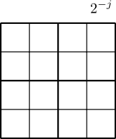
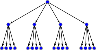
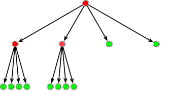
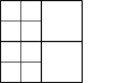
Let 𝒞j={Cj,k}k=12jd\mathcal{C}_{j}=\{C_{j,k}\}_{k=1}^{2^{jd}} be the collection of dyadic subcubes of XX of sidelength 2j2^{-j}. Here jj denotes the scale of Cj,kC_{j,k} with a small jj and kk denotes the location. A small jj represents the coarse scale, and a large jj represents the fine scale. These dyadic cubes are naturally associated with a tree 𝒯\mathcal{T}. Each node of this tree corresponds to a cube Cj,kC_{j,k}. The dyadic partition of the 2D cube [0,1]2[0,1]^{2} and its associated tree are illustrated in Figure 1. Every node Cj,kC_{j,k} at scale jj has 2d2^{d} children at scale j+1j+1. We denote the set of children of Cj,kC_{j,k} by 𝒞(Cj,k)\mathcal{C}(C_{j,k}). When the node Cj,kC_{j,k} is a child of the node Cj1,kC_{j-1,k^{\prime}}, we call Cj1,kC_{j-1,k^{\prime}} the parent of Cj,kC_{j,k}, denoted by 𝒫(Cj,k)\mathcal{P}(C_{j,k}). A proper subtree 𝒯0\mathcal{T}_{0} of 𝒯\mathcal{T} is a collection of nodes such that: (1) the root node XX is in 𝒯0\mathcal{T}_{0}; (2) if Cj,kXC_{j,k}\neq X is in 𝒯0\mathcal{T}_{0}, then its parent is also in 𝒯0\mathcal{T}_{0}. Given a proper subtree 𝒯0\mathcal{T}_{0} of 𝒯\mathcal{T}, the outer leaves of 𝒯0\mathcal{T}_{0} contain all Cj,k𝒯C_{j,k}\in\mathcal{T} such that Cj,k𝒯0C_{j,k}\notin\mathcal{T}_{0} but the parent of Cj,kC_{j,k} belongs to 𝒯0\mathcal{T}_{0}: Cj,k𝒯0C_{j,k}\notin\mathcal{T}_{0} but 𝒫(Cj,k)𝒯0\mathcal{P}(C_{j,k})\in\mathcal{T}_{0}. The collection of the outer leaves of 𝒯0\mathcal{T}_{0}, denoted by Λ=Λ(𝒯0)\Lambda=\Lambda(\mathcal{T}_{0}), forms a partition of XX.

Refer to caption
(a) Dyadic partition
Refer to caption
(b) Tree
Figure 1: The dyadic partition of the 2D unit cube [0,1]2[0,1]^{2} and the associated tree.

The tree-based nonlinear approximation generates an adaptive partition with a thresholding technique. In certain cases, this thresholding technique boils down to wavelet thresholding. Specifically, one defines a refinement quantity on each node of the tree, and then thresholds the tree to the smallest proper subtree containing all the nodes whose refinement quantity is above certain value. Adaptive partitions are given by the outer leaves of this proper subtree after thresholding.

We consider piecewise polynomial approximations of ff by polynomials of degree θ\theta, where θ\theta is a nonnegative integer. Let 𝒫θ\mathcal{P}_{\theta} be the space of dd-variable polynomials of degree no more than θ\theta. For any cube Cj,kC_{j,k}, the best polynomial approximating ff on Cj,kC_{j,k} is

pj,k=pj,k(f)=argminp𝒫θ(fp)χCj,kL2(ρ).p_{j,k}=p_{j,k}(f)=\mathop{\mathrm{argmin}}_{p\in\mathcal{P}_{\theta}}\|(f-p)\chi_{C_{j,k}}\|_{L^{2}(\rho)}. (4)

At a fixed scale jj, ff can be approximated by the piecewise polynomial fj=kpj,kχCj,kf_{j}=\sum_{k}p_{j,k}\chi_{C_{j,k}}. Denote VjV_{j} as the space of θ\theta-order piecewise polynomial functions on the partition kCj,k\cup_{k}C_{j,k}. By definition, VjV_{j} is a linear subspace and VjVj+1V_{j}\subset V_{j+1}. We have fjVjf_{j}\in V_{j} and fjf_{j} is the best approximation of ff in VjV_{j}. Let VjV^{\perp}_{j} be the orthogonal complement of VjV_{j} in Vj+1V_{j+1}, and then

Vj+1=VjVj and VjVj if jj.V_{j+1}=V_{j}\oplus V^{\perp}_{j}\ \text{ and }\ V^{\perp}_{j}\perp V^{\perp}_{j^{\prime}}\text{ if }j\neq j^{\prime}.

When the node Cj,kC_{j,k} is refined to its children 𝒞(Cj,k)\mathcal{C}(C_{j,k}), the difference of the approximations between these two scales on Cj,kC_{j,k} is defined as

ψj,k=ψj,k(f)=Cj+1,k𝒞(Cj,k)pj+1,k(f)χCj+1,kpj,k(f)χCj,k.\psi_{j,k}=\psi_{j,k}(f)=\sum_{C_{j+1,k^{\prime}}\in\mathcal{C}(C_{j,k})}p_{j+1,k^{\prime}}(f)\chi_{C_{j+1,k^{\prime}}}-p_{j,k}(f)\chi_{C_{j,k}}. (5)

For C0,1=XC_{0,1}=X, we let ψ0,1=p0,1\psi_{0,1}=p_{0,1}. Note that kψj,kVj\sum_{k}\psi_{j,k}\in V^{\perp}_{j} and therefore kψj,k\sum_{k}\psi_{j,k} and kψj,k\sum_{k^{\prime}}\psi_{j^{\prime},k^{\prime}} are orthogonal if jjj\neq j^{\prime}.

The refinement quantity on the node Cj,kC_{j,k} is defined as the norm of ψj,k\psi_{j,k}:

δj,k=δj,k(f)=ψj,kL2(ρ).\delta_{j,k}=\delta_{j,k}(f)=\|\psi_{j,k}\|_{L^{2}(\rho)}. (6)

In the case piecewise constant approximations, i.e. θ=0\theta=0, ψj,k(f)\psi_{j,k}(f) corresponds to the Haar wavelet coefficient of ff, and δj,k\delta_{j,k} is the magnitude of the Haar wavelet coefficient.

The target function ff can be decomposed as

f=j0,kψj,k(f).f=\sum_{j\geq 0,k}\psi_{j,k}(f).

Due to the orthogonality of the ψj,k\psi_{j,k}’s, we have

fL2(ρ)2=j0,k[δj,k(f)]2.\|f\|^{2}_{L^{2}(\rho)}=\sum_{j\geq 0,k}[\delta_{j,k}(f)]^{2}.
Refer to caption
(a) Red nodes satisfy δj,k>η\delta_{j,k}>\eta
Refer to caption
(b) The truncated tree
Refer to caption
(c) Outer leaves given by the green nodes
Refer to caption
(d) Dyadic partition
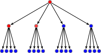
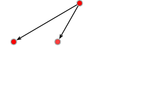
Figure 2: (a) For a fixed η>0\eta>0, the red nodes have the refinement quantity above η\eta: δj,k(f)>η\delta_{j,k}(f)>\eta. The master tree is then truncated to the smallest subtree containing the red nodes in (b). In (c), the outer leaves of the truncated tree are given by the green nodes. The corresponding adaptive partition is given in (d).

In the tree-based nonlinear approximation, one fixes a threshold value η>0\eta>0, and truncate 𝒯\mathcal{T} to 𝒯(f,η)\mathcal{T}(f,\eta) – the smallest subtree that contains all Cj,k𝒟C_{j,k}\in\mathcal{D} with δj,k(f)>η\delta_{j,k}(f)>\eta. The collection of outer leaves of 𝒯(f,η)\mathcal{T}(f,\eta), denoted by Λ(f,η)\Lambda(f,\eta), gives rise to an adaptive partition. This truncation procedure is illustrated in Figure 2. In Figure 2, the red nodes have the refinement quantity above η\eta, and then the master tree 𝒯\mathcal{T} is truncated to the smallest subtree containing the red nodes in (b). The outer leaves of this truncated tree are given by the green nodes in Figure 2 (c), and the corresponding adaptive partition is given in Figure 2 (d).

The piecewise polynomial approximation of ff on this adaptive partition is

pΛ(f,η)=Cj,kΛ(f,η)pj,k(f)χCj,k.\displaystyle p_{\Lambda(f,\eta)}=\sum_{C_{j,k}\in\Lambda(f,\eta)}p_{j,k}(f)\chi_{C_{j,k}}. (7)

In the adaptive approximation, the regularity of ff can be defined by the size of the tree #𝒯(f,η)\#\mathcal{T}(f,\eta).

Definition 3 ((2.19) in Binev et al. (2007)).

For a fixed s>0s>0, a polynomial degree θ\theta, we let the function class 𝒜θs\mathcal{A}^{s}_{\theta} be the collection of all fL2(X)f\in L^{2}(X), such that

|f|𝒜θsm=supη>0ηm#𝒯(f,η)<,with m=22s+1,|f|_{\mathcal{A}^{s}_{\theta}}^{m}=\sup_{\eta>0}\eta^{m}\#\mathcal{T}(f,\eta)<\infty,\quad\text{with }\ m=\frac{2}{2s+1}, (8)

where 𝒯(f,η)\mathcal{T}(f,\eta) is the truncated tree of approximating ff with piecewise θ\theta-th order polynomials with threshold η\eta.

In Definition 3, the complexity of the adaptive approximation is measured by the cardinality of the truncated tree 𝒯(f,η)\mathcal{T}(f,\eta). In fact, the cardinality of the adaptive partition Λ(f,η)\Lambda(f,\eta) is related with the cardinality of the truncated tree 𝒯(f,η)\mathcal{T}(f,\eta) such that

#𝒯(f,η)#Λ(f,η)2d#𝒯(f,η).\#\mathcal{T}(f,\eta)\leq\#\Lambda(f,\eta)\leq 2^{d}\#\mathcal{T}(f,\eta). (9)

The lower bound follows from

#𝒯(f,η)\displaystyle\#\mathcal{T}(f,\eta) k=1#Λ(f,η)(2d)k=#Λ(f,η)2d(112d)#Λ(f,η).\displaystyle\leq\sum_{k=1}^{\infty}\frac{\#\Lambda(f,\eta)}{(2^{d})^{k}}=\frac{\#\Lambda(f,\eta)}{2^{d}(1-\frac{1}{2^{d}})}\leq\#\Lambda(f,\eta).

The definition of 𝒜θs\mathcal{A}^{s}_{\theta} does not explicitly depend on the dimension dd. The dimension dd is actually hidden in the regularity parameter ss (see Example 1a). This way of definition has the advantage of adapting to low-dimensional structures in the data distribution (see Example 5a).

When f𝒜θsf\in\mathcal{A}^{s}_{\theta}, we have the approximation error

fpΛ(f,η)L2(ρ)2Cs|f|𝒜θsmη2mCs|f|𝒜θs2(#𝒯(f,η))2s,\|f-p_{\Lambda(f,\eta)}\|_{L^{2}(\rho)}^{2}\leq C_{s}|f|_{\mathcal{A}^{s}_{\theta}}^{m}\eta^{2-m}\leq C_{s}|f|_{\mathcal{A}^{s}_{\theta}}^{2}(\#\mathcal{T}(f,\eta))^{-{2s}}, (10)

where

Cs=2m02(m2),with m=22s+1.C_{s}=2^{m}\sum_{\ell\geq 0}2^{\ell(m-2)},\quad\text{with }\ m=\frac{2}{2s+1}. (11)

The approximation error in (10) is proved in Appendix A. The original proof can be found in Binev et al. (2007, 2005); Cohen et al. (2001).

3.2 Case Study of the 𝒜θs\mathcal{A}^{s}_{\theta} Function Class

The 𝒜θs\mathcal{A}^{s}_{\theta} class contains a large collection of functions, including Hölder functions, piecewise Hölder functions, functions which are irregular on a set of measure zero, and regular functions with distribution concentrated on a low-dimensional manifold. For some examples to be studied below, we make the following assumption on the measure ρ\rho:

Assumption 1.

There exists a constant Cρ>0C_{\rho}>0 such that any subset SXS\subset X satisfies

ρ(S)Cρ|S|,\rho(S)\leq C_{\rho}|S|,

where |S||S| is the Lebesgue measure of SS.

3.2.1 Hölder functions

Example 1a (Hölder functions).

Let r>0r>0. Under Assumption 1, the rr-Hölder function class r(X)\mathcal{H}^{r}(X) belongs to 𝒜r1r/d\mathcal{A}^{r/d}_{\lceil r-1\rceil}. If fr(X)f\in\mathcal{H}^{r}(X), then we have f𝒜r1r/df\in\mathcal{A}^{r/d}_{\lceil r-1\rceil}. Furthermore, if fr(X)1\|f\|_{\mathcal{H}^{r}(X)}\leq 1, then

|f|𝒜r1r/dC(r,d,Cρ)|f|_{\mathcal{A}^{r/d}_{\lceil r-1\rceil}}\leq C(r,d,C_{\rho}) (12)

for some constant C(r,d,Cρ)C(r,d,C_{\rho}) depending on r,dr,d and CρC_{\rho} in Assumption 1.

Example 1a is proved in Section 6.4.1. At the end of Example 1a, we assume fr(X)1\|f\|_{\mathcal{H}^{r}(X)}\leq 1 without loss of generality. The same statement holds if fr(X)\|f\|_{\mathcal{H}^{r}(X)} is bounded by an absolute constant. Such a constant only changes the ||𝒜r1r/d|\cdot|_{\mathcal{A}^{r/d}_{\lceil r-1\rceil}} bound in (12), i.e. C(r,d,Cρ)C(r,d,C_{\rho}) will depends on this constant.

The neural network approximation theory for Hölder functions is given in Example 1b and the generalization theory is given in Example 1c.
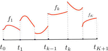
Refer to caption
(a) 1D piecewise Hölder function
Refer to caption
(b) 2D piecewise domain
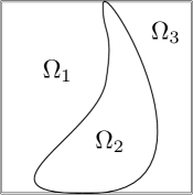
Figure 3: (a) Example 2a: 1D piecewise Hölder function with KK discontinuity points; (b) Example 3a: A 2D piecewise domain. The functions in Example 3a are rr-Hölder in the interior of Ω1,Ω2,Ω3\Omega_{1},\Omega_{2},\Omega_{3}.

3.2.2 Piecewise Hölder functions in 1D

Example 2a (Piecewise Hölder functions in 1D).

Let d=1d=1, r>0r>0 and KK be a positive integer. Under Assumption 1, all bounded piecewise rr-Hölder functions with KK discontinuity points belong to f𝒜r1rf\in\mathcal{A}^{r}_{\lceil r-1\rceil}. Specifically, let ff be a piecewise rr-Hölder function such that f=k=1K+1fkχ[tk1,tk)f=\sum_{k=1}^{K+1}f_{k}\chi_{[t_{k-1},t_{k})}, where 0=t0<t1<<tK<tK+1=10=t_{0}<t_{1}<\ldots<t_{K}<t_{K+1}=1. Each function fk:[tk1,tk)f_{k}:[t_{k-1},t_{k})\rightarrow\mathbb{R} is rr-Hölder in (tk1,tk)(t_{k-1},t_{k}), and ff is discontinuous at t1,t2,tKt_{1},t_{2},\ldots t_{K}. Assume ff is bounded such that fL([0,1])1\|f\|_{L^{\infty}([0,1])}\leq 1. In this case, we have f𝒜r1rf\in\mathcal{A}^{r}_{\lceil r-1\rceil}. See Figure 3 (a) for an illustration of a piecewise Hölder function in 1D. Furthermore, if maxkfr(tk,tk+1)1,\max_{k}\|f\|_{\mathcal{H}^{r}(t_{k},t_{k+1})}\leq 1, then

|f|𝒜r1rC(r,d,Cρ,K)|f|_{\mathcal{A}^{r}_{\lceil r-1\rceil}}\leq C(r,d,C_{\rho},K)

for some constant C(r,d,Cρ,K)C(r,d,C_{\rho},K) depending on r,d,Kr,d,K and CρC_{\rho} in Assumption 1, and does not depend on specific tkt_{k}’s.

Example 2a is proved in Section 6.4.2. Example 2a demonstrates that, for 1D bounded piecewise rr-Hölder functions with a finite number of discontinuities, the overall regularity index is s=rs=r under Definition 3. In comparison with Example 1a, we prove that, a finite number of discontinuities in 1D does not affect the regularity index in Definition 3.

The neural network approximation theory for piecewise Hölder functions in 1D is given in Example 2b and the generalization theory is given in Example 2c.

3.2.3 Piecewise Hölder functions in multi-dimensions

In the next example, we will see that, for piecewise rr-Hölder functions in multi-dimensions, the overall approximation error is dominated either by the approximation error in the interior of each piece or by the error along the discontinuity. The overall regularity index ss depends on rr and dd.

Example 3a (Piecewise Hölder functions in multi-dimensions).

Let d2d\geq 2, r>0r>0 and {Ωt}t=1T\{\Omega_{t}\}_{t=1}^{T} be subsets of [0,1]d[0,1]^{d} such that t=1TΩt=[0,1]d\cup_{t=1}^{T}\Omega_{t}=[0,1]^{d} and the Ωt\Omega_{t}’s only overlap at their boundaries. Each Ωt\Omega_{t} is a connected subset of [0,1]d[0,1]^{d} and the union of their boundaries tΩt\cup_{t}\partial\Omega_{t} has upper Minkowski dimension d1d-1. See Figure 3 (b) for an illustration of the Ωt\Omega_{t}’s. When ρ\rho satisfies Assumption 1, all piecewise rr-Hölder functions with discontinuity on tΩt\cup_{t}\partial\Omega_{t} belong to

𝒜r1s,wheres=min{rd,12(d1)}.\mathcal{A}^{s}_{\lceil r-1\rceil},\ \text{where}\ s=\min\left\{\frac{r}{d},\frac{1}{2(d-1)}\right\}. (13)

Specifically, let ff be a piecewise rr-Hölder function such that f=t=1TftχΩtf=\sum_{t=1}^{T}f_{t}\chi_{\Omega_{t}} where χΩt\chi_{\Omega_{t}} is the indicator function on Ωt\Omega_{t}. Each function ft:Ωtf_{t}:\Omega_{t}\rightarrow\mathbb{R} is rr-Hölder in the interior of Ωt\Omega_{t}: ftr(Ωto)f_{t}\in\mathcal{H}^{r}(\Omega_{t}^{o}) where Ωto\Omega_{t}^{o} denotes the interior of Ωt\Omega_{t}, and ff is discontinuous at tΩt\cup_{t}\partial\Omega_{t}. Assume ff is bounded such that fL([0,1]d)1\|f\|_{L^{\infty}([0,1]^{d})}\leq 1. In this case, f𝒜r1sf\in\mathcal{A}^{s}_{\lceil r-1\rceil} with the ss given in (13). Furthermore, if maxtfr(Ωto)1\max_{t}\|f\|_{\mathcal{H}^{r}(\Omega_{t}^{o})}\leq 1, then

|f|𝒜r1sC(r,d,cM(tΩt),Cρ)|f|_{\mathcal{A}^{s}_{\lceil r-1\rceil}}\leq C(r,d,c_{M}(\cup_{t}\partial\Omega_{t}),C_{\rho})

for some C(r,d,cM(tΩt),Cρ)C(r,d,c_{M}(\cup_{t}\partial\Omega_{t}),C_{\rho}) depending on r,d,cM(tΩt)r,d,c_{M}(\cup_{t}\partial\Omega_{t}) (the Minkowski dimension constant of tΩt\cup_{t}\partial\Omega_{t} defined in Definition 2) and CρC_{\rho} in Assumption 1.

Example 3a is proved in Section 6.4.3. Example 3a demonstrates that, for piecewise rr-Hölder functions with discontinuity on a subset with upper Minkowski dimension d1d-1, the overall regularity index ss has a phase transition. When rd12(d1)\frac{r}{d}\leq\frac{1}{2(d-1)}, the approximation error is dominated by that in the interior of the Ωt\Omega_{t}’s. When rd>12(d1)\frac{r}{d}>\frac{1}{2(d-1)}, the approximation error is dominated by that around the boundary of the Ωt\Omega_{t}’s. As the result, the overall regularity index ss is the minimum of rd\frac{r}{d} and 12(d1)\frac{1}{2(d-1)}.

The neural network approximation theory for piecewise Hölder functions in multi-dimensions is given in Example 3b and the generalization theory is given in Example 3c.

3.2.4 Functions irregular on a set of measure zero

The definition of 𝒜θs\mathcal{A}^{s}_{\theta} is dependent on the measure ρ\rho, since the refinement quantity δj,k\delta_{j,k} is the L2L^{2} norm with respect to ρ\rho. This measure-dependent definition is not only adaptive to the regularity of ff, but also adaptive to the distribution ρ\rho. In the following example, we show that, the definition of 𝒜θs\mathcal{A}^{s}_{\theta} allows the function ff to be irregular on a set of measure zero. For δ>0\delta>0, Ωδ\Omega_{\delta} denotes the set within δ\delta distance to Ω\Omega such that Ωδ={xX:dist(x,Ω)=infzΩxzδ}\Omega_{\delta}=\{x\in X:\ {\rm dist}(x,\Omega)=\inf_{z\in\Omega}\|x-z\|\leq\delta\}.

Example 4a (Functions irregular on a set of measure zero).

Let δ>0\delta>0, Ω\Omega be a subset of X=[0,1]dX=[0,1]^{d} and Ω=XΩ\Omega^{\complement}=X\setminus\Omega. If ff is an rr-Hölder function on Ωδ\Omega_{\delta} and ρ(Ω)=0\rho(\Omega^{\complement})=0, then f𝒜r1r/df\in\mathcal{A}^{r/d}_{\lceil r-1\rceil}. Furthermore, if fr(Ωδ)1\|f\|_{\mathcal{H}^{r}(\Omega_{\delta})}\leq 1, then

|f|𝒜r1r/dC(r,d,Cρ)|f|_{\mathcal{A}^{r/d}_{\lceil r-1\rceil}}\leq C(r,d,C_{\rho})

for some constant C(r,d,Cρ)C(r,d,C_{\rho}) depending on r,dr,d and CρC_{\rho} in Assumption 1.

Example 4a is proved in Section 6.4.4. In Example 4a, ff is rr-Hölder on Ωδ\Omega_{\delta}, and can be irregular on a measure zero set. In comparison with Example 1a, such irregularity on a set of measure zero does not affect the smoothness parameter in Definition 3. In this example, we set Ωδ\Omega_{\delta} to be a larger set than Ω\Omega, in order to avoid the discontinuity effect at the boundary of Ω\Omega.

The neural network approximation theory for functions in Example 4a is given in Example 4b and the generalization theory is given in Example 4c.

3.2.5 Hölder functions with distribution concentrated on a low-dimensional manifold

Since the definition of 𝒜θs\mathcal{A}^{s}_{\theta} is dependent on the probability measure ρ\rho, this definition is also adaptive to lower-dimensional sets in XX. We next consider a probability measure ρ\rho concentrated on a dind_{\rm in}-dimensional manifold isometrically embedded in XX.

Example 5a (Hölder functions with distribution concentrated on a low-dimensional manifold).

Let r>0r>0. Suppose X=[0,1]dX=[0,1]^{d} can be decomposed to Ω\Omega and Ω\Omega^{\complement}, i.e. X=ΩΩX=\Omega\cup\Omega^{\complement} where Ω\Omega is a compact dind_{\rm in}-dimensional Riemannian manifold isometrically embedded in XX. Assume that ρ(Ω)=0\rho(\Omega^{\complement})=0, and ρ\rho conditioned on Ω\Omega is the uniform distribution on Ω\Omega. If fr(X)f\in\mathcal{H}^{r}(X), then f𝒜r1r/dinf\in\mathcal{A}^{r/{d_{\rm in}}}_{\lceil r-1\rceil}. Furthermore, if fr(X)1\|f\|_{\mathcal{H}^{r}(X)}\leq 1, then

|f|𝒜r1r/din<C(r,d,din,τ,|Ω|)|f|_{\mathcal{A}^{r/d_{\rm in}}_{\lceil r-1\rceil}}<C(r,d,d_{\rm in},\tau,|\Omega|)

with C(r,d,din,τ,|Ω|)C(r,d,d_{\rm in},\tau,|\Omega|) depending on r,d,din,τr,d,d_{\rm in},\tau and |Ω||\Omega|, where τ\tau is the reach (Federer, 1959) of Ω\Omega and |Ω||\Omega| is the surface area of Ω\Omega.

Example 5a is proved in Section 6.4.5. In this example, the function ff is rr-Hölder on XX, but the measure ρ\rho is supported on a lower dimensional manifold with intrinsic dimension dind_{\rm in}. The regularity index under Definition 3 is r/dinr/{d_{\rm in}} instead of r/dr/d.

4 Adaptive approximation and generalization theory of deep neural networks

This section contains our main results: approximation and generalization theories of deep ReLU networks for the 𝒜θs\mathcal{A}^{s}_{\theta} function class. We present some preliminaries in Subsection 4.1, the approximation theory in Subsection 4.2, case studies of the approximation error in Subsection 4.3, the generalization theory in Subsection 4.4, and case studies of the generalization error in Subsection 4.5.

4.1 Preliminaries

Each Cj,kC_{j,k} is a hypercube in the form of =1d[r,j,k,r,j,k+2j]\otimes_{\ell=1}^{d}[r_{\ell,j,k},r_{\ell,j,k}+2^{-j}], where r,j,k[0,1]r_{\ell,j,k}\in[0,1] is a scalar and

=1d[r,j,k,r,j,k+2j]=[r1,j,k,r1,j,k+2j]××[rd,j,k,rd,j,k+2j]\displaystyle\otimes_{\ell=1}^{d}[r_{\ell,j,k},r_{\ell,j,k}+2^{-j}]=[r_{1,j,k},r_{1,j,k}+2^{-j}]\times\cdots\times[r_{d,j,k},r_{d,j,k}+2^{-j}] (14)

is a hypercube with edge length 2j2^{-j} in d\mathbb{R}^{d}.

The collection of polynomials ((𝐱𝐫j,k)/2j)𝜶\left((\mathbf{x}-\mathbf{r}_{j,k})/{2^{-j}}\right)^{\bm{\alpha}} form a basis for the space of dd-variable polynomials of degree no more than θ\theta. Let ρ\rho be a measure on [0,1]d[0,1]^{d} and fL2(ρ)f\in L^{2}(\rho). The piecewise polynomial approximator pj,kp_{j,k} for ff can be written as

pj,k(𝐱)=|𝜶|θa𝜶(𝐱𝐫j,k2j)𝜶,\displaystyle p_{j,k}(\mathbf{x})=\sum_{|\bm{\alpha}|\leq\theta}a_{\bm{\alpha}}\left(\frac{\mathbf{x}-\mathbf{r}_{j,k}}{2^{-j}}\right)^{\bm{\alpha}}, (15)

where 𝐫j,k=[r1,j,k,,rd,j,k]\mathbf{r}_{j,k}=[r_{1,j,k},...,r_{d,j,k}].

In this paper, we focus on the set of functions with bounded coefficients in the piecewise polynomial approximation.

Assumption 2.

Let s,R𝒜,R,Rp>0s,R_{\mathcal{A}},R,R_{p}>0, θ\theta be a nonnegative integer, and ρ\rho be a probability measure on [0,1]d[0,1]^{d}. We assume f𝒜θsf\in\mathcal{A}^{s}_{\theta} and

  • (i)

    |f|𝒜θsR𝒜|f|_{\mathcal{A}^{s}_{\theta}}\leq R_{\mathcal{A}},

  • (ii)

    fL([0,1]d)R\|f\|_{L^{\infty}([0,1]^{d})}\leq R,

  • (iii)

    On every Cj,kC_{j,k}, the polynomial approximator pj,kp_{j,k} for ff in the form of (15) satisfies |a𝜶|Rp|a_{\bm{\alpha}}|\leq R_{p} for all 𝜶\bm{\alpha} with |𝜶|θ|\bm{\alpha}|\leq\theta.

By Assumption 2 (i) and (ii), ff has a bounded ||𝒜θs|\cdot|_{\mathcal{A}^{s}_{\theta}} quantity and LL^{\infty} norm, which is a common assumption in nonparametric estimation theory (Györfi et al., 2002). Assumption 2 (iii) requires the polynomial coefficients in the best polynomial approximating ff on every Cj,kC_{j,k} to be uniformly bounded by RpR_{p}. The following lemma shows that Assumption 2 (iii) can be implied from Assumption 2 (ii) when ρ\rho is the Lebesgue measure on X=[0,1]dX=[0,1]^{d}.

Lemma 1.

Let R>0R>0, θ\theta be a fixed nonnegative integer, and ρ\rho be the Lebesgue measure on X=[0,1]dX=[0,1]^{d}. There exists a constant Rp>0R_{p}>0 depending on θ,d\theta,d and RR such that, for any function ff on [0,1]d[0,1]^{d} satisfying fL(X)R\|f\|_{L^{\infty}(X)}\leq R, the pj,kp_{j,k} in (4) has the form of (15) with |a𝜶|Rp,𝜶|a_{\bm{\alpha}}|\leq R_{p},\ \forall\bm{\alpha} with |𝜶|θ|\bm{\alpha}|\leq\theta and pj,kL(Cj,k)CRp\|p_{j,k}\|_{L^{\infty}(C_{j,k})}\leq CR_{p} for some CC depending on dd and θ\theta.

Lemma 1 is proved in Appendix B. Lemma 1 implies that under the Lebesgue measure, for any pj,kp_{j,k} in the form of (15), the coefficients a𝜶a_{\bm{\alpha}}’s are uniformly bounded by a constant depending on θ,d,R\theta,d,R, and is independent to the index (j,k)(j,k). Thus Assumption 2(iii) holds.

4.2 Approximation Theory

Our approximation theory shows that deep neural networks give rise to universal approximations for functions in the 𝒜θs\mathcal{A}^{s}_{\theta} class under Assumption 2 if the network architecture is properly chosen.

Theorem 1 (Approximation).

Let s,d,Cρ,R𝒜,R,Rp>0s,d,C_{\rho},R_{\mathcal{A}},R,R_{p}>0 and θ\theta be a nonnegative integer. For any ε>0\varepsilon>0, there is a ReLU network class =NN(L,w,K,κ,M)\mathcal{F}=\mathcal{F}_{\rm NN}(L,w,K,\kappa,M) with parameters

L=O(log1ε),w=O(ε1s),K=O(ε1slog1ε),κ=O(εmax{2,1s}),M=R,\displaystyle L=O\left(\log\frac{1}{\varepsilon}\right),\ w=O(\varepsilon^{-\frac{1}{s}}),\ K=O\left(\varepsilon^{-\frac{1}{s}}\log\frac{1}{\varepsilon}\right),\ \kappa=O(\varepsilon^{-\max\{2,\frac{1}{s}\}}),\ M=R, (16)

such that, for any ρ\rho satisfying Assumption 1 and any f𝒜θsf\in\mathcal{A}^{s}_{\theta} satisfying Assumption 2, if the weight parameters of the network are properly chosen, the network yields a function f~\widetilde{f}\in\mathcal{F} such that

f~fL2(ρ)2ε.\displaystyle\|\widetilde{f}-f\|_{L^{2}(\rho)}^{2}\leq\varepsilon. (17)

The constants hidden in O()O(\cdot) depends on dd (the dimension of the domain for ff), CρC_{\rho} (in Assumption 1), θ\theta (the polynomial order), ss, RR, RpR_{p} and R𝒜R_{\mathcal{A}} (in Assumption 2).

Theorem 1 is proved in Section 6.2. Theorem 1 demonstrates the universal approximation power of deep neural networks for the 𝒜θs\mathcal{A}^{s}_{\theta} function class. The parameters in (16) specifies the network architecture. To approximate a specific function f𝒜θsf\in\mathcal{A}^{s}_{\theta}, there exist some proper weight parameters which give rise to a network function f~\widetilde{f} to approximate ff.

4.3 Case Studies of the Approximation Error

In this subsection, we apply Theorem 1 to the examples in Subsection 3.2, and derive the approximation theory for each example. In the following case studies, we need Assumptions 1, 2 (iii) and 3, but not Assumption 2 (i) - (ii). In each case, we have shown in Subsection 3.2 that Assumption 2 (i) holds: f𝒜θsf\in\mathcal{A}^{s}_{\theta} with a proper θ\theta and the regularity index ss depends on each specific case.

4.3.1 Hölder functions

Consider Hölder functions in Example 1a such that r𝒜r1r/d\mathcal{H}^{r}\subset\mathcal{A}^{r/d}_{\lceil r-1\rceil}. Applying Theorem 1 gives rise to the following neural network approximation theory for Hölder functions.

Example 1b (Hölder functions).

Let r,d,Cρ,Rp>0r,d,C_{\rho},R_{p}>0. For any ε>0\varepsilon>0, there is a ReLU network class =NN(L,w,K,κ,M)\mathcal{F}=\mathcal{F}_{\rm NN}(L,w,K,\kappa,M) with parameters

L=O(log1ε),w=O(εdr),K=O(εdrlog1ε),κ=O(εmax{2,dr}),M=1,\displaystyle L=O\left(\log\frac{1}{\varepsilon}\right),\ w=O(\varepsilon^{-\frac{d}{r}}),\ K=O\left(\varepsilon^{-\frac{d}{r}}\log\frac{1}{\varepsilon}\right),\ \kappa=O(\varepsilon^{-\max\{2,\frac{d}{r}\}}),\ M=1,

such that for any ρ\rho satisfying Assumption 1 and any function fr(X)f\in\mathcal{H}^{r}(X) satisfying fr(X)1\|f\|_{\mathcal{H}^{r}(X)}\leq 1 and Assumption 2 (iii), if the weight parameters of the network are properly chosen, the network yields a function f~\widetilde{f}\in\mathcal{F} such that

f~fL2(ρ)2ε.\displaystyle\|\widetilde{f}-f\|_{L^{2}(\rho)}^{2}\leq\varepsilon.

The constant hidden in O()O(\cdot) depends on r,d,Cρ,Rpr,d,C_{\rho},R_{p}.

Example 1b is a corollary of Theorem 1 with s=r/ds=r/d. Note that Assumption 2(i) and (ii) are implied by the condition fr(X)1\|f\|_{\mathcal{H}^{r}(X)}\leq 1. In particular, fr(X)1\|f\|_{\mathcal{H}^{r}(X)}\leq 1 implies fL(X)1\|f\|_{L^{\infty}(X)}\leq 1 according to (1). Furthermore, If fr(X)1\|f\|_{\mathcal{H}^{r}(X)}\leq 1, then |f|𝒜r1r/dC(r,d,Cρ)|f|_{\mathcal{A}^{r/d}_{\lceil r-1\rceil}}\leq C(r,d,C_{\rho}) according to our argument in Example 1a.

In litertuare, the approximation theory of ReLU networks for Sobolev functions in Wr,W^{r,\infty} has been established in Yarotsky (2017, Theorem 1). The proof in Yarotsky (2017, Theorem 1) can be applied to Hölder functions. Our network size in Example 1b is comparable to that in Yarotsky (2017, Theorem 1).

4.3.2 Piecewise Hölder functions in 1D

Considering 1D piecewise Hölder functions in Example 2a, we have the following approximation theory:

Example 2b (Piecewise Hölder functions in 1D).

Let r,Cρ,Rp,K>0r,C_{\rho},R_{p},K>0. For any ε>0\varepsilon>0, there is a ReLU network class =NN(L,w,K,κ,M)\mathcal{F}=\mathcal{F}_{\rm NN}(L,w,K,\kappa,M) with parameters

L=O(log1ε),w=O(ε1r),K=O(ε1rlog1ε),κ=O(εmax{2,1r}),M=1,\displaystyle L=O\left(\log\frac{1}{\varepsilon}\right),\ w=O(\varepsilon^{-\frac{1}{r}}),\ K=O\left(\varepsilon^{-\frac{1}{r}}\log\frac{1}{\varepsilon}\right),\ \kappa=O(\varepsilon^{-\max\{2,\frac{1}{r}\}}),\ M=1, (18)

such that for any ρ\rho satisfing Assumption 1, and any piecewise rr-Hölder function in the form of f=k=1K+1fkχ[tk1,tk)f=\sum_{k=1}^{K+1}f_{k}\chi_{[t_{k-1},t_{k})} in Example 2a satisfying fL([0,1])1\|f\|_{L^{\infty}([0,1])}\leq 1, maxkfkr(tk,tk+1)1\max_{k}\|f_{k}\|_{\mathcal{H}^{r}(t_{k},t_{k+1})}\leq 1 and Assumption 2(iii), if the weight parameters of the network are properly chosen, the network yields a function f~\widetilde{f}\in\mathcal{F} such that

f~fL2(ρ)2ε.\displaystyle\|\widetilde{f}-f\|_{L^{2}(\rho)}^{2}\leq\varepsilon.

The constant hidden in O()O(\cdot) depends on r,Cρ,Rp,Kr,C_{\rho},R_{p},K.

Example 2b is a corollary of Theorem 1 with f𝒜r1rf\in\mathcal{A}^{r}_{\lceil r-1\rceil}. Assumption 2 (i) is not explicitly enforced in Example 2b , but is implied from the condition of maxkfkr(tk,tk+1)1\max_{k}\|f_{k}\|_{\mathcal{H}^{r}(t_{k},t_{k+1})}\leq 1 by Example 2a. Example 2b shows that, to achieve an ε\varepsilon approximation error for 1D functions with a finite number of discontinuities, the network size is comparable to that for 1D Hölder functions in Example 1b.

4.3.3 Piecewise Hölder function in multi-dimensions

Considering piecewise Hölder functions in multi-dimensions in Example 3a, we have the following approximation theory:

Example 3b (Piecewise Hölder functions in multi-dimensions).

Let d2d\geq 2, r,Cρ,Rp,T>0r,C_{\rho},R_{p},T>0 and {Ωt}t=1T\{\Omega_{t}\}_{t=1}^{T} be subsets of [0,1]d[0,1]^{d} such that t=1TΩt=[0,1]d\cup_{t=1}^{T}\Omega_{t}=[0,1]^{d} and the Ωt\Omega_{t}’s only overlap at their boundaries. Each Ωt\Omega_{t} is a connected subset of [0,1]d[0,1]^{d} and the union of their boundaries t=1TΩt\cup_{t=1}^{T}\partial\Omega_{t} has upper Minkowski dimension d1d-1. Denote the Minkowski dimension constant of t=1TΩt\cup_{t=1}^{T}\partial\Omega_{t} by cM(tΩt)c_{M}(\cup_{t}\partial\Omega_{t}). For any ε>0\varepsilon>0, there is a ReLU network class =NN(L,w,K,κ,M)\mathcal{F}=\mathcal{F}_{\rm NN}(L,w,K,\kappa,M) with parameters

L=O(log1ε),w=O(εmax{dr,2(d1)}),K=O(εmax{dr,2(d1)}log1ε),\displaystyle L=O\left(\log\frac{1}{\varepsilon}\right),\ w=O(\varepsilon^{-\max\left\{\frac{d}{r},2(d-1)\right\}}),\ K=O\left(\varepsilon^{-\max\left\{\frac{d}{r},2(d-1)\right\}}\log\frac{1}{\varepsilon}\right),
κ=O(εmax{2,dr,2(d1)}),M=1,\displaystyle\kappa=O(\varepsilon^{-\max\{2,\frac{d}{r},2(d-1)\}}),\ M=1,

such that for any ρ\rho satisfying Assumption 1, and any piecewise rr-Hölder function in the form of f=t=1TftχΩtf=\sum_{t=1}^{T}f_{t}\chi_{\Omega_{t}} in Example 3a satisfying fL([0,1]d)1\|f\|_{L^{\infty}([0,1]^{d})}\leq 1, maxtftr(Ωto)1\max_{t}\|f_{t}\|_{\mathcal{H}^{r}(\Omega_{t}^{o})}\leq 1 and Assumption 2(iii), if the weight parameters of the network are properly chosen, the network yields a function f~\widetilde{f}\in\mathcal{F} such that

f~fL2(ρ)2ε.\displaystyle\|\widetilde{f}-f\|_{L^{2}(\rho)}^{2}\leq\varepsilon.

The constant hidden in O()O(\cdot) depends on r,d,cM(tΩt),Cρ,Rpr,d,c_{M}(\cup_{t}\partial\Omega_{t}),C_{\rho},R_{p}.

Example 3b is a corollary of Theorem 1 with f𝒜r1sf\in\mathcal{A}^{s}_{\lceil r-1\rceil} for the ss given in (13). Assumption 2 (i) is not explicitly enforced in Example 3b , but is implied from the condition of maxkfkr(tk,tk+1)1\max_{k}\|f_{k}\|_{\mathcal{H}^{r}(t_{k},t_{k+1})}\leq 1 by Example 3a. Example 3b implies that to approximate a piecewise Hölder function in Example 3a, the number of nonzero weight parameters is in the order of εmax{dr,2(d1)}log1ε\varepsilon^{-\max\left\{\frac{d}{r},2(d-1)\right\}}\log\frac{1}{\varepsilon}. The discontinuity set in Example 3b has upper Minkowski dimension d1d-1, which is a weak assumption without additional regularity assumption or low-dimensional structures.

Neural network approximation theory for piecewise smooth functions has been considered in Petersen and Voigtlaender (2018). The setting in Petersen and Voigtlaender (2018) is similar but different from that of Example 3b. In Petersen and Voigtlaender (2018), the authors considered piecewise functions f:[1/2,1/2]df:[-1/2,1/2]^{d}\rightarrow\mathbb{R}, where the different “smooth regions” of ff are separated by β\mathcal{H}^{\beta} hypersurfaces. If ff is a piecewise rr-Hölder function and the Hölder norm of ff on each piece is bounded, it is shown in Petersen and Voigtlaender (2018, Corollary 3.7) that such ff can be universally approximated by a ReLU network with at most cεp(d1)/βc\varepsilon^{-p(d-1)/\beta} weight parameters to guarantee an LpL^{p} approximation error ε\varepsilon. It is further shown in Petersen and Voigtlaender (2018, Theorem 4.2) that, to achieve an LpL^{p} approximation error ε\varepsilon, the optimal required number of weight parameters is lower bounded in the order of εp(d1)/β/log1ε\varepsilon^{-{p(d-1)}/{\beta}}/\log\frac{1}{\varepsilon}. Our result in Example 3b is comparable to that of Petersen and Voigtlaender (2018) when β=1\beta=1 and p=2p=2. When the discontinuity hypersurface has higher order regularity, i.e. β>1\beta>1, the network size in Petersen and Voigtlaender (2018) is smaller/better than that in Example 3b since the higher order smoothness of the discontinuity hypersurface is exploited in the approximation theory. However, Example 3b imposes a weaker assumption on the discontinuity hypersurface. Example 3b requires the discontinuity hypersurface to have upper Minkowski dimension d1d-1, while the the discontinuity hypersurface in Petersen and Voigtlaender (2018, Definition 3.3) is the graph of a β\mathcal{H}^{\beta} function on d1d-1 coordinates. In this sense, Example 3b can be applied to a wider class of piecewise Hölder functions.

4.3.4 Functions irregular on a set of measure zero

Functions in the 𝒜θs\mathcal{A}^{s}_{\theta} class can be irregular on a set of measure zero, as in Example 4a. The approximation theory for functions in Example 4a is given below:

Example 4b (Functions irregular on a set of measure zero).

Let r,d,Cρ,Rp,δ>0r,d,C_{\rho},R_{p},\delta>0 and Ω\Omega be a subset of XX. For any ε>0\varepsilon>0, there is a ReLU network class =NN(L,w,K,κ,M)\mathcal{F}=\mathcal{F}_{\rm NN}(L,w,K,\kappa,M) with parameters

L=O(log1ε),w=O(εdr),K=O(εdrlog1ε),κ=O(εmax{2,dr}),M=1.\displaystyle L=O\left(\log\frac{1}{\varepsilon}\right),\ w=O(\varepsilon^{-\frac{d}{r}}),\ K=O\left(\varepsilon^{-\frac{d}{r}}\log\frac{1}{\varepsilon}\right),\ \kappa=O(\varepsilon^{-\max\{2,\frac{d}{r}\}}),\ M=1.

For any ρ\rho satisfying Assumption 1 and ρ(Ω)=0\rho(\Omega^{\complement})=0, and for any f:Xf:X\rightarrow\mathbb{R} satisfying fr(Ωδ)1\|f\|_{\mathcal{H}^{r}(\Omega_{\delta})}\leq 1 and Assumption 2(iii), if the weight parameters of the network are properly chosen, the network class yields a function f~\widetilde{f}\in\mathcal{F} such that

f~fL2(ρ)2ε.\displaystyle\|\widetilde{f}-f\|_{L^{2}(\rho)}^{2}\leq\varepsilon.

The constant hidden in O()O(\cdot) depends on r,d,Cρ,Rpr,d,C_{\rho},R_{p}.

Example 4b is a corollary of Theorem 1 with f𝒜r1r/df\in\mathcal{A}^{r/d}_{\lceil r-1\rceil} and |f|𝒜r1r/dC(r,d,Cρ)|f|_{\mathcal{A}^{r/d}_{\lceil r-1\rceil}}\leq C(r,d,C_{\rho}) by Example 4a. Example 4b shows that function irregularity on a set of measure zero does not affect the network size in approximation theory.

4.3.5 Hölder functions with distribution concentrated on a low-dimensional manifold

Theorem 1 cannot be directly applied to Example 5a, since Assumption 1 is violated when ρ\rho is supported on a low-dimensional manifold. In literature, neural network approximation theory has been established in Chen et al. (2019a) for functions on a low-dimensional manifold, and in Nakada and Imaizumi (2020) for Hölder functions in [0,1]D[0,1]^{D} while the support of measure has a low Minkowski dimension. See Section 4.5.5 for a detailed discussion about the generalization error.

4.4 Generalization Error

Theorem 1 proves the existence of a neural network f~\widetilde{f} to approximate ff with an arbitrary accuracy ε\varepsilon, but it does not give an explicit method to find the weight parameters of f~\widetilde{f}. In practice, the weight parameters are learned from data through the empirical risk minimization. The generalization error of the empirical risk minimizer is analyzed in this subsection.

Suppose the training data set is 𝒮={𝐱i,yi}i=1n{\mathcal{S}}=\{\mathbf{x}_{i},y_{i}\}_{i=1}^{n} where the 𝐱i\mathbf{x}_{i}’s are i.i.d. samples from ρ\rho, and the yiy_{i}’s have the form

yi=f(𝐱i)+ξi,\displaystyle y_{i}=f(\mathbf{x}_{i})+\xi_{i}, (19)

where the ξi\xi_{i}’s are i.i.d. noise, independently of the 𝐱i\mathbf{x}_{i}’s. In practice, one estimates the function ff by minimizing the empirical mean squared risk

f^=argminfNN1ni=1n|fNN(𝐱i)yi|2\displaystyle\widehat{f}=\mathop{\mathrm{argmin}}_{f_{\rm NN}\in\mathcal{F}}\frac{1}{n}\sum_{i=1}^{n}|f_{\rm NN}(\mathbf{x}_{i})-y_{i}|^{2} (20)

for some network class \mathcal{F}. The squared generalization error of f^\widehat{f} is

𝔼𝒮𝔼𝐱ρ|f^(𝐱)f(𝐱)|2,\mathbb{E}_{{\mathcal{S}}}\mathbb{E}_{\mathbf{x}\sim\rho}|\widehat{f}(\mathbf{x})-f(\mathbf{x})|^{2},

where the expectation 𝔼𝒮\mathbb{E}_{{\mathcal{S}}} is taken over the joint the distribution of training data 𝒮{\mathcal{S}}.

To establish an upper bound of the squared generalization error, we make the following assumption of noise.

Assumption 3.

Suppose the noise ξ\xi is a sub-Gaussian random variable with mean 0 and variance proxy σ2\sigma^{2}.

Our second main theorem in this paper gives a generalization error bound of f^\widehat{f}.

Theorem 2 (Generalization error).

Let σ,s,d,Cρ,Rp,R𝒜,R>0\sigma,s,d,C_{\rho},R_{p},R_{\mathcal{A}},R>0 and θ\theta be a nonnegative integer. Suppose ρ\rho satisfies Assumption 1, ff satisfies Assumption 2, and Assumption 3 holds for noise. The training data 𝒮{\mathcal{S}} are sampled according to (19). If the network class =NN(L,w,K,κ,M)\mathcal{F}=\mathcal{F}_{\rm NN}(L,w,K,\kappa,M) is set with parameters

L=O(logn),w=O(n11+2s),K=O(n11+2slogn),κ=O(nmax{2s1+2s,11+2s}),M=R,\displaystyle L=O(\log n),\ w=O(n^{\frac{1}{1+2s}}),\ K=O\left(n^{\frac{1}{1+2s}}\log n\right),\ \kappa=O\left(n^{\max\left\{\frac{2s}{1+2s},\frac{1}{1+2s}\right\}}\right),\ M=R,

then the minimizer f^\widehat{f} of (20) satisfies

𝔼𝒮𝔼𝐱ρ|f^(𝐱)f(𝐱)|2Cn2s2s+1log3n.\displaystyle\mathbb{E}_{{\mathcal{S}}}\mathbb{E}_{\mathbf{x}\sim\rho}|\widehat{f}(\mathbf{x})-f(\mathbf{x})|^{2}\leq Cn^{-\frac{2s}{2s+1}}\log^{3}n.

The constant CC and the constant hidden in O()O(\cdot) depend on σ\sigma (the variance proxy of noise in Assumption 3), dd (the dimension of the domain for ff), CρC_{\rho} (in Assumption 1), θ\theta (the polynomial order), ss, RR, RpR_{p} and R𝒜R_{\mathcal{A}} (in Assumption 2).

Theorem 2 is proved in Section 6.3. Theorem 2 gives rise to a generalization error guarantee of deep neural networks for functions in the 𝒜θs\mathcal{A}^{s}_{\theta} class. We will provide case studies in the following subsection.

4.5 Case Study of the Generalization Error

In this subsection, we apply Theorem 2 to the examples in Subsection 3.2, and derive the squared generalization error for each example. In the following case studies, we assume Assumptions 1, 2 (iii) and 3, but not Assumption 2 (i) and (ii). In each case, we have shown in Subsection 3.2 that Assumption 2 (i) holds: f𝒜θsf\in\mathcal{A}^{s}_{\theta} with a proper θ\theta and the regularity index ss depends on each specific case.

4.5.1 Hölder functions

Consider Hölder functions in Example 1a such that r𝒜r1r/d\mathcal{H}^{r}\subset\mathcal{A}^{r/d}_{\lceil r-1\rceil}. Applying Theorem 2 gives rise to the following generalization error bound for Hölder functions.

Example 1c (Hölder functions).

Let σ0,r,d,Cρ,Rp>0\sigma\geq 0,r,d,C_{\rho},R_{p}>0. Suppose ρ\rho satisfies Assumption 1, fr(X)f\in\mathcal{H}^{r}(X) satisfies fr(X)1\|f\|_{\mathcal{H}^{r}(X)}\leq 1 and Assumption 2(iii), and Assumptions 3 hold. The training data 𝒮{\mathcal{S}} are sampled according to (19). If we set the network class NN(L,p,K,κ,M)\mathcal{F}_{\rm NN}(L,p,K,\kappa,M) as

L=O(logn),p=O(nd2r+d),K=O(nd2r+dlogn),κ=O(nmax{2r2r+d,d2r+d}),M=1.\displaystyle L=O(\log n),\ p=O(n^{\frac{d}{2r+d}}),\ K=O\left(n^{\frac{d}{2r+d}}\log n\right),\ \kappa=O\left(n^{\max\left\{\frac{2r}{2r+d},\frac{d}{2r+d}\right\}}\right),\ M=1.

Then the empirical minimizer f^\widehat{f} of (20) satisfies

𝔼𝒮𝔼𝐱ρ|f^(𝐱)f(𝐱)|2Cn2r2r+dlog3n.\displaystyle\mathbb{E}_{{\mathcal{S}}}\mathbb{E}_{\mathbf{x}\sim\rho}|\widehat{f}(\mathbf{x})-f(\mathbf{x})|^{2}\leq Cn^{-\frac{2r}{2r+d}}\log^{3}n.

The constant CC and the constant hidden in O()O(\cdot) depend on σ,r,d,Cρ,Rp\sigma,r,d,C_{\rho},R_{p}.

Example 1c is a corollary of Theorem 2 with s=r/ds=r/d. Our upper bound matches the rate in Schmidt-Hieber (2017, Theorem 1) and is optimal up to a logarithmic factor in comparison with the minimax error given in Györfi et al. (2002, Theorem 3.2).

4.5.2 Piecewise Hölder functions in 1D

Considering 1D piecewise Hölder functions in Example 2a, we have the following generalization error bound:

Example 2c (Piecewise Hölder functions in 1D).

Let σ0,r,d,Cρ,Rp>0\sigma\geq 0,r,d,C_{\rho},R_{p}>0. Suppose ρ\rho satisfies Assumption 1. Let ff be an 1D piecewise rr-Hölder function in the form of f=k=1K+1fkχ[tk1,tk)f=\sum_{k=1}^{K+1}f_{k}\chi_{[t_{k-1},t_{k})} in Example 2a satisfying fL([0,1])1\|f\|_{L^{\infty}([0,1])}\leq 1, maxkfkr(tk,tk+1)1\max_{k}\|f_{k}\|_{\mathcal{H}^{r}(t_{k},t_{k+1})}\leq 1 and Assumption 2(iii). Suppose Assumption 3 holds and the training data 𝒮{\mathcal{S}} are sampled according to (19). Set the network class NN(L,p,K,κ,M)\mathcal{F}_{\rm NN}(L,p,K,\kappa,M) as

L=O(logn),p=O(n11+2r),K=O(n11+2rlogn),κ=O(nmax{2r1+2r,11+2r}),M=1.\displaystyle L=O(\log n),\ p=O(n^{\frac{1}{1+2r}}),\ K=O(n^{\frac{1}{1+2r}}\log n),\ \kappa=O(n^{\max\{\frac{2r}{1+2r},\frac{1}{1+2r}\}}),\ M=1. (21)

Then the empirical minimizer f^\widehat{f} of (20) satisfies

𝔼𝒮𝔼𝐱ρ|f^(𝐱)f(𝐱)|2Cn2r2r+1log3n.\displaystyle\mathbb{E}_{{\mathcal{S}}}\mathbb{E}_{\mathbf{x}\sim\rho}|\widehat{f}(\mathbf{x})-f(\mathbf{x})|^{2}\leq Cn^{-\frac{2r}{2r+1}}\log^{3}n. (22)

The constant CC and the constant hidden in O()O(\cdot) depend on σ,r,Cρ,Rp,K\sigma,r,C_{\rho},R_{p},K.

Example 2c shows that a finite number of discontinuities in 1D does not affect the rate of convergence of the generalization error.

4.5.3 Piecewise Hölder functions in multi-dimensions

Considering piecewise Hölder functions in multi-dimensions in Example 3a, we have the following generalization error bound:

Example 3c (Piecewise Hölder functions in multi-dimensions).

Let σ0,r,d,Cρ,Rp>0\sigma\geq 0,r,d,C_{\rho},R_{p}>0. Let {Ωt}t=1T\{\Omega_{t}\}_{t=1}^{T} be subsets of [0,1]d[0,1]^{d} such that t=1TΩt=[0,1]d\cup_{t=1}^{T}\Omega_{t}=[0,1]^{d} and the Ωt\Omega_{t}’s only overlap at their boundaries. Each Ωt\Omega_{t} is a connected subset of [0,1]d[0,1]^{d} and the union of their boundaries tΩt\cup_{t}\partial\Omega_{t} has upper Minkowski dimension d1d-1. Denote the Minkowski dimension constant of t=1TΩt\cup_{t=1}^{T}\Omega_{t} by cM(tΩt)c_{M}(\cup_{t}\partial\Omega_{t}). Suppose ρ\rho satisfies Assumption 1. Let ff be a piecewise rr-Hölder function in the form of f=t=1TftχΩtf=\sum_{t=1}^{T}f_{t}\chi_{\Omega_{t}} in Example 3a satisfying fL([0,1]d)1\|f\|_{L^{\infty}([0,1]^{d})}\leq 1, maxtftr(Ωto)1\max_{t}\|f_{t}\|_{\mathcal{H}^{r}(\Omega_{t}^{o})}\leq 1 and Assumption 2(iii). Suppose Assumption 3 holds and the training data 𝒮{\mathcal{S}} are sampled according to (19). Set the network class NN(L,p,K,κ,M)\mathcal{F}_{\rm NN}(L,p,K,\kappa,M) as

L=O(logn),p=O(nmax{d2r+d,d1d}),K=O(nmax{d2r+d,d1d}logn),\displaystyle L=O(\log n),\ p=O(n^{\max\{\frac{d}{2r+d},\frac{d-1}{d}\}}),\ K=O(n^{\max\{\frac{d}{2r+d},\frac{d-1}{d}\}}\log n),
κ=O(nmax{min{2r2r+d,1d},max{d2r+d,d1d}}),M=1.\displaystyle\kappa=O(n^{\max\left\{\min\{\frac{2r}{2r+d},\frac{1}{d}\},\max\{\frac{d}{2r+d},\frac{d-1}{d}\}\right\}}),\ M=1. (23)

Then the empirical minimizer f^\widehat{f} of (20) satisfies

𝔼𝒮𝔼𝐱ρ|f^(𝐱)f(𝐱)|2Cnmin{2r2r+d,1d}log3n.\displaystyle\mathbb{E}_{{\mathcal{S}}}\mathbb{E}_{\mathbf{x}\sim\rho}|\widehat{f}(\mathbf{x})-f(\mathbf{x})|^{2}\leq Cn^{-\min\{\frac{2r}{2r+d},\frac{1}{d}\}}\log^{3}n. (24)

The constant CC and the constant hidden in O()O(\cdot) depend on σ,r,d,cM(tΩt),Cρ,Rp\sigma,r,d,c_{M}(\cup_{t}\partial\Omega_{t}),C_{\rho},R_{p}.

Example 3c shows that the convergence rate of the generalization error has a phase transition. When rd12(d1)\frac{r}{d}\leq\frac{1}{2(d-1)}, the generalization error is dominated by that in the interior of the Ωt\Omega_{t}’s, so that the squared generalization error converges in the order of n2r2r+dn^{-\frac{2r}{2r+d}}. When rd>12(d1)\frac{r}{d}>\frac{1}{2(d-1)}, the generalization error is dominated by that around the boundary of the Ωt\Omega_{t}’s, so that the squared generalization error converges in the order of n1dn^{-\frac{1}{d}}. As a result, the overall rate of convergence is nmin{2r2r+d,1d}n^{-\min\{\frac{2r}{2r+d},\frac{1}{d}\}} up to log factors.

Under the setting of Petersen and Voigtlaender (2018) (discussed in Section 4.3.3 where different “smooth regions” of ff are separated by β\mathcal{H}^{\beta} hypersurfaces), the generalization error for estimating piecewise rr-Hölder function by ReLU network is proved in the order of max(n2r2r+d,nββ+d1)\max(n^{-\frac{2r}{2r+d}},n^{-\frac{\beta}{\beta+d-1}}) in Imaizumi and Fukumizu (2019). When β=1\beta=1, our rate matches the result in Imaizumi and Fukumizu (2019). When β>1\beta>1, the smoothness of boundaries is utilized in Imaizumi and Fukumizu (2019), leading to a better result than ours. Nevertheless, the setting considered in this paper assumes a weaker assumption on the discontinuous boundaries, which are not required to be hypersurfaces.

4.5.4 Functions irregular on a set of measure zero

Functions in the 𝒜θs\mathcal{A}^{s}_{\theta} class can be irregular on a set of measure zero, as in Example 4a. The generalization error for functions in Example 4a is given below:

Example 4c (Functions irregular on a set of measure zero).

Let σ0,r,d,Cρ,Rp>0\sigma\geq 0,r,d,C_{\rho},R_{p}>0. Let Ω\Omega be a subset of XX and δ>0\delta>0. Suppose ρ\rho satisfies Assumption 1, ff satisfies fr(Ωδ)1\|f\|_{\mathcal{H}^{r}(\Omega_{\delta})}\leq 1 and Assumption 2(iii), and Assumption 3 holds. Set the network class NN(L,w,K,κ,M)\mathcal{F}_{\rm NN}(L,w,K,\kappa,M) as

L=O(logn),p=O(nd2r+d),K=O(nd2r+dlogn),κ=O(nmax{2r2r+d,d2r+d}),M=1.\displaystyle L=O(\log n),\ p=O(n^{\frac{d}{2r+d}}),\ K=O\left(n^{\frac{d}{2r+d}}\log n\right),\ \kappa=O\left(n^{\max\left\{\frac{2r}{2r+d},\frac{d}{2r+d}\right\}}\right),\ M=1.

Then the empirical minimizer f^\widehat{f} of (20) satisfies

𝔼𝒮𝔼𝐱ρ|f^(𝐱)f(𝐱)|2Cn2r2r+dlog3n.\displaystyle\mathbb{E}_{{\mathcal{S}}}\mathbb{E}_{\mathbf{x}\sim\rho}|\widehat{f}(\mathbf{x})-f(\mathbf{x})|^{2}\leq Cn^{-\frac{2r}{2r+d}}\log^{3}n.

The constant CC and the constant hidden in O()O(\cdot) depend on σ,r,d,Cρ,Rp\sigma,r,d,C_{\rho},R_{p}.

Example 4c shows that function irregularity on a set of measure zero does not affect the rate of convergence of the generalization error. Deep neural networks are adaptive to data distributions as well.

4.5.5 Hölder functions with distribution concentrated on a low-dimensional manifold

When the measure ρ\rho is concentrated on a low-dimensional manifold as considered in Example 5a, Theorem 2 cannot be directly applied since Assumption 1 is not satisfied. Instead, a more dedicated network structure can be designed to develop approximation and generalization error analysis. The setting of Example 5a has been studied in Nakada and Imaizumi (2020), which assumes that the 𝐱i\mathbf{x}_{i}’s are sampled from a measure supported on a set with an upper Minkowski dimension dind_{\rm in}. If the target function ff is an rr-Hölder function on [0,1]d[0,1]^{d} and if the network structure is properly set, the generalization error is in the order of n2r2r+dinn^{-\frac{2r}{2r+d_{\rm in}}} up to a logarithmic factor (Nakada and Imaizumi, 2020). The result in Nakada and Imaizumi (2020) can be applied to the setting of Example 5a, since a dind_{\rm in} dimensional Riemannian manifold has the Minkowski dimension dind_{\rm in}.

Another related setting is that ff is a rr-Hölder function on a dind_{\rm in} dimensional Riemannian manifold embedded in [0,1]d[0,1]^{d}. This setting has been studied in Chen et al. (2019a) for approximation theory and in Chen et al. (2019b) for generalization theory by ReLU networks. In this setting, the squared generalization error converges in the order of n2r2r+dinn^{-\frac{2r}{2r+d_{\rm in}}} up to a logarithmic factor.

5 Numerical experiments

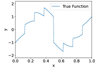
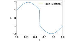
In this section, we perform numerical experiments on 1D piecewise smooth functions, which fit in Example 2a. The following functions are included in our experiments:

  • Function with 1 discontinuity point,

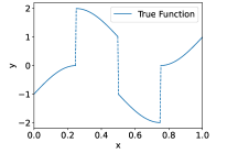
    f(x)={sin(2πx)+1 when 0x<12,sin(2πx)1 when 12x<1.f(x)=\begin{cases}\sin\left(2\pi x\right)+1&\text{ when }0\leq x<\frac{1}{2},\\ \sin\left(2\pi x\right)-1&\text{ when }\frac{1}{2}\leq x<1.\end{cases}
  • Function with 3 discontinuity points,

    f(x)={sin(2πx)1 when 0x<14,sin(2πx)+1 when 14x<12,sin(2πx)1 when 12x<34,sin(2πx)+1 when 34x<1.f(x)=\begin{cases}\sin\left(2\pi x\right)-1&\text{ when }0\leq x<\frac{1}{4},\\ \sin\left(2\pi x\right)+1&\text{ when }\frac{1}{4}\leq x<\frac{1}{2},\\ \sin\left(2\pi x\right)-1&\text{ when }\frac{1}{2}\leq x<\frac{3}{4},\\ \sin\left(2\pi x\right)+1&\text{ when }\frac{3}{4}\leq x<1.\end{cases}
  • Function with 5 discontinuity points,

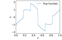
    f(x)={sin(2πx)1 when 0x<16,sin(2πx) when 16x<13,sin(2πx)+1 when 13x<12,sin(2πx)1 when 12x<1,sin(2πx) when 23x<23,sin(2πx)+1 when 56x<1.f(x)=\begin{cases}\sin\left(2\pi x\right)-1&\text{ when }0\leq x<\frac{1}{6},\\ \sin\left(2\pi x\right)&\text{ when }\frac{1}{6}\leq x<\frac{1}{3},\\ \sin\left(2\pi x\right)+1&\text{ when }\frac{1}{3}\leq x<\frac{1}{2},\\ \sin\left(2\pi x\right)-1&\text{ when }\frac{1}{2}\leq x<1,\\ \sin\left(2\pi x\right)&\text{ when }\frac{2}{3}\leq x<\frac{2}{3},\\ \sin\left(2\pi x\right)+1&\text{ when }\frac{5}{6}\leq x<1.\end{cases}
  • Function with 7 discontinuity points,
    f(x)={sin(2πx)1 when 0x<18,sin(2πx)13 when 18x<14,sin(2πx)+13 when 14x<38,sin(2πx)+1 when 38x<12,sin(2πx)1 when 12x<58,sin(2πx)13 when 58x<34,sin(2πx)+13 when 34x<78,sin(2πx)+1 when 78x<1.f(x)=\begin{cases}\sin\left(2\pi x\right)-1&\text{ when }0\leq x<\frac{1}{8},\\ \sin\left(2\pi x\right)-\frac{1}{3}&\text{ when }\frac{1}{8}\leq x<\frac{1}{4},\\ \sin\left(2\pi x\right)+\frac{1}{3}&\text{ when }\frac{1}{4}\leq x<\frac{3}{8},\\ \sin\left(2\pi x\right)+1&\text{ when }\frac{3}{8}\leq x<\frac{1}{2},\\ \sin\left(2\pi x\right)-1&\text{ when }\frac{1}{2}\leq x<\frac{5}{8},\\ \sin\left(2\pi x\right)-\frac{1}{3}&\text{ when }\frac{5}{8}\leq x<\frac{3}{4},\\ \sin\left(2\pi x\right)+\frac{1}{3}&\text{ when }\frac{3}{4}\leq x<\frac{7}{8},\\ \sin\left(2\pi x\right)+1&\text{ when }\frac{7}{8}\leq x<1.\end{cases}
Refer to caption
Refer to caption
Refer to caption
Refer to caption
Figure 4: Functions with different numbers of discontinuity points.
Refer to caption
(a) σ=0,n=16\sigma=0,n=16
Refer to caption
(b) σ=0,n=64\sigma=0,n=64
Refer to caption
(c) σ=0,n=256\sigma=0,n=256
Refer to caption
(d) σ=0.1,n=16\sigma=0.1,n=16
Refer to caption
(e) σ=0.1,n=64\sigma=0.1,n=64
Refer to caption
(f) σ=0.1,n=256\sigma=0.1,n=256
Refer to caption
(g) σ=0.3,n=16\sigma=0.3,n=16
Refer to caption
(h) σ=0.3,n=64\sigma=0.3,n=64
Refer to caption
(i) σ=0.3,n=256\sigma=0.3,n=256
Refer to caption
(j) σ=0.5,n=16\sigma=0.5,n=16
Refer to caption
(k) σ=0.5,n=64\sigma=0.5,n=64
Refer to caption
(l) σ=0.5,n=256\sigma=0.5,n=256
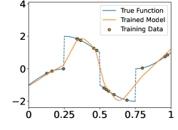
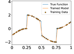
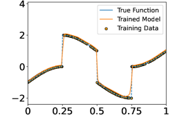
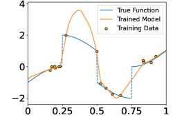
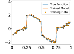
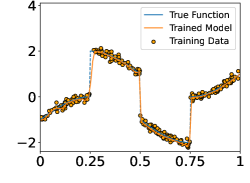
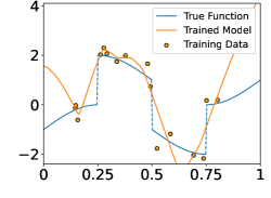
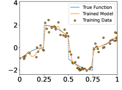
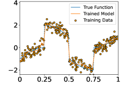
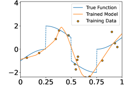
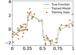
Figure 5: Trained model with ntrain=16n_{\rm train}=16 (1st column), 6464 (2nd column), 256256 (3rd column) when σ=0\sigma=0 (1st row), 0.10.1 (2nd row), 0.30.3 (3rd row), and 0.50.5 (4th row).
Refer to caption
(a) σ=0\sigma=0
Refer to caption
(b) σ=0.1\sigma=0.1
Refer to caption
(c) σ=0.3\sigma=0.3
Refer to caption
(d) σ=0.5\sigma=0.5
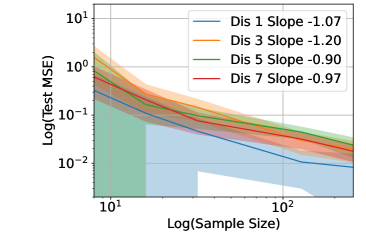
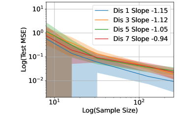
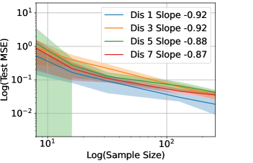
Figure 6: Test MSE versus ntrainn_{\rm train} in log\log-log\log scale for the regression of functions with different number of discontinuity points (Dis) shown in Figure 4, when σ=0\sigma=0(a), σ=0.1\sigma=0.1(b), σ=0.3\sigma=0.3(c) and σ=0.5\sigma=0.5(d). We repeat 20 experiments for each setting. The curve represents the average test MSE in 20 experiments and the shade represents the standard deviation. A least-square fit of the curve gives rise to the slope in the legend.

These functions are shown in the Figure 4. In each experiment, we sample ntrainn_{\rm train} i.i.d. training samples {xi,yi}i=1ntrain\{x_{i},y_{i}\}_{i=1}^{n_{\rm train}} according to the model in (19). Specifically, the xix_{i}’s are independently and uniformly sampled in [0,1][0,1], and yi=f(xi)+ξiy_{i}=f(x_{i})+\xi_{i} with ξi𝒩(0,σ2)\xi_{i}\sim\mathcal{N}(0,\sigma^{2}) being a normal random variable with zero mean and standard deviation σ\sigma. Given the training data, we train a neural network through

f^=argminfNN1ntraini=1ntrain|fNN(xi)yi|2,\displaystyle\widehat{f}=\mathop{\mathrm{argmin}}_{f_{\rm NN}\in\mathcal{F}}\frac{1}{n_{\rm train}}\sum_{i=1}^{n_{\rm train}}|f_{\rm NN}(x_{i})-y_{i}|^{2}, (25)

where the ReLU neural network class \mathcal{F} comprises four fully connected layer (64, 128, 64 neurons in each hidden layer). All weight and bias parameters are initialized with a uniform distribution, and we use Adam optimizer with learning rate 0.0010.001 for training.

Figure 5 shows the ground-truth, training data, and the trained model with different number of training data and noise levels. When σ\sigma is fixed, the trained model approaches the ground-truth function when ntrainn_{\rm train} increases, which is consistent with Theorem 2.

The test mean squared error (MSE) is evaluated on the test samples {xj,f(xj)}ntest\{x_{j},f(x_{j})\}_{n_{\rm test}}

Test MSE=1ntestj=1ntest|f^(xj)f(xj)|2\displaystyle\text{Test MSE}=\frac{1}{n_{\rm test}}\sum_{j=1}^{n_{\rm test}}|\widehat{f}(x_{j})-f(x_{j})|^{2}

with ntest=10,000n_{\rm test}=10,000. We use a large ntestn_{\rm test} in order to reduced the variance in the evaluation of the test MSE.

Figure 6 shows the Test MSE versus ntrainn_{\rm train} in log\log-log\log scale for the regression of functions with different number of discontinuity points shown in Figure 4, when σ=0\sigma=0 in (a), σ=0.1\sigma=0.1 in (b), σ=0.3\sigma=0.3 in (c) and σ=0.5\sigma=0.5 in (d), respectively. We repeat 20 experiments for each setting. The curve represents the average test MSE in 20 experiments and the shade represents the standard deviation. A least-square fit of the curve gives rise to the slope in the legend. These functions fit in Example 2c, which follows Test MSEntrain2r2r+1log3n\text{Test MSE}\lesssim{n_{\rm train}}^{-\frac{2r}{2r+1}}\log^{3}n for a large rr since the functions are smooth except at the discontinuity points. Our Example 2c predicts the slope about 1-1 in the log\log-log\log plot of test MSE versus ntrainn_{\rm train}, and the slope is not sensitive to the number of (finite) discontinuity points. The numerical slopes in Figure 6 are consistent with our theory.

6 Proof of main results

In this section, we present the proof of our main results. Some preliminaries for the proof are introduced in Subsection 6.1. Theorem 1 is proved in Subsection 6.2 and Theorem 2 is proved in Subsection 6.3.

6.1 Proof preliminaries

We first introduce some preliminaries to be used in the proof.

6.1.1 Trapezoidal function and its neural network representation

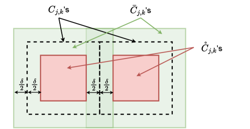
Given an interval [a,b][0,1][a,b]\subset[0,1] and 0<δ<ba0<\delta<b-a, the function defined as

ψ[a,b](x)={0 if x<aδ/2,x(aδ/2)δ if aδ/2xa+δ/2,1 if a+δ/2<x<bδ/2,1x(bδ/2)δ if bδ/2xb+δ/2,0 if x>b+δ/2,\displaystyle\psi_{[a,b]}(x)=\begin{cases}0&\mbox{ if }x<a-\delta/2,\\ \frac{x-(a-\delta/2)}{\delta}&\mbox{ if }a-\delta/2\leq x\leq a+\delta/2,\\ 1&\mbox{ if }a+\delta/2<x<b-\delta/2,\\ 1-\frac{x-(b-\delta/2)}{\delta}&\mbox{ if }b-\delta/2\leq x\leq b+\delta/2,\\ 0&\mbox{ if }x>b+\delta/2,\end{cases} for a0,b1,\displaystyle\mbox{ for }\quad a\neq 0,\ b\neq 1,
ψ[a,b](x)={1 if ax<bδ/2,1x(bδ/2)δ if bδ/2xb+δ/2,0 if x>b+δ/2,\displaystyle\psi_{[a,b]}(x)=\begin{cases}1&\mbox{ if }a\leq x<b-\delta/2,\\ 1-\frac{x-(b-\delta/2)}{\delta}&\mbox{ if }b-\delta/2\leq x\leq b+\delta/2,\\ 0&\mbox{ if }x>b+\delta/2,\end{cases} for a=0,\displaystyle\mbox{ for }a=0,
ψ[a,b](x)={0 if x<aδ/2,x(aδ/2)δ if aδ/2xa+δ/2,1 if a+δ/2<xb\displaystyle\psi_{[a,b]}(x)=\begin{cases}0&\mbox{ if }x<a-\delta/2,\\ \frac{x-(a-\delta/2)}{\delta}&\mbox{ if }a-\delta/2\leq x\leq a+\delta/2,\\ 1&\mbox{ if }a+\delta/2<x\leq b\end{cases} for b=1\displaystyle\mbox{ for }b=1 (26)

is piecewise linear and supported on [aδ/2,b+δ/2][a-\delta/2,b+\delta/2] (or [a,b+δ/2][a,b+\delta/2] or [aδ/2,b][a-\delta/2,b]). In the rest of the proof, for simplicity, we only discuss the case for 0<a<b<10<a<b<1. The case for a=0a=0 or b=1b=1 can be derived similarly. Function ψ[a,b]\psi_{[a,b]} can be realized by the following ReLU network with 1 layer and width 4:

ψ~[a,b](x)=1δ(\displaystyle\widetilde{\psi}_{[a,b]}(x)=\frac{1}{\delta}\Big{(} ReLU(x(aδ/2))ReLU(x(a+δ/2))\displaystyle\mathrm{ReLU}(x-(a-\delta/2))-\mathrm{ReLU}(x-(a+\delta/2))
ReLU(x(bδ/2)+ReLU(x(b+δ/2))).\displaystyle-\mathrm{ReLU}(x-(b-\delta/2)+\mathrm{ReLU}(x-(b+\delta/2))\Big{)}.

6.1.2 Multiplication operation and neural network approximation

The following lemma from Yarotsky (2017) shows that the product operation can be well approximated by a ReLU network.

Lemma 2 (Proposition 3 in Yarotsky (2017)).

For any C>0C>0 and 0<ε<10<\varepsilon<1. If |x|C,|y|C|x|\leq C,|y|\leq C, there is a ReLU network, denoted by ×~(,)\widetilde{\times}(\cdot,\cdot), such that

|×~(x,y)xy|<ε,\displaystyle|\widetilde{\times}(x,y)-xy|<\varepsilon,
×~(x,0)=\displaystyle\widetilde{\times}(x,0)= ×~(y,0)=0,|×~(x,y)|C2.\displaystyle\widetilde{\times}(y,0)=0,\ |\widetilde{\times}(x,y)|\leq C^{2}.

Such a network has O(log1ε)O\left(\log\frac{1}{\varepsilon}\right) layers and parameters, where the constants hidden in OO depends on CC. The width of each layer is bounded by 6 and all parameters are bounded by O(C2)O(C^{2}), where the constant hidden in OO is an absolute constant.

Furthermore, the following lemma shows that composition of products can be well approximated by a ReLU network (see a proof in Appendix C)

Lemma 3.

Let {ai}i=1N\{a_{i}\}_{i=1}^{N} be a set of real numbers satisfying |ai|C|a_{i}|\leq C for any ii. For any 0<ε<10<\varepsilon<1, there exists a neural network Π~NN(L,w,K,κ,M)\widetilde{\Pi}\in\mathcal{F}_{\rm NN}(L,w,K,\kappa,M) such that

|Π~(a1,,aN)i=1Nai|Nε.\displaystyle|\widetilde{\Pi}(a_{1},...,a_{N})-\prod_{i=1}^{N}a_{i}|\leq N\varepsilon.

The network NN(L,w,K,κ,M)\mathcal{F}_{\rm NN}(L,w,K,\kappa,M) has

L=O(Nlog1ε),w=N+6,K=O(Nlog1ε),κ=O(CN),M=CN,\displaystyle L=O\left(N\log\frac{1}{\varepsilon}\right),w=N+6,K=O\left(N\log\frac{1}{\varepsilon}\right),\kappa=O(C^{N}),M=C^{N}, (27)

where the constant hidden in OO of LL and KK depends on CC, and κ\kappa is some absolute constant.

6.2 Proof of Theorem 1

Proof of Theorem 1.

To prove Theorem 1, we first decompose the approximation error into two parts by applying the triangle inequality with the piecewise polynomial on the adaptive partition pΛ(f,η)p_{\Lambda(f,\eta)} defined in (7). The first part is the approximation error of ff by pΛ(f,η)p_{\Lambda(f,\eta)}, which can be bounded by (10). The second part is the network approximation error of pΛ(f,η)p_{\Lambda(f,\eta)}. Then we show that pΛ(f,η)p_{\Lambda(f,\eta)} can be approximated by the given neural network with an arbitrary accuracy. Lastly, we estimate the total approximation error and quantify the network size. In the following we present the details of each step.

\bullet Decomposition of the approximation error. For any f~\widetilde{f} given by the network in (17), we decompose the error as

f~fL2(ρ)22fpΛ(f,η)L2(ρ)2+2f~pΛ(f,η)L2(ρ)2,\displaystyle\|\widetilde{f}-f\|_{L^{2}(\rho)}^{2}\leq 2\|f-p_{\Lambda(f,\eta)}\|_{L^{2}(\rho)}^{2}+2\|\widetilde{f}-p_{\Lambda(f,\eta)}\|_{L^{2}(\rho)}^{2}, (28)

where η>0\eta>0 is to be determined later. The first term in (28) can be bounded by (10) such that

2fpΛ(f,η)L2(ρ)22CsR𝒜2(#𝒯(f,η))2s.\displaystyle 2\|f-p_{\Lambda(f,\eta)}\|_{L^{2}(\rho)}^{2}\leq 2C_{s}R_{\mathcal{A}}^{2}(\#\mathcal{T}(f,\eta))^{-{2s}}. (29)

\bullet Bounding the second term in (28). We next derive an upper bound for the second term in (28) by showing that pΛ(f,η)p_{\Lambda(f,\eta)} can be well approximated by a network f~\widetilde{f}. This part contains four steps:

Step 1

Estimate the finest scale of the truncated tree.

Step 2

Construct a partition of unity of XX with respect to the truncated tree. Each element of the partition of unity is a network.

Step 3

Based on the partition of unity, construct a network to approximate pj,kp_{j,k} on each cube.

Step 4

Estimate the approximation error.

In the following we disucss details of each step.

— Step 1: Estimate the finest scale. Denote the truncated tree and its outer leaves of pΛ(f,η)p_{\Lambda(f,\eta)} by 𝒯{\mathcal{T}} and Λ\Lambda respectively for simplicity. Each Cj,kΛC_{j,k}\in\Lambda is a hypercube in the form of =1d[r,j,k,r,j,k+2j]\otimes_{\ell=1}^{d}[r_{\ell,j,k},r_{\ell,j,k}+2^{-j}], where r,j,k[0,1]r_{\ell,j,k}\in[0,1] are scalars and

=1d[r,j,k,r,j,k+2j]=[r1,j,k,r1,j,k+2j]××[rd,j,k,rd,j,k+2j]\displaystyle\otimes_{\ell=1}^{d}[r_{\ell,j,k},r_{\ell,j,k}+2^{-j}]=[r_{1,j,k},r_{1,j,k}+2^{-j}]\times\cdots\times[r_{d,j,k},r_{d,j,k}+2^{-j}]

is a hypercube with edge length 2j2^{-j} in d\mathbb{R}^{d}.

We estimate the finest scale in Λ\Lambda. Let J>0J>0 be the largest integer such that CJ,kΛC_{J,k}\in\Lambda for some kk. In other words, 2J2^{-J} is the finest scale of the cubes in Λ(f,η)\Lambda(f,\eta). Let C1=R𝒜mC_{1}=R_{\mathcal{A}}^{m} so that

supη>0ηm#𝒯(f,η)R𝒜m=C1,\displaystyle\sup_{\eta>0}\eta^{m}\#{\mathcal{T}}(f,\eta)\leq R_{\mathcal{A}}^{m}=C_{1},

with the mm given in (8), which implies

η(C1#𝒯(f,η))1m.\displaystyle\eta\leq\left(\frac{C_{1}}{\#{\mathcal{T}}(f,\eta)}\right)^{\frac{1}{m}}. (30)

For any Cj,kΛ(f,η)C_{j,k}\in\Lambda(f,\eta) and its parent Cj1,kC_{j-1,k^{\prime}}, we have δj1,k>η\delta_{j-1,k^{\prime}}>\eta. Meanwhile, we have

δj1,k2Cρ12fL(X)|Cj1,k|2Cρ12R2(j1)d/2.\delta_{j-1,k^{\prime}}\leq 2C^{\frac{1}{2}}_{\rho}\|f\|_{L^{\infty}(X)}|C_{j-1,k^{\prime}}|\leq 2C_{\rho}^{\frac{1}{2}}R2^{-(j-1)d/2}.

This implies

j<2dlog2η2Cρ12R+1.\displaystyle j<-\frac{2}{d}\log_{2}\frac{\eta}{2C_{\rho}^{\frac{1}{2}}R}+1. (31)

Substituting (30) into (31) gives rise to

j2mdlog#𝒯(f,η)2mdlogC1+1+2dlog2(2Cρ12R)C2log#𝒯(f,η),\displaystyle j\leq\frac{2}{md}\log\#{\mathcal{T}}(f,\eta)-\frac{2}{md}\log C_{1}+1+\frac{2}{d}\log_{2}(2C_{\rho}^{\frac{1}{2}}R)\leq C_{2}\log\#{\mathcal{T}}(f,\eta), (32)

where C2C_{2} is a constant depending on d,m,Cρd,m,C_{\rho} and RR. Since (32) holds for any Cj,kΛ(f,η)C_{j,k}\in\Lambda(f,\eta), we have

JC2log#𝒯(f,η).\displaystyle J\leq C_{2}\log\#{\mathcal{T}}(f,\eta). (33)

— Step 2: Construct a partition of unity. Let 0<δ2(J+2)0<\delta\leq 2^{-(J+2)}. For each Cj,kΛ(f,η)C_{j,k}\in\Lambda(f,\eta), we define two sets:

C̊j,k==1d[r,j,k+δ/2,r,j,k+2jδ/2]X,\displaystyle\mathring{C}_{j,k}=\otimes_{\ell=1}^{d}[r_{\ell,j,k}+\delta/2,r_{\ell,j,k}+2^{-j}-\delta/2]\cap X,
C¯j,k=(=1d[r,j,kδ/2,r,j,k+2j+δ/2]X)\C̊j,k.\displaystyle\bar{C}_{j,k}=\left(\otimes_{\ell=1}^{d}[r_{\ell,j,k}-\delta/2,r_{\ell,j,k}+2^{-j}+\delta/2]\cap X\right)\backslash\mathring{C}_{j,k}. (34)

The C̊j,k\mathring{C}_{j,k} set is in the interior of Cj,kC_{j,k}, with δ/2\delta/2 distance to the boundary of Cj,kC_{j,k}. The C¯j,k\bar{C}_{j,k} set contains the boundary of Cj,kC_{j,k}. The relations of C¯j,k,C̊j,k\bar{C}_{j,k},\mathring{C}_{j,k} and Cj,kC_{j,k} are illustrated in Figure 7.

Refer to caption
Figure 7: An illustration of the relation among Cj,k,C̊j,kC_{j,k},\mathring{C}_{j,k} and C¯j,k\bar{C}_{j,k}.

For each Cj,kC_{j,k}, we define the function

ϕj,k(𝐱)==1dψ[r,j,k,r,j,k+2j](x),\displaystyle\phi_{j,k}(\mathbf{x})=\prod_{\ell=1}^{d}\psi_{[r_{\ell,j,k},r_{\ell,j,k}+2^{-j}]}(x_{\ell}),

where 𝐱=[x1,,xd]\mathbf{x}=[x_{1},...,x_{d}]^{\top}, and the ψ\psi function is defined in (26). The function ϕj,k\phi_{j,k} has the following properties:

  1. 1.

    ϕj,k\phi_{j,k} is piecewise linear.

  2. 2.

    ϕj,k\phi_{j,k} is supported on C̊j,kC¯j,k\mathring{C}_{j,k}\cup\bar{C}_{j,k}, and ϕj,k(𝐱)=1\phi_{j,k}(\mathbf{x})=1 when 𝐱C̊j,k\mathbf{x}\in\mathring{C}_{j,k}.

  3. 3.

    The ϕj,k\phi_{j,k}’s form a partition of unity of XX: Cj,kΛϕj,k(𝐱)=1\sum_{C_{j,k}\in\Lambda}\phi_{j,k}(\mathbf{x})=1 when 𝐱X=[0,1]d\mathbf{x}\in X=[0,1]^{d}.

In this paper, we approximate ϕj,k(𝐱)\phi_{j,k}(\mathbf{x}) by

ϕ~j,k(𝐱)=\displaystyle\widetilde{\phi}_{j,k}(\mathbf{x})= Π~(ψ[r1,j,k,r1,j,k+2j](x1),ψ[r2,j,k,r2,j,k+2j](x2),,ψ[rd,j,k,rd,j,k+2j](xd)),\displaystyle\widetilde{\Pi}\bigg{(}\psi_{[r_{1,j,k},r_{1,j,k}+2^{-j}]}(x_{1}),\psi_{[r_{2,j,k},r_{2,j,k}+2^{-j}]}(x_{2}),\cdots,\psi_{[r_{d,j,k},r_{d,j,k}+2^{-j}]}(x_{d})\bigg{)},

where the network Π~\widetilde{\Pi} with dd inputs is defined in Lemma 3 with accuracy dε1d\varepsilon_{1}. We have ϕ~j,k1=(L1,w1,K1,κ1,M1)\widetilde{\phi}_{j,k}\in\mathcal{F}_{1}=\mathcal{F}(L_{1},w_{1},K_{1},\kappa_{1},M_{1}) with

L1=O(dlog1ε1),w1=d+6,K1=O(dlog1ε1),κ1=O(1δ),M1=1.\displaystyle L_{1}=O\left(d\log\frac{1}{\varepsilon_{1}}\right),w_{1}=d+6,K_{1}=O\left(d\log\frac{1}{\varepsilon_{1}}\right),\kappa_{1}=O\left(\frac{1}{\delta}\right),M_{1}=1.

By Lemma 3, we have

sup𝐱[0,1]d|ϕ~j,k(𝐱)ϕj,k(𝐱)|dε1.\displaystyle\sup_{\mathbf{x}\in[0,1]^{d}}|\widetilde{\phi}_{j,k}(\mathbf{x})-\phi_{j,k}(\mathbf{x})|\leq d\varepsilon_{1}. (35)

— Step 3: Approximate pj,kp_{j,k} on each cube. According to (15), for each Cj,kΛ(f,η)C_{j,k}\in\Lambda(f,\eta), pj,k(f)p_{j,k}(f) is a polynomial of degree θ\theta and is in the form of

pj,k=|𝜶|θa𝜶(2j(𝐱𝐫j,k))𝜶,\displaystyle p_{j,k}=\sum_{|\bm{\alpha}|\leq\theta}a_{\bm{\alpha}}(2^{j}(\mathbf{x}-\mathbf{r}_{j,k}))^{\bm{\alpha}}, (36)

where 𝐫j,k=[r1,j,k,,rd,j,k]\mathbf{r}_{j,k}=[r_{1,j,k},...,r_{d,j,k}]^{\top}.

We approximate pj,kp_{j,k} by

p~j,k(𝐱)=|𝜶|θa𝜶Π~(2j(x1r1,j,k),,2j(x1r1,j,k)α1 times ,,2j(xdrd,j,k),,2j(xdrd,j,k)αd times ),\displaystyle\widetilde{p}_{j,k}(\mathbf{x})=\sum_{|\bm{\alpha}|\leq\theta}a_{\bm{\alpha}}\widetilde{\Pi}(\underbrace{2^{j}(x_{1}-r_{1,j,k}),...,2^{j}(x_{1}-r_{1,j,k})}_{\alpha_{1}\mbox{ times }},...,\underbrace{2^{j}(x_{d}-r_{d,j,k}),...,2^{j}(x_{d}-r_{d,j,k})}_{\alpha_{d}\mbox{ times }}),

where Π~(2j(x1r1,j,k),,2j(x1r1,j,k)α1 times ,,2j(xdrd,j,k),,2j(xdrd,j,k)αd times )\widetilde{\Pi}(\underbrace{2^{j}(x_{1}-r_{1,j,k}),...,2^{j}(x_{1}-r_{1,j,k})}_{\alpha_{1}\mbox{ times }},...,\underbrace{2^{j}(x_{d}-r_{d,j,k}),...,2^{j}(x_{d}-r_{d,j,k})}_{\alpha_{d}\mbox{ times }}) is the network approximation of (2j(𝐱𝐫j,k))𝜶(2^{j}(\mathbf{x}-\mathbf{r}_{j,k}))^{\bm{\alpha}} with accuracy θε1\theta\varepsilon_{1}, according to Lemma 3.

By Assumption 2(ii), there exists Rp>0R_{p}>0 so that |a𝜶||a_{\bm{\alpha}}| is uniformly bounded by RpR_{p} for any |𝜶|θ|\bm{\alpha}|\leq\theta for any pj,kp_{j,k}. By Lemma 3, we have

|p~j,k(𝐱)pj,k(𝐱)|\displaystyle|\widetilde{p}_{j,k}(\mathbf{x})-p_{j,k}(\mathbf{x})|
\displaystyle\leq |𝜶|θa𝜶|Π~(2j(x1r1,j,k),,2j(x1r1,j,k)α1 times ,,2j(xdrd,j,k),,2j(xdrd,j,k)αd times )(2j(𝐱𝐫j,k))𝜶|\displaystyle\sum_{|\bm{\alpha}|\leq\theta}a_{\bm{\alpha}}\left|\widetilde{\Pi}(\underbrace{2^{j}(x_{1}-r_{1,j,k}),...,2^{j}(x_{1}-r_{1,j,k})}_{\alpha_{1}\mbox{ times }},...,\underbrace{2^{j}(x_{d}-r_{d,j,k}),...,2^{j}(x_{d}-r_{d,j,k})}_{\alpha_{d}\mbox{ times }})-(2^{j}(\mathbf{x}-\mathbf{r}_{j,k}))^{\bm{\alpha}}\right|
\displaystyle\leq C3Rpθε1\displaystyle C_{3}R_{p}\theta\varepsilon_{1} (37)

for some C3C_{3} dpending on d,θd,\theta, and p~j,k2=(L2,w2,K2,κ2,M2)\widetilde{p}_{j,k}\in\mathcal{F}_{2}=\mathcal{F}(L_{2},w_{2},K_{2},\kappa_{2},M_{2}) with

L2=O(θlog1ε1),w2=O(θdθ),K2=O(θdθlog1ε1),κ2=O(2J),M2=R.\displaystyle L_{2}=O(\theta\log\frac{1}{\varepsilon_{1}}),\ w_{2}=O(\theta d^{\theta}),\ K_{2}=O(\theta d^{\theta}\log\frac{1}{\varepsilon_{1}}),\ \kappa_{2}=O(2^{J}),\ M_{2}=R.

— Step 4: Estimate the network approximation error for pΛ(f,η)p_{\Lambda(f,\eta)}. We approximate

pΛ(f,η)(𝐱)=Cj,kΛ(f,η)pj,k(𝐱)p_{\Lambda(f,\eta)}(\mathbf{x})=\sum_{C_{j,k}\in\Lambda(f,\eta)}p_{j,k}(\mathbf{x})

by

f~(𝐱)=Cj,kΛ(f,η)×~(ϕ~j,k(𝐱),p~j,k(𝐱)),\displaystyle\widetilde{f}(\mathbf{x})=\sum_{C_{j,k}\in\Lambda(f,\eta)}\widetilde{\times}(\widetilde{\phi}_{j,k}(\mathbf{x}),\widetilde{p}_{j,k}(\mathbf{x})), (38)

where ×~\widetilde{\times} is the product network with accuracy ε1\varepsilon_{1}, according to Lemma 2.

Denote X1=Cj,kΛ(f,η)C̊j,k,X2=Cj,kΛ(f,η)C¯j,kX_{1}=\cup_{C_{j,k}\in\Lambda(f,\eta)}\mathring{C}_{j,k},\ X_{2}=\cup_{C_{j,k}\in\Lambda(f,\eta)}\bar{C}_{j,k}. The error is estimated as

f~pΛ(f,η)L2(X)2=f~pΛ(f,η)L2(X1)2+f~pΛ(f,η)L2(X2)2.\displaystyle\|\widetilde{f}-p_{\Lambda(f,\eta)}\|_{L^{2}(X)}^{2}=\|\widetilde{f}-p_{\Lambda(f,\eta)}\|_{L^{2}(X_{1})}^{2}+\|\widetilde{f}-p_{\Lambda(f,\eta)}\|_{L^{2}(X_{2})}^{2}. (39)

For the first term in (39), we have

f~pΛ(f,η)L2(X1)2\displaystyle\|\widetilde{f}-p_{\Lambda(f,\eta)}\|_{L^{2}(X_{1})}^{2} (40)
=\displaystyle= Cj,kΛ(f,η)C̊j,k|×~(ϕ~j,k(𝐱),p~j,k(𝐱))pj,k(𝐱)|2𝑑𝐱\displaystyle\sum_{C_{j,k}\in\Lambda(f,\eta)}\int_{\mathring{C}_{j,k}}|\widetilde{\times}(\widetilde{\phi}_{j,k}(\mathbf{x}),\widetilde{p}_{j,k}(\mathbf{x}))-p_{j,k}(\mathbf{x})|^{2}d\mathbf{x}
\displaystyle\leq Cj,kΛ(f,η)C̊j,k3[|×~(ϕ~j,k(𝐱),p~j,k(𝐱))ϕ~j,k(𝐱)p~j,k(𝐱)|2\displaystyle\sum_{C_{j,k}\in\Lambda(f,\eta)}\int_{\mathring{C}_{j,k}}3\Big{[}|\widetilde{\times}(\widetilde{\phi}_{j,k}(\mathbf{x}),\widetilde{p}_{j,k}(\mathbf{x}))-\widetilde{\phi}_{j,k}(\mathbf{x})\widetilde{p}_{j,k}(\mathbf{x})|^{2}
+|ϕ~j,k(𝐱)p~j,k(𝐱)ϕj,k(𝐱)p~j,k(𝐱)|2+|ϕj,k(𝐱)p~j,k(𝐱)pj,k(𝐱)|2]d𝐱\displaystyle+|\widetilde{\phi}_{j,k}(\mathbf{x})\widetilde{p}_{j,k}(\mathbf{x})-\phi_{j,k}(\mathbf{x})\widetilde{p}_{j,k}(\mathbf{x})|^{2}+|\phi_{j,k}(\mathbf{x})\widetilde{p}_{j,k}(\mathbf{x})-p_{j,k}(\mathbf{x})|^{2}\Big{]}d\mathbf{x}
\displaystyle\leq Cj,kΛ(f,η)C̊j,k3[ε12+R2d2ε12+|p~j,k(𝐱)pj,k(𝐱)|2]𝑑𝐱\displaystyle\sum_{C_{j,k}\in\Lambda(f,\eta)}\int_{\mathring{C}_{j,k}}3\Big{[}\varepsilon_{1}^{2}+R^{2}d^{2}\varepsilon_{1}^{2}+|\widetilde{p}_{j,k}(\mathbf{x})-p_{j,k}(\mathbf{x})|^{2}\Big{]}d\mathbf{x}
\displaystyle\leq 3(R2d2+1+C32Rp2θ2)ε12Cj,kΛ(f,η)|C̊j,k|\displaystyle 3(R^{2}d^{2}+1+C_{3}^{2}R_{p}^{2}\theta^{2})\varepsilon_{1}^{2}\sum_{C_{j,k}\in\Lambda(f,\eta)}|\mathring{C}_{j,k}|
\displaystyle\leq 3(R2d2+1+C32Rp2θ2)ε12.\displaystyle 3(R^{2}d^{2}+1+C_{3}^{2}R_{p}^{2}\theta^{2})\varepsilon_{1}^{2}. (41)

In the derivation above, we used ϕj,k(𝒙)=1\phi_{j,k}(\bm{x})=1 when 𝐱C̊j,k\mathbf{x}\in\mathring{C}_{j,k}. Additionally, (35) is used in the second inequality, (37) is used in the third inequality.

We next derive an upper bound for the second term in (39) by bounding the volume of X2X_{2}. We define the common boundaries of a set of cubes being the outer leaves of a truncated tree as the set of points that belong to at least two cubes. We will use the following lemma to estimate the surface area for the common boundaries of Λ(f,η)\Lambda(f,\eta) (see a proof in Appendix D).

Lemma 4.

Given a truncated tree 𝒯{\mathcal{T}} and its outer leaves Λ𝒯\Lambda_{{\mathcal{T}}}, we denote the set of common boundaries of the subcubes in Λ𝒯\Lambda_{{\mathcal{T}}} by (Λ𝒯)\mathcal{B}(\Lambda_{{\mathcal{T}}}). The surface area of (Λ𝒯)\mathcal{B}(\Lambda_{{\mathcal{T}}}) in d1\mathbb{R}^{d-1}, denoted by |(Λ𝒯)||\mathcal{B}(\Lambda_{{\mathcal{T}}})|, satisfies

|(Λ𝒯)|2d+1d(#𝒯)1/d.\displaystyle|\mathcal{B}(\Lambda_{{\mathcal{T}}})|\leq 2^{d+1}d(\#{\mathcal{T}})^{1/d}. (42)

By Lemma 4 and Assumption 1, we have

f~pΛ(f,η)L2(X2)24R2|X2|4R2δ|(Λ𝒯)|2d+3dR2δ(#𝒯)1/d.\displaystyle\|\widetilde{f}-p_{\Lambda(f,\eta)}\|_{L^{2}(X_{2})}^{2}\leq 4R^{2}|X_{2}|\leq 4R^{2}\delta|\mathcal{B}(\Lambda_{{\mathcal{T}}})|\leq 2^{d+3}dR^{2}\delta(\#{\mathcal{T}})^{1/d}. (43)

Putting (41) and (43) together, we have

f~pΛ(f,η)L2(X)23(R2d2+1+C32Rp2θ2)ε12+2d+3dR2δ(#𝒯)1/d.\displaystyle\|\widetilde{f}-p_{\Lambda(f,\eta)}\|_{L^{2}(X)}^{2}\leq 3(R^{2}d^{2}+1+C_{3}^{2}R_{p}^{2}\theta^{2})\varepsilon_{1}^{2}+2^{d+3}dR^{2}\delta(\#{\mathcal{T}})^{1/d}. (44)

\bullet Putting all terms together. Set ε1=(#𝒯)s,δ=min{(#𝒯)2s1/d,2ζ2}\varepsilon_{1}=(\#{\mathcal{T}})^{-s},\delta=\min\{(\#{\mathcal{T}})^{-2s-1/d},2^{-\zeta-2}\}, and substitute (44) and (29) into (28) gives rise to

f~fL2(X)2\displaystyle\|\widetilde{f}-f\|_{L^{2}(X)}^{2}\leq 2CsR𝒜2(#𝒯(f,η))2s+6(R2d2+1+C32Rp2θ2)ε12+2d+3dR2δ#𝒯1/d\displaystyle 2C_{s}R_{\mathcal{A}}^{2}(\#\mathcal{T}(f,\eta))^{-{2s}}+6(R^{2}d^{2}+1+C_{3}^{2}R_{p}^{2}\theta^{2})\varepsilon_{1}^{2}+2^{d+3}dR^{2}\delta\#{\mathcal{T}}^{1/d}
\displaystyle\leq (2CsR𝒜2+6(R2d2+1+C32Rp2θ2)+2d+3dR2)(#𝒯(f,η))2s.\displaystyle\left(2C_{s}R_{\mathcal{A}}^{2}+6(R^{2}d^{2}+1+C_{3}^{2}R_{p}^{2}\theta^{2})+2^{d+3}dR^{2}\right)(\#\mathcal{T}(f,\eta))^{-{2s}}. (45)

We then quantify the network size of f~\widetilde{f}.

  • \circ

    ×~\widetilde{\times}: The product network has depth O(log1ε1)O(\log\frac{1}{\varepsilon_{1}}), width 66, number of nonzero parameters O(log1ε1)O(\log\frac{1}{\varepsilon_{1}}), and all parameters are bounded by R2R^{2}.

  • \circ

    ϕ~j,k\widetilde{\phi}_{j,k}: Each ϕ~j,k\widetilde{\phi}_{j,k} has depth O(dlog1ε1)O(d\log\frac{1}{\varepsilon_{1}}), width O(1)O(1), number of parameters O(dlog1ε1)O(d\log\frac{1}{\varepsilon_{1}}), and all parameters are bounded by O(1δ)O(\frac{1}{\delta}).

  • \circ

    p~j,k\widetilde{p}_{j,k}: Each p~j,k\widetilde{p}_{j,k} has depth O(θlog1ε1)O(\theta\log\frac{1}{\varepsilon_{1}}), width O(θdθ)O(\theta d^{\theta}), number of parameters O(θdθlog1ε1)O(\theta d^{\theta}\log\frac{1}{\varepsilon_{1}}), and all parameters are bounded by O(2ζ)O(2^{\zeta}).

Substituting the value of ε1\varepsilon_{1} and δ\delta, we get f~(L,w,K,κ,M)\widetilde{f}\in\mathcal{F}(L,w,K,\kappa,M) with

L=O(log#𝒯(f,η)),w=O(#𝒯(f,η)),K=O(#𝒯(f,η)log#𝒯(f,η)),\displaystyle L=O(\log\#{\mathcal{T}}(f,\eta)),\ w=O(\#{\mathcal{T}}(f,\eta)),\ K=O(\#{\mathcal{T}}(f,\eta)\log\#{\mathcal{T}}(f,\eta)),
κ=O((#𝒯(f,η))2s+2ζ),M=R.\displaystyle\kappa=O((\#{\mathcal{T}}(f,\eta))^{2s}+2^{\zeta}),\ M=R. (46)

Note that by (33) we have

2ζ<2C22log#𝒯(f,η)<2C2#𝒯(f,η).\displaystyle 2^{\zeta}<2^{C_{2}}\cdot 2^{\log\#{\mathcal{T}}(f,\eta)}<2^{C_{2}}\#{\mathcal{T}}(f,\eta). (47)

We have κ=O((#𝒯(f,η))max{2s,1})\kappa=O((\#{\mathcal{T}}(f,\eta))^{\max\{2s,1\}}).

Setting

#𝒯(f,η))=(2CsR𝒜2+6(R2d2+1+C32Rp2θ2)+2d+3dR2ε)1s\#\mathcal{T}(f,\eta))=\left(\frac{\sqrt{2C_{s}R_{\mathcal{A}}^{2}+6(R^{2}d^{2}+1+C_{3}^{2}R_{p}^{2}\theta^{2})+2^{d+3}dR^{2}}}{\varepsilon}\right)^{\frac{1}{s}}

finishes the proof. ∎

6.3 Proof of Theorem 2

Proof of Theorem 2.

Let f^\widehat{f} be the minimizer of (20). We decompose the squared generalization error as

𝔼𝒮𝔼𝐱ρ|f^(𝐱)f(𝐱)|2=\displaystyle\mathbb{E}_{{\mathcal{S}}}\mathbb{E}_{\mathbf{x}\sim\rho}|\widehat{f}(\mathbf{x})-f(\mathbf{x})|^{2}= 2𝔼𝒮[1ni=1n(f^(𝐱i)f(𝐱i))2]T1\displaystyle\underbrace{2\mathbb{E}_{{\mathcal{S}}}\left[\frac{1}{n}\sum_{i=1}^{n}(\widehat{f}(\mathbf{x}_{i})-f(\mathbf{x}_{i}))^{2}\right]}_{\rm T_{1}} (48)
+𝔼𝒮[X(f^(𝐱)f(𝐱))2𝑑ρ(𝐱)]2𝔼𝒮[1ni=1n(f^(𝐱i)f(𝐱i))2dρ(𝐱)]T2.\displaystyle+\underbrace{\mathbb{E}_{{\mathcal{S}}}\left[\int_{X}(\widehat{f}(\mathbf{x})-f(\mathbf{x}))^{2}d\rho(\mathbf{x})\right]-2\mathbb{E}_{{\mathcal{S}}}\left[\frac{1}{n}\sum_{i=1}^{n}(\widehat{f}(\mathbf{x}_{i})-f(\mathbf{x}_{i}))^{2}d\rho(\mathbf{x})\right]}_{\rm T_{2}}. (49)

\bullet Bounding T1{\rm T_{1}}. We bound T1{\rm T_{1}} as

T1=\displaystyle{\rm T_{1}}= 2𝔼𝒮[1ni=1n(f^(𝐱i)yi+ξi)2]\displaystyle 2\mathbb{E}_{{\mathcal{S}}}\left[\frac{1}{n}\sum_{i=1}^{n}(\widehat{f}(\mathbf{x}_{i})-y_{i}+\xi_{i})^{2}\right]
=\displaystyle= 2𝔼𝒮[1ni=1n(f^(𝐱i)yi)2]+2𝔼𝒮[1ni=1nξi2]+4𝔼𝒮[1ni=1nξi(f^(𝐱i)yi)]\displaystyle 2\mathbb{E}_{{\mathcal{S}}}\left[\frac{1}{n}\sum_{i=1}^{n}(\widehat{f}(\mathbf{x}_{i})-y_{i})^{2}\right]+2\mathbb{E}_{{\mathcal{S}}}\left[\frac{1}{n}\sum_{i=1}^{n}\xi_{i}^{2}\right]+4\mathbb{E}_{{\mathcal{S}}}\left[\frac{1}{n}\sum_{i=1}^{n}\xi_{i}(\widehat{f}(\mathbf{x}_{i})-y_{i})\right]
=\displaystyle= 2𝔼𝒮[inffNN(1ni=1n(fNN(𝐱i)yi)2)]+2𝔼𝒮[1ni=1nξi2]+4𝔼𝒮[1ni=1nξi(f^(𝐱i)f(𝐱i)ξi)]\displaystyle 2\mathbb{E}_{{\mathcal{S}}}\left[\inf_{f_{\rm NN}\in\mathcal{F}}\left(\frac{1}{n}\sum_{i=1}^{n}(f_{\rm NN}(\mathbf{x}_{i})-y_{i})^{2}\right)\right]+2\mathbb{E}_{{\mathcal{S}}}\left[\frac{1}{n}\sum_{i=1}^{n}\xi_{i}^{2}\right]+4\mathbb{E}_{{\mathcal{S}}}\left[\frac{1}{n}\sum_{i=1}^{n}\xi_{i}(\widehat{f}(\mathbf{x}_{i})-f(\mathbf{x}_{i})-\xi_{i})\right]
=\displaystyle= 2𝔼𝒮[inffNN(1ni=1n(fNN(𝐱i)yi)2)]2𝔼𝒮[1ni=1nξi2]+4𝔼𝒮[1ni=1nξif^(𝐱i))]\displaystyle 2\mathbb{E}_{{\mathcal{S}}}\left[\inf_{f_{\rm NN}\in\mathcal{F}}\left(\frac{1}{n}\sum_{i=1}^{n}(f_{\rm NN}(\mathbf{x}_{i})-y_{i})^{2}\right)\right]-2\mathbb{E}_{{\mathcal{S}}}\left[\frac{1}{n}\sum_{i=1}^{n}\xi_{i}^{2}\right]+4\mathbb{E}_{{\mathcal{S}}}\left[\frac{1}{n}\sum_{i=1}^{n}\xi_{i}\widehat{f}(\mathbf{x}_{i}))\right]
\displaystyle\leq 2inffNN𝔼𝒮[1ni=1n(fNN(𝐱i)yi)2]2𝔼𝒮[1ni=1nξi2]+4𝔼𝒮[1ni=1nξif^(𝐱i))]\displaystyle 2\inf_{f_{\rm NN}\in\mathcal{F}}\mathbb{E}_{{\mathcal{S}}}\left[\frac{1}{n}\sum_{i=1}^{n}(f_{\rm NN}(\mathbf{x}_{i})-y_{i})^{2}\right]-2\mathbb{E}_{{\mathcal{S}}}\left[\frac{1}{n}\sum_{i=1}^{n}\xi_{i}^{2}\right]+4\mathbb{E}_{{\mathcal{S}}}\left[\frac{1}{n}\sum_{i=1}^{n}\xi_{i}\widehat{f}(\mathbf{x}_{i}))\right]
=\displaystyle= 2inffNN𝔼𝒮[1ni=1n((fNN(𝐱i)f(𝐱i)ξi)2ξi2)]+4𝔼𝒮[1ni=1nξif^(𝐱i))]\displaystyle 2\inf_{f_{\rm NN}\in\mathcal{F}}\mathbb{E}_{{\mathcal{S}}}\left[\frac{1}{n}\sum_{i=1}^{n}\left((f_{\rm NN}(\mathbf{x}_{i})-f(\mathbf{x}_{i})-\xi_{i})^{2}-\xi_{i}^{2}\right)\right]+4\mathbb{E}_{{\mathcal{S}}}\left[\frac{1}{n}\sum_{i=1}^{n}\xi_{i}\widehat{f}(\mathbf{x}_{i}))\right]
=\displaystyle= 2inffNN𝔼𝐱ρ[(fNN(𝐱)f(𝐱))2]+4𝔼𝒮[1ni=1nξif^(𝐱i))].\displaystyle 2\inf_{f_{\rm NN}\in\mathcal{F}}\mathbb{E}_{\mathbf{x}\sim\rho}\left[(f_{\rm NN}(\mathbf{x})-f(\mathbf{x}))^{2}\right]+4\mathbb{E}_{{\mathcal{S}}}\left[\frac{1}{n}\sum_{i=1}^{n}\xi_{i}\widehat{f}(\mathbf{x}_{i}))\right]. (50)

In (50), the first term is the network approximation error. The second term is a stochastic error arising from noise. By Theorem 1, we have an upper bound for the first term. Let ε>0\varepsilon>0. By Theorem 1, there exists a network architecture =NN(L,w,K,κ,R)\mathcal{F}=\mathcal{F}_{\rm NN}(L,w,K,\kappa,R) with

L=O(log1ε),w=O(ε1s),K=O(ε1slog1ε),κ=O(εmax{2,1s}),M=R\displaystyle L=O(\log\frac{1}{\varepsilon}),\ w=O(\varepsilon^{-\frac{1}{s}}),\ K=O(\varepsilon^{-\frac{1}{s}}\log\frac{1}{\varepsilon}),\ \kappa=O(\varepsilon^{-\max\{2,\frac{1}{s}\}}),\ M=R (51)

so that there is a network function f~\widetilde{f} with this architecture satisfying

f~fL2(ρ)ε,\displaystyle\|\widetilde{f}-f\|_{L^{2}(\rho)}\leq\varepsilon, (52)

where the constant hidden in OO depends on d,Cs,Cρ,R,Rp,R𝒜,θd,C_{s},C_{\rho},R,R_{p},R_{\mathcal{A}},\theta.

We thus have

2inffNN𝔼𝐱ρ[(fNN(𝐱)f(𝐱))2]\displaystyle 2\inf_{f_{\rm NN}\in\mathcal{F}}\mathbb{E}_{\mathbf{x}\sim\rho}\left[(f_{\rm NN}(\mathbf{x})-f(\mathbf{x}))^{2}\right]\leq 2𝔼𝐱ρ[(f~(𝐱)f(𝐱))2]=2f~fL2(ρ)22ε2.\displaystyle 2\mathbb{E}_{\mathbf{x}\sim\rho}\left[(\widetilde{f}(\mathbf{x})-f(\mathbf{x}))^{2}\right]=2\|\widetilde{f}-f\|_{L^{2}(\rho)}^{2}\leq 2\varepsilon^{2}. (53)

Let 𝒩(δ,,L(X))\mathcal{N}(\delta,\mathcal{F},\|\cdot\|_{L^{\infty}(X)}) be the covering number of \mathcal{F} under the L(X)\|\cdot\|_{L^{\infty}(X)} metric. Denote fn2=1ni=1n(f(𝐱i))2\|f\|_{n}^{2}=\frac{1}{n}\sum_{i=1}^{n}(f(\mathbf{x}_{i}))^{2}. The following lemma gives an upper bound for the second term in (50) (see a proof in Appendix E)

Lemma 5.

Under the conditions of Theorem 2, for any δ(0,1)\delta\in(0,1), we have

𝔼𝒮[1ni=1nξif^(𝐱i))]2σ(𝔼𝒮[f^fn2]+δ)2log𝒩(δ,,L(X))+3n+δσ.\displaystyle\mathbb{E}_{{\mathcal{S}}}\left[\frac{1}{n}\sum_{i=1}^{n}\xi_{i}\widehat{f}(\mathbf{x}_{i}))\right]\leq 2\sigma\left(\sqrt{\mathbb{E}_{{\mathcal{S}}}\left[\|\widehat{f}-f\|_{n}^{2}\right]}+\delta\right)\sqrt{\frac{2\log\mathcal{N}(\delta,\mathcal{F},\|\cdot\|_{L^{\infty}(X)})+3}{n}}+\delta\sigma. (54)

Substituting (53) and (54) into (50) gives rise to

T1=\displaystyle{\rm T_{1}}= 2𝔼𝒮[f^fn2]\displaystyle 2\mathbb{E}_{{\mathcal{S}}}\left[\|\widehat{f}-f\|_{n}^{2}\right]
\displaystyle\leq 2ε2+8σ(𝔼𝒮[f^fn2]+δ)2log𝒩(δ,,L(X))+3n+4δσ.\displaystyle 2\varepsilon^{2}+8\sigma\left(\sqrt{\mathbb{E}_{{\mathcal{S}}}\left[\|\widehat{f}-f\|_{n}^{2}\right]}+\delta\right)\sqrt{\frac{2\log\mathcal{N}(\delta,\mathcal{F},\|\cdot\|_{L^{\infty}(X)})+3}{n}}+4\delta\sigma. (55)

Let

v=𝔼𝒮[f^fn2],\displaystyle v=\sqrt{\mathbb{E}_{{\mathcal{S}}}\left[\|\widehat{f}-f\|_{n}^{2}\right]},
a=2σ2log𝒩(δ,,L(X))+3n,\displaystyle a=2\sigma\sqrt{\frac{2\log\mathcal{N}(\delta,\mathcal{F},\|\cdot\|_{L^{\infty}(X)})+3}{n}},
b=ε2+4δσ2log𝒩(δ,,L(X))+3n+2δσ.\displaystyle b=\varepsilon^{2}+4\delta\sigma\sqrt{\frac{2\log\mathcal{N}(\delta,\mathcal{F},\|\cdot\|_{L^{\infty}(X)})+3}{n}}+2\delta\sigma.

Relation (55) can be written as

v22av+b,v^{2}\leq 2av+b,

which implies

v24a2+2b.v^{2}\leq 4a^{2}+2b.

Thus we have

T1=2v2\displaystyle{\rm T_{1}}=2v^{2}\leq 4ε2+(162log𝒩(δ,,L(X))+3n+8)δσ\displaystyle 4\varepsilon^{2}+\left(16\sqrt{\frac{2\log\mathcal{N}(\delta,\mathcal{F},\|\cdot\|_{L^{\infty}(X)})+3}{n}}+8\right)\delta\sigma
+16σ22log𝒩(δ,,L(X))+3n.\displaystyle+16\sigma^{2}\frac{2\log\mathcal{N}(\delta,\mathcal{F},\|\cdot\|_{L^{\infty}(X)})+3}{n}. (56)

\bullet Bounding T2{\rm T_{2}}.

The following lemma gives an upper bound of T2{\rm T_{2}} (see a proof in Appendix F):

Lemma 6.

Under the condition of Theorem 2, we have

T235R2nlog𝒩(δ4R,,L(X))+6δ.\displaystyle{\rm T_{2}}\leq\frac{35R^{2}}{n}\log\mathcal{N}\left(\frac{\delta}{4R},\mathcal{F},\|\cdot\|_{L^{\infty}(X)}\right)+6\delta. (57)

\bullet Putting both terms together. Substituting (56) and (57) into (49) gives rise to

𝔼𝒮𝔼𝐱ρ|f^(𝐱)f(𝐱)|2\displaystyle\mathbb{E}_{{\mathcal{S}}}\mathbb{E}_{\mathbf{x}\sim\rho}|\widehat{f}(\mathbf{x})-f(\mathbf{x})|^{2}
\displaystyle\leq 4ε2+(162log𝒩(δ,,L(X))+3n+8)δσ\displaystyle 4\varepsilon^{2}+\left(16\sqrt{\frac{2\log\mathcal{N}(\delta,\mathcal{F},\|\cdot\|_{L^{\infty}(X)})+3}{n}}+8\right)\delta\sigma
+16σ22log𝒩(δ,,L(X))+3n+35R2nlog𝒩(δ4R,,L(X))+6δ\displaystyle+16\sigma^{2}\frac{2\log\mathcal{N}(\delta,\mathcal{F},\|\cdot\|_{L^{\infty}(X)})+3}{n}+\frac{35R^{2}}{n}\log\mathcal{N}\left(\frac{\delta}{4R},\mathcal{F},\|\cdot\|_{L^{\infty}(X)}\right)+6\delta (58)
\displaystyle\leq 4ε2+(162log𝒩(δ4R,,L(X))+3n+8)δσ\displaystyle 4\varepsilon^{2}+\left(16\sqrt{\frac{2\log\mathcal{N}\left(\frac{\delta}{4R},\mathcal{F},\|\cdot\|_{L^{\infty}(X)}\right)+3}{n}}+8\right)\delta\sigma
+(32σ2+35R2)log𝒩(δ4R,,L(X))+3n+6δ.\displaystyle+\left(32\sigma^{2}+35R^{2}\right)\frac{\log\mathcal{N}(\frac{\delta}{4R},\mathcal{F},\|\cdot\|_{L^{\infty}(X)})+3}{n}+6\delta. (59)

The covering number of \mathcal{F} can be bounded using network parameters, which is summarized in the following lemma:

Lemma 7 (Lemma 6 of Chen et al. (2019b)).

Let =(L,w,K,κ,M)\mathcal{F}=\mathcal{F}(L,w,K,\kappa,M) be a class of networks: [0,1]d[M,M][0,1]^{d}\rightarrow[-M,M]. For any δ>0\delta>0, the δ\delta-covering number of NN\mathcal{F}_{\rm NN} is bounded by

𝒩(δ,,L(X))(2L2(w+2)κLwL+1δ)K.\displaystyle\mathcal{N}(\delta,\mathcal{F},\|\cdot\|_{L^{\infty}(X)})\leq\left(\frac{2L^{2}(w+2)\kappa^{L}w^{L+1}}{\delta}\right)^{K}. (60)

Substituting the network parameters in (51) into Lemma 7 gives

log𝒩(δ4R,,L(X))C1(ε1slog3ε1+logε1),\displaystyle\log\mathcal{N}\left(\frac{\delta}{4R},\mathcal{F},\|\cdot\|_{L^{\infty}(X)}\right)\leq C_{1}\left(\varepsilon^{-\frac{1}{s}}\log^{3}\varepsilon^{-1}+\log\varepsilon^{-1}\right), (61)

where C1C_{1} is some constant depending on d,Cs,Cρ,R,R𝒜d,C_{s},C_{\rho},R,R_{\mathcal{A}} and θ\theta.

Substituting (61) into (59) gives

𝔼𝒮𝔼𝐱ρ|f^(𝐱)f(𝐱)|2\displaystyle\mathbb{E}_{{\mathcal{S}}}\mathbb{E}_{\mathbf{x}\sim\rho}|\widehat{f}(\mathbf{x})-f(\mathbf{x})|^{2}
\displaystyle\leq 4ε2+(162C1(ε1slog3ε1+logδ1)+3n+8)δσ\displaystyle 4\varepsilon^{2}+\left(16\sqrt{\frac{2C_{1}\left(\varepsilon^{-\frac{1}{s}}\log^{3}\varepsilon^{-1}+\log\delta^{-1}\right)+3}{n}}+8\right)\delta\sigma
+(32σ2+35R2)C1(ε1slog3ε1+logδ1)+3n+6δ.\displaystyle+\left(32\sigma^{2}+35R^{2}\right)\frac{C_{1}\left(\varepsilon^{-\frac{1}{s}}\log^{3}\varepsilon^{-1}+\log\delta^{-1}\right)+3}{n}+6\delta. (62)

Setting δ=1/n\delta=1/n and

ε=ns2s+1\varepsilon=n^{-\frac{s}{2s+1}}

give rise to

𝔼𝒮𝔼𝐱ρ|f^(𝐱)f(𝐱)|2C2n2s1+2slog3n,\displaystyle\mathbb{E}_{{\mathcal{S}}}\mathbb{E}_{\mathbf{x}\sim\rho}|\widehat{f}(\mathbf{x})-f(\mathbf{x})|^{2}\leq C_{2}n^{-\frac{2s}{1+2s}}\log^{3}n, (63)

for some C2C_{2} depending on σ,d,Cs,Cρ,θ,R,R𝒜\sigma,d,C_{s},C_{\rho},\theta,R,R_{\mathcal{A}}.

The resulting network =NN(L,w,K,κ,M)\mathcal{F}=\mathcal{F}_{\rm NN}(L,w,K,\kappa,M) has parameters

L=O(logn),w=O(n12s+1),K=O(n12s+1logn),κ=O(nmax{2s2s+1,11+2s}),M=R.\displaystyle L=O(\log n),\ w=O(n^{\frac{1}{2s+1}}),\ K=O(n^{\frac{1}{2s+1}}\log n),\ \kappa=O(n^{\max\{\frac{2s}{2s+1},\frac{1}{1+2s}\}}),\ M=R. (64)

6.4 Proof of the Examples in Section 3.2

6.4.1 Proof of Example 1a

Proof of Example 1a.

We first estimate δj,k\delta_{j,k} for every Cj,kC_{j,k}. Let θ=r1\theta=\lceil r-1\rceil and 𝐜j,k\mathbf{c}_{j,k} be the center of the cube Cj,kC_{j,k} (each coordinate of 𝐜j,k\mathbf{c}_{j,k} is the midpoint of the corresponding side of Cj,kC_{j,k}). Denote p~j,k(k)\widetilde{p}^{(k)}_{j,k} be the kkth order Taylor polynomial of ff centered at 𝐜j,k\mathbf{c}_{j,k}. By analyzing the tail of the Taylor polynomial, we obtain that, for every xCj,kx\in C_{j,k},

|f(𝐱)p~j,k(θ)(𝐱)|dθ/2fr(X)𝐱𝐜j,krθ!dr/2fr(X)2(j+1)rr1!.|f(\mathbf{x})-\widetilde{p}_{j,k}^{(\theta)}(\mathbf{x})|\leq\frac{d^{\theta/2}\|f\|_{\mathcal{H}^{r}(X)}\|\mathbf{x}-\mathbf{c}_{j,k}\|^{r}}{\theta!}\leq\frac{d^{\lceil r\rceil/2}\|f\|_{\mathcal{H}^{r}(X)}2^{-(j+1)r}}{\lceil r-1\rceil!}. (65)

The proof of (65) is standard and can be found in Györfi et al. (2002, Lemma 11.1) and Liu and Liao (2024, Lemma 11). The point-wise error above implies the following L2L^{2} approximation error of the pj,kp_{j,k} in (4):

(fpj,k)χCj,kL2(ρ)\displaystyle\|(f-p_{j,k})\chi_{C_{j,k}}\|_{L^{2}(\rho)} (fp~j,k(θ))χCj,kL2(ρ)\displaystyle\leq\|(f-\widetilde{p}_{j,k}^{(\theta)})\chi_{C_{j,k}}\|_{L^{2}(\rho)}
Cρ122jd/2maxxCj,k|f(x)p~j,k(θ)(x)|\displaystyle\leq C_{\rho}^{\frac{1}{2}}2^{-jd/2}\max_{x\in C_{j,k}}|f(x)-\widetilde{p}_{j,k}^{(\theta)}(x)|
Cρ122jd/2dr/2fr(X)2(j+1)rr1!.\displaystyle\leq C_{\rho}^{\frac{1}{2}}2^{-jd/2}\frac{d^{\lceil r\rceil/2}\|f\|_{\mathcal{H}^{r}(X)}2^{-(j+1)r}}{\lceil r-1\rceil!}. (66)

As a result, the refinement quantity δj,k\delta_{j,k} satisfies

δj,k(f)C12j(r+d/2),whereC1=21rCρ12dr/2fr(X)r1!.\delta_{j,k}(f)\leq C_{1}2^{-j(r+d/2)},\ \text{where}\ C_{1}=\frac{{2^{1-r}C_{\rho}^{\frac{1}{2}}d^{\lceil r\rceil/2}\|f\|_{\mathcal{H}^{r}(X)}}}{\lceil r-1\rceil!}. (67)

Notice that C1C_{1} depends on r,d,Cρr,d,C_{\rho} and fr(X)\|f\|_{\mathcal{H}^{r}(X)}. For any η>0\eta>0, the nodes of 𝒯\mathcal{T} with δj,k>η\delta_{j,k}>\eta satisfy 2j>(η/C1)22r+d2^{-j}>(\eta/C_{1})^{\frac{2}{2r+d}}. The cardinality of 𝒯(f,η)\mathcal{T}(f,\eta) satisfies

#𝒯(f,η)\displaystyle\#\mathcal{T}(f,\eta) 1+2d+22d++2jdwith 2j>(η/C1)22r+d\displaystyle\lesssim 1+2^{d}+2^{2d}+\ldots+2^{jd}\ \text{with}\ 2^{-j}>(\eta/C_{1})^{\frac{2}{2r+d}}
2d2jd2d122jd2(C1η)2d2r+d.\displaystyle\leq\frac{2^{d}2^{jd}}{2^{d}-1}\leq 2\cdot 2^{jd}\leq 2\left(\frac{C_{1}}{\eta}\right)^{\frac{2d}{2r+d}}.

Therefore, η22r/d+1#𝒯(f,η)2C12d2r+d\eta^{\frac{2}{2r/d+1}}\#\mathcal{T}(f,\eta)\leq 2C_{1}^{\frac{2d}{2r+d}} for any η>0\eta>0, so that f𝒜r1r/df\in\mathcal{A}^{r/d}_{\lceil r-1\rceil}. Furthermore, since C1C_{1} depends on r,d,Cρr,d,C_{\rho} and fr(X)\|f\|_{\mathcal{H}^{r}(X)}, if fr(X)1\|f\|_{\mathcal{H}^{r}(X)}\leq 1, then |f|𝒜r1r/dC(r,d,Cρ)|f|_{\mathcal{A}^{r/d}_{\lceil r-1\rceil}}\leq C(r,d,C_{\rho}) for some C(r,d,Cρ)C(r,d,C_{\rho}) depending on r,dr,d and CρC_{\rho}.

6.4.2 Proof of Example 2a

Proof of Example 2a.

We first estimate the δj,k(f)\delta_{j,k}(f) for every interval (1D cube) Cj,kC_{j,k}. There are two types of intervals: the first type does not intersect with the discontinuities k{tk}\cup_{k}\{t_{k}\} and the second type has intersection with k{tk}\cup_{k}\{t_{k}\}.
The first type (Type I): When Cj,k(k{tk})=C_{j,k}\cap(\cup_{k}\{t_{k}\})=\emptyset, we have

δj,k(f)C12j(r+1/2),whereC1=21rCρ12dr/2maxkfr(tk,tk+1)r1!,\delta_{j,k}(f)\leq C_{1}2^{-j(r+1/2)},\ \text{where}\ C_{1}=\frac{2^{1-r}C_{\rho}^{\frac{1}{2}}d^{\lceil r\rceil/2}\max_{k}\|f\|_{\mathcal{H}^{r}(t_{k},t_{k+1})}}{\lceil r-1\rceil!},

according to (67).
The second type (Type II): When Cj,k(k{tk})C_{j,k}\cap(\cup_{k}\{t_{k}\})\neq\emptyset, ff is irregular on II. We have

δj,k=\displaystyle\delta_{j,k}= Cj+1,k𝒞(Cj,k)pj+1,k(f)χCj+1,kpj,k(f)χCj,kL2(ρ)\displaystyle\left\|\sum_{C_{j+1,k^{\prime}}\in\mathcal{C}(C_{j,k})}p_{j+1,k^{\prime}}(f)\chi_{C_{j+1,k^{\prime}}}-p_{j,k}(f)\chi_{C_{j,k}}\right\|_{L^{2}(\rho)}
=\displaystyle= Cj+1,k𝒞(Cj,k)(pj+1,kf)χCj+1,k(pj,kf)χCj,kL2(ρ)\displaystyle\left\|\sum_{C_{j+1,k^{\prime}}\in\mathcal{C}(C_{j,k})}(p_{j+1,k^{\prime}}-f)\chi_{C_{j+1,k^{\prime}}}-(p_{j,k}-f)\chi_{C_{j,k}}\right\|_{L^{2}(\rho)}
\displaystyle\leq Cj+1,k𝒞(Cj,k)(pj+1,kf)χCj+1,kL2(ρ)+(pj,kf)χCj,kL2(ρ)\displaystyle\sum_{C_{j+1,k^{\prime}}\in\mathcal{C}(C_{j,k})}\left\|(p_{j+1,k^{\prime}}-f)\chi_{C_{j+1,k^{\prime}}}\right\|_{L^{2}(\rho)}+\left\|(p_{j,k}-f)\chi_{C_{j,k}}\right\|_{L^{2}(\rho)}
\displaystyle\leq Cj+1,k𝒞(Cj,k)(0f)χCj+1,kL2(ρ)+(0f)χCj,kL2(ρ)\displaystyle\sum_{C_{j+1,k^{\prime}}\in\mathcal{C}(C_{j,k})}\left\|(0-f)\chi_{C_{j+1,k^{\prime}}}\right\|_{L^{2}(\rho)}+\left\|(0-f)\chi_{C_{j,k}}\right\|_{L^{2}(\rho)}
\displaystyle\leq Cj+1,k𝒞(Cj,k)fχCj+1,kL2(ρ)+fχCj,kL2(ρ)\displaystyle\sum_{C_{j+1,k^{\prime}}\in\mathcal{C}(C_{j,k})}\left\|f\chi_{C_{j+1,k^{\prime}}}\right\|_{L^{2}(\rho)}+\left\|f\chi_{C_{j,k}}\right\|_{L^{2}(\rho)}
\displaystyle\leq 2fL([0,1])Cρ12|Cj,k|12\displaystyle 2\|f\|_{L^{\infty}([0,1])}C_{\rho}^{\frac{1}{2}}|C_{j,k}|^{\frac{1}{2}}
=\displaystyle= C22j/2,\displaystyle C_{2}2^{-j/2}, (68)

where C2=2Cρ12fL([0,1])C_{2}=2C_{\rho}^{\frac{1}{2}}\|f\|_{L^{\infty}([0,1])}.

For any η>0\eta>0, the master tree 𝒯\mathcal{T} is truncated to 𝒯(f,η)\mathcal{T}(f,\eta). Consider the leaf node Cj,k𝒯(f,η)C_{j,k}\in\mathcal{T}(f,\eta). The type-I leaf nodes satisfy 2j>(η/C1)22r+12^{-j}>(\eta/C_{1})^{\frac{2}{2r+1}}. There are at most 2j12^{j_{1}} leaf nodes of Type I where j1j_{1} is the largest integer with 2j1>(η/C1)22r+12^{-j_{1}}>(\eta/C_{1})^{\frac{2}{2r+1}}. The type-II leaf nodes in the truncated tree satisfy 2j>(η/C2)22^{-j}>(\eta/C_{2})^{2}. Since there are at most KK discontinuity points, there are at most KK leaf nodes of Type II at scale j2j_{2}, where j2j_{2} is the largest integer with 2j2>(η/C2)22^{-j_{2}}>(\eta/C_{2})^{2}, implying j2<2log2C2ηj_{2}<2\log_{2}\frac{C_{2}}{\eta}. The cardinality of the outer leaf nodes of 𝒯(f,η)\mathcal{T}(f,\eta) can be estimated as
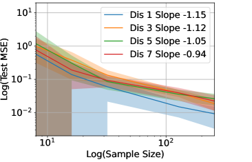
#Λ(f,η)\displaystyle\#\Lambda(f,\eta) =#[Outer leaf nodes of 𝒯(f,η)]\displaystyle=\#\left[\text{Outer leaf nodes of }\mathcal{T}(f,\eta)\right]
22j1+2j2K\displaystyle\leq 2\cdot 2^{j_{1}}+2j_{2}K
22j1+4log2C2ηK\displaystyle\leq 2\cdot 2^{j_{1}}+4\log_{2}\frac{C_{2}}{\eta}K
2(C1η)22r+1+4Klog2C2η\displaystyle\leq 2\left(\frac{C_{1}}{\eta}\right)^{\frac{2}{2r+1}}+4K\log_{2}\frac{C_{2}}{\eta}
6(Cη)22r+1\displaystyle\leq 6\left(\frac{C}{\eta}\right)^{\frac{2}{2r+1}}

when η\eta is sufficiently small, where CC is a constant depending on r,d,Cρ,Kr,d,C_{\rho},K and maxkfr(tk,tk+1)\max_{k}\|f\|_{\mathcal{H}^{r}(t_{k},t_{k+1})}. Notice that

#𝒯(f,η)#Λ(f,η),\#\mathcal{T}(f,\eta)\leq\#\Lambda(f,\eta),

because of (9). Therefore, η22r+1#𝒯(f,η)6C22r+1\eta^{\frac{2}{2r+1}}\#\mathcal{T}(f,\eta)\leq 6C^{\frac{2}{2r+1}} and we have f𝒜r1rf\in\mathcal{A}^{r}_{\lceil r-1\rceil}.

Furthermore, if maxkfr(tk,tk+1)1\max_{k}\|f\|_{\mathcal{H}^{r}(t_{k},t_{k+1})}\leq 1, we have |f|𝒜r1rC(r,d,Cρ,K)|f|_{\mathcal{A}^{r}_{r-1}}\leq C(r,d,C_{\rho},K) for some C(r,d,Cρ,K)C(r,d,C_{\rho},K) depending on r,d,Cρ,Kr,d,C_{\rho},K.

6.4.3 Proof of Example 3a

Proof of Example 3a.

We first estimate δj,k(f)\delta_{j,k}(f) for every cube Cj,kC_{j,k}. There are two types of cubes: the first type belongs to the interior of some Ωt\Omega_{t} and the second type has intersection with some Ωt\partial\Omega_{t} (the boundary of Ωt\Omega_{t}).
The first type (Type I): When Cj,kΩtoC_{j,k}\subset\Omega_{t}^{o} for some tt, we have

δj,k(f)C12j(r+d/2),whereC1=21rCρ12dr/2maxtfr(Ωto)r1!,\delta_{j,k}(f)\leq C_{1}2^{-j(r+d/2)},\ \text{where}\ C_{1}=\frac{2^{1-r}C_{\rho}^{\frac{1}{2}}d^{\lceil r\rceil/2}\max_{t}\|f\|_{\mathcal{H}^{r}(\Omega_{t}^{o})}}{\lceil r-1\rceil!},

according to (67).
The second type (Type II): When Cj,kΩtC_{j,k}\cap\partial\Omega_{t}\neq\emptyset for some tt, ff is irregular on Cj,kC_{j,k}. Similar to (68), we have

δj,kC22jd/2,\displaystyle\delta_{j,k}\leq C_{2}2^{-jd/2},

where C2=2Cρ12fL(Ω)C_{2}=2C_{\rho}^{\frac{1}{2}}\|f\|_{L^{\infty}(\Omega)}.

For any η>0\eta>0, the master tree 𝒯\mathcal{T} is truncated to 𝒯(f,η)\mathcal{T}(f,\eta). Consider the leaf node Cj,k𝒯(f,η)C_{j,k}\in\mathcal{T}(f,\eta). The type-I leaf nodes satisfy 2j>(η/C1)22r+d2^{-j}>(\eta/C_{1})^{\frac{2}{2r+d}}. There are at most 2j1d2^{j_{1}d} leaf nodes of Type I where j1j_{1} is the largest integer with 2j1>(η/C1)22r+d2^{-j_{1}}>(\eta/C_{1})^{\frac{2}{2r+d}}.

We next estimate the number of type-II leaf nodes. The type-II leaf nodes satisfy 2j>(η/C2)2d2^{-j}>\left({\eta}/{C_{2}}\right)^{\frac{2}{d}}. Let j2j_{2} be the largest integer satisfying 2j2>(η/C2)2d2^{-j_{2}}>\left({\eta}/{C_{2}}\right)^{\frac{2}{d}}, which implies j2<2dlog2(Cρ/η)j_{2}<\frac{2}{d}\log_{2}(C_{\rho}/\eta). We next count the number of dyadic cubes needed to cover tΩt\cup_{t}\partial\Omega_{t}, considering tΩt\cup_{t}\partial\Omega_{t} has an upper Minkowski dimension d1d-1. Let cM(tΩt)=supε>0𝒩(ε,tΩt,)εd1c_{M}(\cup_{t}\partial\Omega_{t})=\sup_{\varepsilon>0}\mathcal{N}(\varepsilon,\cup_{t}\Omega_{t},\|\cdot\|_{\infty})\varepsilon^{d-1} be the Minkowski dimension constant of tΩt\cup_{t}\Omega_{t}. According to Definition 2, for each j>0j>0, there exists a collection of SS cubes {Vk}k=1S\{V_{k}\}_{k=1}^{S} of edge length 2j2^{-j} covering tΩt\cup_{t}\partial\Omega_{t} and ScM2j(d1)S\leq c_{M}2^{j(d-1)}. Each VkV_{k} at most intersects with 22d2^{2d} dyadic cubes in the master tree 𝒯\mathcal{T} at scale jj. Therefore, there are at most cM(tΩt)c_{M}(\cup_{t}\partial\Omega_{t}) type-II nodes at scale jj. In total, the number of type-II leaf node is no more than

j=0j22j(d1)+2d=cM(tΩt)22d2j2(d1)2d112d11C¯22d+12j2(d1)\displaystyle\sum_{j=0}^{j_{2}}2^{j(d-1)+2d}=c_{M}(\cup_{t}\partial\Omega_{t})2^{2d}\frac{2^{j_{2}(d-1)}\cdot 2^{d-1}-1}{2^{d-1}-1}\leq\bar{C}2^{2d+1}2^{j_{2}(d-1)} (69)

for some C¯\bar{C} depending on cMc_{M} and dd.

Finally, we count the outer leaf nodes of 𝒯(f,η)\mathcal{T}(f,\eta). The cardinality of the outer leaf nodes of 𝒯(f,η)\mathcal{T}(f,\eta) can be estimated as

#Λ(f,η)\displaystyle\#\Lambda(f,\eta) =#[Outer leaf nodes of 𝒯(f,η)]\displaystyle=\#\left[\text{Outer leaf nodes of }\mathcal{T}(f,\eta)\right]
2d2j1d+2dC¯22d+12j2(d1)\displaystyle\leq 2^{d}\cdot 2^{j_{1}d}+2^{d}\cdot\bar{C}2^{2d+1}2^{j_{2}(d-1)}
<2d(C1η)2d2r+d+2dC¯22d+1(C2η)2(d1)d\displaystyle<2^{d}\left(\frac{C_{1}}{\eta}\right)^{\frac{2d}{2r+d}}+2^{d}\cdot\bar{C}2^{2d+1}\left(\frac{C_{2}}{\eta}\right)^{\frac{2(d-1)}{d}}
C~ηmax{2d2r+d,2(d1)d}\displaystyle\leq\widetilde{C}\eta^{-\max\left\{\frac{2d}{2r+d},\frac{2(d-1)}{d}\right\}}

for some C~\widetilde{C} depending on r,d,cM(tΩt),Cρr,d,c_{M}(\cup_{t}\partial\Omega_{t}),C_{\rho} and maxtfr(Ωto)\max_{t}\|f\|_{\mathcal{H}^{r}(\Omega_{t}^{o})}. Notice that

#𝒯(f,η)#Λ(f,η).\#\mathcal{T}(f,\eta)\leq\#\Lambda(f,\eta).

We have ηmax{2d2r+d,2(d1)d}#𝒯(f,η)C~\eta^{\max\left\{\frac{2d}{2r+d},\frac{2(d-1)}{d}\right\}}\#\mathcal{T}(f,\eta)\leq\widetilde{C}. Thus f𝒜r1sf\in\mathcal{A}^{s}_{\lceil r-1\rceil} with s=min{rd,12(d1)}s=\min\left\{\frac{r}{d},\frac{1}{2(d-1)}\right\}.

Furthermore, if maxtfr(Ωto)1\max_{t}\|f\|_{\mathcal{H}^{r}(\Omega_{t}^{o})}\leq 1, then

|f|𝒜r1sC(r,d,cM(tΩt),Cρ)|f|_{\mathcal{A}^{s}_{\lceil r-1\rceil}}\leq C(r,d,c_{M}(\cup_{t}\partial\Omega_{t}),C_{\rho})

for some C(r,d,cM(tΩt),Cρ)C(r,d,c_{M}(\cup_{t}\partial\Omega_{t}),C_{\rho}) depending on r,d,cM(tΩt)r,d,c_{M}(\cup_{t}\partial\Omega_{t}) and CρC_{\rho}. ∎

6.4.4 Proof of Example 4a

Proof of Example 4a.

We first estimate δj,k(f)\delta_{j,k}(f) for every cube Cj,kC_{j,k}. There are two types of cubes: the first type belongs to Ωδ\Omega_{\delta} and the second type has intersection with Ωδ\Omega^{\complement}_{\delta}.
The first type (Type I): When Cj,kΩδC_{j,k}\subset\Omega_{\delta}, we have

δj,kC12j(r+d/2),\delta_{j,k}\leq C_{1}2^{-j(r+d/2)},

with the C1C_{1} given in (67).
The second type (Type II): When Cj,kΩδC_{j,k}\cap\Omega_{\delta}^{\complement}\neq\emptyset, ff may be irregular on Cj,kC_{j,k} but δj,k=0\delta_{j,k}=0 since Cj,kΩC_{j,k}\subset\Omega^{\complement}, when jj is sufficiently large.

For sufficiently small η>0\eta>0, the master tree 𝒯\mathcal{T} is truncated to 𝒯(f,η)\mathcal{T}(f,\eta). The size of the tree is dominated by the nodes within Ωδ\Omega_{\delta}. Therefore, η22r/d+1#𝒯(f,η)2C2d2r+d\eta^{\frac{2}{2r/d+1}}\#\mathcal{T}(f,\eta)\leq 2C^{\frac{2d}{2r+d}} and f𝒜r1r/df\in\mathcal{A}^{r/d}_{\lceil r-1\rceil}. Furthermore, since CC depends on r,d,Cρr,d,C_{\rho} and fr(Ωδ)\|f\|_{\mathcal{H}^{r}(\Omega_{\delta})}, if fr(Ωδ)1\|f\|_{\mathcal{H}^{r}(\Omega_{\delta})}\leq 1, then |f|𝒜r1r/dC(r,d,Cρ)|f|_{\mathcal{A}^{r/d}_{\lceil r-1\rceil}}\leq C(r,d,C_{\rho}) for some C(r,d,Cρ)C(r,d,C_{\rho}) depending on r,dr,d and CρC_{\rho}.

6.4.5 Proof of Example 5a

Proof of Example 5a.

We first estimate δj,k(f)\delta_{j,k}(f) for every cube Cj,kC_{j,k}. There are two types of cubes: the first type intersects with Ω\Omega and the second type has no intersection with Ω\Omega.
The first type: When IΩI\cap\Omega\neq\emptyset, thanks to (65), we have

δj,k2(f)Cj,kΩ(dr/2fr(X)2(j+1)rr1!)2𝑑ρ=C1222jrρ(Cj,kΩ),\delta_{j,k}^{2}(f)\leq\int_{C_{j,k}\cap\Omega}\left(\frac{d^{\lceil r\rceil/2}\|f\|_{\mathcal{H}^{r}(X)}2^{-(j+1)r}}{\lceil r-1\rceil!}\right)^{2}d\rho=C_{1}^{2}2^{-2jr}\rho(C_{j,k}\cap\Omega),

where C1=dr/2fr(X)2r/r1!.C_{1}={d^{\lceil r\rceil/2}\|f\|_{\mathcal{H}^{r}(X)}2^{-r}}/{\lceil r-1\rceil!}. We next estimate ρ(Cj,kΩ)\rho(C_{j,k}\cap\Omega). Since Ω\Omega is a compact dind_{\rm in}-dimensional Riemannian manifold isometrically embedded in XX, Ω\Omega has a positive reach τ>0\tau>0 (Thäle, 2008, Proposition 14). Each Cj,kC_{j,k} is a dd-dimensional cube of side length 2j2^{-j}, and therefore Cj,kΩC_{j,k}\cap\Omega is contained in an Euclidean ball of diameter d2j.\sqrt{d}2^{-j}. We denote ρΩ\rho_{\Omega} as the conditional measure of ρ\rho on Ω\Omega. According to Maggioni et al. (2016, Lemma 19), when jj is sufficiently small such that d2j<τ/8\sqrt{d}2^{-j}<\tau/8,

ρΩ(Cj,kΩ)(1+(2d2jτ2d2j)2)d2Vol(Bd2j(𝟎din))|Ω|C222jdin,\rho_{\Omega}(C_{j,k}\cap\Omega)\leq\left(1+\left(\frac{2\cdot\sqrt{d}2^{-j}}{\tau-2\cdot\sqrt{d}2^{-j}}\right)^{2}\right)^{\frac{d}{2}}\frac{{\rm Vol}(B_{\sqrt{d}2^{-j}}(\mathbf{0}_{d_{\rm in}}))}{|\Omega|}\leq C_{2}^{2}2^{-j{d_{\rm in}}}, (70)

where Bd2j(𝟎din)B_{\sqrt{d}2^{-j}}(\mathbf{0}_{d_{\rm in}}) denotes the Euclidean ball of radius d2j\sqrt{d}2^{-j} centered at origin in din\mathbb{R}^{d_{\rm in}}, |Ω||\Omega| is the surface area of Ω\Omega, and C2C_{2} is a constant depending on d,τd,\tau and |Ω||\Omega|. (70) implies that

δj,k(f)C1C22j(r+din2).\delta_{j,k}(f)\leq C_{1}C_{2}2^{-j(r+\frac{d_{\rm in}}{2})}.

The second type: When Cj,kΩ=C_{j,k}\cap\Omega=\emptyset, ρX(Cj,k)=0\rho_{X}(C_{j,k})=0 and then δj,k(f)=0.\delta_{j,k}(f)=0.

For any η>0\eta>0, the master tree 𝒯\mathcal{T} is truncated to 𝒯(f,η)\mathcal{T}(f,\eta). The size of the tree is dominated by the nodes intersecting Ω\Omega. The Type-I leaf nodes with δj,k(f)>η\delta_{j,k}(f)>\eta satisfy 2jη22r+din2^{-j}\gtrsim\eta^{\frac{2}{2r+d_{\rm in}}}. At scale jj, there are at most O(2jdin)O(2^{jd_{\rm in}}) Type-I leaf nodes. The cardinality of 𝒯(f,η)\mathcal{T}(f,\eta) satisfies

#𝒯(f,η)\displaystyle\#\mathcal{T}(f,\eta) η2din2r+din.\displaystyle\lesssim\eta^{-\frac{2d_{\rm in}}{2r+d_{\rm in}}}.

Therefore, supη>0η2din2r+din#𝒯(f,η)<\sup_{\eta>0}\eta^{\frac{2{d_{\rm in}}}{2r+{d_{\rm in}}}}\#\mathcal{T}(f,\eta)<\infty, so that f𝒜r1r/dinf\in\mathcal{A}^{r/{d_{\rm in}}}_{\lceil r-1\rceil}. Furthermore, if fr(X)1\|f\|_{\mathcal{H}^{r}(X)}\leq 1, we have |f|𝒜r1r/din<C(r,d,din,τ,|Ω|)|f|_{\mathcal{A}^{r/d_{\rm in}}_{\lceil r-1\rceil}}<C(r,d,d_{\rm in},\tau,|\Omega|) with C(r,d,din,τ,|Ω|)C(r,d,d_{\rm in},\tau,|\Omega|) depending on r,d,din,τr,d,d_{\rm in},\tau and |Ω||\Omega|.

7 Conclusion

In this paper, we establish approximation and generalization theories for a large function class which is defined by nonlinear tree-based approximation theory. Such a function class allows the regularity of the function to vary at different locations and scales. It covers common function classes, such as Hölder functions and discontinuous functions, such as piecewise Hölder functions. Our theory shows that deep neural networks are adaptive to nonuniform regularity of functions and data distributions at different locations and scales.

When deep learning is used for regression, different network architectures can give rise to very different results. The success of deep learning relies on the optimization algorithm, initialization and a proper choice of network architecture. We will leave the computational study as our future research.

Appendix

Appendix A Proof of the approximation error in (10)

The approximation error in (10) can be proved as follows:

fpΛ(f,η)L2(ρ)2\displaystyle\|f-p_{\Lambda(f,\eta)}\|_{L^{2}(\rho)}^{2} =Cj,k𝒯(f,η)ψj,k(f)L2(ρ)2=0Cj,k𝒯(f,2(+1)η)𝒯(f,2η)ψj,k(f)L2(ρ)2\displaystyle=\sum_{C_{j,k}\notin\mathcal{T}(f,\eta)}\|\psi_{j,k}(f)\|_{L^{2}(\rho)}^{2}=\sum_{\ell\geq 0}\sum_{C_{j,k}\in\mathcal{T}(f,2^{-(\ell+1)}\eta)\setminus\mathcal{T}(f,2^{-\ell}\eta)}\|\psi_{j,k}(f)\|_{L^{2}(\rho)}^{2}
0(2η)2#[𝒯(f,2(+1)η)]0(2η)2|f|𝒜θsm[2(+1)η]m\displaystyle\leq\sum_{\ell\geq 0}(2^{-\ell}\eta)^{2}\#[\mathcal{T}(f,2^{-(\ell+1)}\eta)]\leq\sum_{\ell\geq 0}(2^{-\ell}\eta)^{2}|f|_{\mathcal{A}^{s}_{\theta}}^{m}[2^{-(\ell+1)}\eta]^{-m}
=[2m02(m2)]|f|𝒜θsmη2m=Cs|f|𝒜θsmη2mCs|f|𝒜θs2(#𝒯(f,η))2s\displaystyle=[2^{m}\sum_{\ell\geq 0}2^{\ell(m-2)}]|f|_{\mathcal{A}^{s}_{\theta}}^{m}\eta^{2-m}=C_{s}|f|_{\mathcal{A}^{s}_{\theta}}^{m}\eta^{2-m}\leq C_{s}|f|_{\mathcal{A}^{s}_{\theta}}^{2}(\#\mathcal{T}(f,\eta))^{-{2s}}

since η2m|f|𝒜θs2m(#𝒯(f,η))2mm=|f|𝒜θs2m(#𝒯(f,η))2s\eta^{2-m}\leq|f|_{\mathcal{A}^{s}_{\theta}}^{2-m}(\#\mathcal{T}(f,\eta))^{-\frac{2-m}{m}}=|f|_{\mathcal{A}^{s}_{\theta}}^{2-m}(\#\mathcal{T}(f,\eta))^{-{2s}} by the definition in (8).

Appendix B Proof of Lemma 1

Proof of Lemma 1.

Let ={𝐱𝜶:|𝜶|=α1++αdθ}\mathcal{R}=\{\mathbf{x}^{\bm{\alpha}}:|\bm{\alpha}|=\alpha_{1}+\ldots+\alpha_{d}\leq\theta\}, and np=#n_{p}=\#\mathcal{R} be the cardinality of \mathcal{R}. Denote Ω~=[0,1]d\widetilde{\Omega}=[0,1]^{d}. We first index the elements in \mathcal{R} according to |𝜶||\bm{\alpha}| in the non-decreasing order. One can obtain a set of orthonormal polynomials on Ω~\widetilde{\Omega} from \mathcal{R} by the Gram–Schmidt process. This set of polynomials forms an orthonormal basis for polynomials on Ω~\widetilde{\Omega} with degree no more than θ\theta. Denote this orthonormal set of polynomials by {ϕ~}=1np\{\widetilde{\phi}_{\ell}\}_{\ell=1}^{n_{p}}. Each ϕ~\widetilde{\phi}_{\ell} can be written as

ϕ~(𝐱)=|𝜶|θb~,𝜶𝐱𝜶\displaystyle\widetilde{\phi}_{\ell}(\mathbf{x})=\sum_{|\bm{\alpha}|\leq\theta}\widetilde{b}_{\ell,\bm{\alpha}}\mathbf{x}^{\bm{\alpha}} (71)

for some {b~,𝜶}𝜶\{\widetilde{b}_{\ell,\bm{\alpha}}\}_{\bm{\alpha}}. There exists a constant C1C_{1} only depending on θ\theta and dd so that

|b~,𝜶|C1=1,,np and |𝜶|θ.\displaystyle|\widetilde{b}_{\ell,\bm{\alpha}}|\leq C_{1}\quad\forall\ell=1,...,n_{p}\mbox{ and }|\bm{\alpha}|\leq\theta. (72)

For the simplicity of notation, we denote Ω=Cj,k=[𝐚,𝒃]\Omega=C_{j,k}=[\mathbf{a},\bm{b}] with 𝐚=[a1,,ad],𝒃=[b1,,bd]\mathbf{a}=[a_{1},...,a_{d}],\bm{b}=[b_{1},...,b_{d}] and b1a1==bdad=h=2jb_{1}-a_{1}=\cdots=b_{d}-a_{d}=h=2^{-j}. The idea of this proof is to obtain a set of orthonormal basis on Ω\Omega from (71), where each basis is a linear combination of monomials of (𝐱𝐚h)\left(\frac{\mathbf{x}-\mathbf{a}}{h}\right). Then the coefficients of pj,kp_{j,k} can be expressed as inner product between ff and each basis. Let

ϕ(𝐱)=1hd/2ϕ~(𝐱𝐚h).\displaystyle\phi_{\ell}(\mathbf{x})=\frac{1}{h^{d/2}}\widetilde{\phi}_{\ell}\left(\frac{\mathbf{x}-\mathbf{a}}{h}\right). (73)

The ϕ\phi_{\ell}’s form a set of orthonormal polynomials on Ω\Omega, since

ϕ1,ϕ2\displaystyle\langle\phi_{\ell_{1}},\phi_{\ell_{2}}\rangle
=\displaystyle= Ωϕ1(𝐱)ϕ2(𝐱)𝑑𝐱\displaystyle\int_{\Omega}\phi_{\ell_{1}}(\mathbf{x})\phi_{\ell_{2}}(\mathbf{x})d\mathbf{x}
=\displaystyle= 1hdΩϕ~1((𝐱𝐚h))ϕ~2((𝐱𝐚h))𝑑𝐱\displaystyle\frac{1}{h^{d}}\int_{\Omega}\widetilde{\phi}_{\ell_{1}}\left(\left(\frac{\mathbf{x}-\mathbf{a}}{h}\right)\right)\widetilde{\phi}_{\ell_{2}}\left(\left(\frac{\mathbf{x}-\mathbf{a}}{h}\right)\right)d\mathbf{x}
=\displaystyle= hdhdΩϕ~1((𝐱𝐚h))ϕ~2((𝐱𝐚h))d(𝐱𝐚h)\displaystyle\frac{h^{d}}{h^{d}}\int_{\Omega}\widetilde{\phi}_{\ell_{1}}\left(\left(\frac{\mathbf{x}-\mathbf{a}}{h}\right)\right)\widetilde{\phi}_{\ell_{2}}\left(\left(\frac{\mathbf{x}-\mathbf{a}}{h}\right)\right)d\left(\frac{\mathbf{x}-\mathbf{a}}{h}\right)
=\displaystyle= Ω~ϕ~1(𝐱)ϕ~2(𝐱)𝑑𝐱\displaystyle\int_{\widetilde{\Omega}}\widetilde{\phi}_{\ell_{1}}\left(\mathbf{x}\right)\widetilde{\phi}_{\ell_{2}}\left(\mathbf{x}\right)d\mathbf{x}
=\displaystyle= {1 if 1=2,0 otherwise.\displaystyle\begin{cases}1\mbox{ if }\ell_{1}=\ell_{2},\\ 0\mbox{ otherwise}.\end{cases}

Thus {ϕ}=1np\{\phi_{\ell}\}_{\ell=1}^{n_{p}} form an orthonormal basis for polynomials with degree no more than θ\theta on Ω\Omega. The pj,kp_{j,k} in (4) has the form

pj,k==1npcϕ with c=Ωf(𝐱)ϕ(𝐱)𝑑𝐱.\displaystyle p_{j,k}=\sum_{\ell=1}^{n_{p}}c_{\ell}\phi_{\ell}\quad\mbox{ with }\quad c_{\ell}=\int_{\Omega}f(\mathbf{x})\phi_{\ell}(\mathbf{x})d\mathbf{x}. (74)

Using Hölder’s inequality, we have

|c|=|f,ϕ|fL2(Ω)ϕL2(Ω)R|Ω|Rhd/2.\displaystyle|c_{\ell}|=\left|\langle f,\phi_{\ell}\rangle\right|\leq\|f\|_{L^{2}(\Omega)}\|\phi_{\ell}\|_{L^{2}(\Omega)}\leq R\sqrt{|\Omega|}\leq Rh^{d/2}. (75)

Substituting (73) and (71) into (74) gives rise to

pj,k(𝐱)==1npck|𝜶|θb~k,𝜶hd/2(𝐱𝐚h)𝜶=|𝜶|θ(=1npcb~,𝜶hd/2)(𝐱𝐚h)𝜶,\displaystyle p_{j,k}(\mathbf{x})=\sum_{\ell=1}^{n_{p}}c_{k}\sum_{|\bm{\alpha}|\leq\theta}\frac{\widetilde{b}_{k,\bm{\alpha}}}{h^{d/2}}\left(\frac{\mathbf{x}-\mathbf{a}}{h}\right)^{\bm{\alpha}}=\sum_{|\bm{\alpha}|\leq\theta}\left(\sum_{\ell=1}^{n_{p}}\frac{c_{\ell}\widetilde{b}_{\ell,\bm{\alpha}}}{h^{d/2}}\right)\left(\frac{\mathbf{x}-\mathbf{a}}{h}\right)^{\bm{\alpha}},

implying that

a𝜶==1npcb~,𝜶hd/2.a_{\bm{\alpha}}=\sum_{\ell=1}^{n_{p}}\frac{c_{\ell}\widetilde{b}_{\ell,\bm{\alpha}}}{h^{d/2}}.

Putting (72) and (75) together, we have

|a𝜶|k=1np|ck||b~k,𝜶|hd/2k=1npC1Rhd/2hd/2=C1npR,\displaystyle|a_{\bm{\alpha}}|\leq\sum_{k=1}^{n_{p}}\frac{|c_{k}||\widetilde{b}_{k,\bm{\alpha}}|}{h^{d/2}}\leq\sum_{k=1}^{n_{p}}\frac{C_{1}Rh^{d/2}}{h^{d/2}}=C_{1}n_{p}R, (76)

where C1C_{1}, as defined in (72), is a constant depending on θ\theta.

Furthermore, since (𝐱𝐚h)𝜶1\|\left(\frac{\mathbf{x}-\mathbf{a}}{h}\right)^{\bm{\alpha}}\|_{\infty}\leq 1, we have

pj,kL(Ω)C1np2R.\displaystyle\|p_{j,k}\|_{L^{\infty}(\Omega)}\leq C_{1}n_{p}^{2}R.

Appendix C Proof of Lemma 3

Proof of Lemma 3.

Denote the product ×(a,b)=a×b\times(a,b)=a\times b. Let ×~(,)\widetilde{\times}(\cdot,\cdot) be the network specified in Lemma 3 with accuracy ε\varepsilon. We construct

Π~(a1,,aN)=×~(a1,×~(a2,×~(,×~(aN1,aN))))\displaystyle\widetilde{\Pi}(a_{1},...,a_{N})=\widetilde{\times}(a_{1},\widetilde{\times}(a_{2},\widetilde{\times}(\cdots,\widetilde{\times}(a_{N-1},a_{N})\cdots))) (77)

to approximate the multiplication operation i=1Nai=a1×a2××aN\prod_{i=1}^{N}a_{i}=a_{1}\times a_{2}\times\cdots\times a_{N}. The approximation error can be bounded as

|Π~(a1,,aN)i=1Nai|\displaystyle|\widetilde{\Pi}(a_{1},...,a_{N})-\prod_{i=1}^{N}a_{i}|
=\displaystyle= |×~(a1,×~(a2,×~(,×~(aN1,aN))))×(a1,×(a2,×(,×(aN1,aN))))|\displaystyle|\widetilde{\times}(a_{1},\widetilde{\times}(a_{2},\widetilde{\times}(\cdots,\widetilde{\times}(a_{N-1},a_{N})\cdots)))-\times(a_{1},\times(a_{2},\times(\cdots,\times(a_{N-1},a_{N})\cdots)))|
\displaystyle\leq |×~(a1,×~(a2,×~(,×~(aN1,aN))))×(a1,×~(a2,×~(,×~(aN1,aN))))|\displaystyle|\widetilde{\times}(a_{1},\widetilde{\times}(a_{2},\widetilde{\times}(\cdots,\widetilde{\times}(a_{N-1},a_{N})\cdots)))-\times(a_{1},\widetilde{\times}(a_{2},\widetilde{\times}(\cdots,\widetilde{\times}(a_{N-1},a_{N})\cdots)))|
+|×(a1,×~(a2,×~(,×~(aN1,aN))))×(a1,×(a2,×~(,×~(aN1,aN))))|\displaystyle+|\times(a_{1},\widetilde{\times}(a_{2},\widetilde{\times}(\cdots,\widetilde{\times}(a_{N-1},a_{N})\cdots)))-\times(a_{1},\times(a_{2},\widetilde{\times}(\cdots,\widetilde{\times}(a_{N-1},a_{N})\cdots)))|
+\displaystyle+\cdots
+|×(a1,×(a2,×(,×~(aN1,aN))))×(a1,×(a2,×(,×(aN1,aN))))|\displaystyle+|\times(a_{1},\times(a_{2},\times(\cdots,\widetilde{\times}(a_{N-1},a_{N})\cdots)))-\times(a_{1},\times(a_{2},\times(\cdots,\times(a_{N-1},a_{N})\cdots)))|
\displaystyle\leq Nε.\displaystyle N\varepsilon. (78)

The network size is specified in (27). ∎

Appendix D Proof of Lemma 4

Proof of Lemma 4.

Let jj^{*} be the smallest integer so that 2dj#Λ𝒯2^{dj^{*}}\geq\#\Lambda_{{\mathcal{T}}}. Based on 𝒯{\mathcal{T}}, we first construct a 𝒯{\mathcal{T}}^{\prime} so that #Λ𝒯=#Λ𝒯\#\Lambda_{{\mathcal{T}}^{\prime}}=\#\Lambda_{{\mathcal{T}}} and jjj\leq j^{*} for any Cj,kΛ𝒯C_{j,k}\in\Lambda_{{\mathcal{T}}^{\prime}} by the following procedure.

Note that if there exists Cj1,kΛ𝒯C_{j_{1},k}\in\Lambda_{{\mathcal{T}}} with j1>jj_{1}>j^{*}, there must be a Cj2,kΛ𝒯C_{j_{2},k^{\prime}}\in\Lambda_{{\mathcal{T}}} with j2<jj_{2}<j^{*}. Otherwise, we must have #Λ𝒯>2dj\#\Lambda_{{\mathcal{T}}}>2^{dj^{*}}, contradicting to the definition of jj^{*}. Let Cj1,kC_{j_{1},k} be a subcube in the finest scale of Λ𝒯\Lambda_{{\mathcal{T}}}, and Cj2,kC_{j_{2},k^{\prime}} be a subcube in the coarsest scale of Λ𝒯\Lambda_{{\mathcal{T}}}. Suppose j1>jj_{1}>j^{*}. We have j1j22j_{1}-j_{2}\geq 2. Denote the set of children and the parent of Cj,kC_{j,k} by 𝒞(Cj,k)\mathcal{C}(C_{j,k}) and 𝒫(Cj,k)\mathcal{P}(C_{j,k}), respectively. Since Cj1,kC_{j_{1},k} is at the finest scale, we have 𝒞(𝒫(Cj1,k))Λ𝒯\mathcal{C}(\mathcal{P}(C_{j_{1},k}))\subset\Lambda_{{\mathcal{T}}}. By replacing 𝒞(𝒫(Cj1,k))\mathcal{C}(\mathcal{P}(C_{j_{1},k})) by 𝒫(Cj1,k)\mathcal{P}(C_{j_{1},k}) and Cj2,kC_{j_{2},k^{\prime}} by 𝒞(Cj2,k)\mathcal{C}(C_{j_{2},k^{\prime}}), we obtain a new tree 𝒯1{\mathcal{T}}_{1} with #Λ𝒯1=#Λ𝒯2dj\#\Lambda_{{\mathcal{T}}_{1}}=\#\Lambda_{{\mathcal{T}}}\leq 2^{dj^{*}}. Note that the subcubes in 𝒞(𝒫(Cj1,k))\mathcal{C}(\mathcal{P}(C_{j_{1},k})) have side length 2j12^{-j_{1}}, Cj2,kC_{j_{2},k^{\prime}} has side length 2j22^{-j_{2}}. Since j1j22j_{1}-j_{2}\geq 2, we have

|(Λ𝒯1)||(Λ𝒯)|=d2j2(d1)d2j1(d1)>0,\displaystyle|\mathcal{B}(\Lambda_{{\mathcal{T}}_{1}})|-|\mathcal{B}(\Lambda_{{\mathcal{T}}})|=d2^{-j_{2}(d-1)}-d2^{-j_{1}(d-1)}>0, (79)

implying that |(Λ𝒯)|<|(Λ𝒯1)||\mathcal{B}(\Lambda_{{\mathcal{T}}})|<|\mathcal{B}(\Lambda_{{\mathcal{T}}_{1}})|. Replace 𝒯{\mathcal{T}} by 𝒯1{\mathcal{T}}_{1} and repeat the above procedure, we can generate a set of trees {𝒯m}m=1M\{{\mathcal{T}}_{m}\}_{m=1}^{M} for some M>0M>0 until jjj\leq j^{*} for all Cj,kΛ𝒯MC_{j,k}\in\Lambda_{{\mathcal{T}}_{M}}. We have

|(Λ𝒯)|<|(Λ𝒯1)|<<|(Λ𝒯M)|.|\mathcal{B}(\Lambda_{{\mathcal{T}}})|<|\mathcal{B}(\Lambda_{{\mathcal{T}}_{1}})|<\cdots<|\mathcal{B}(\Lambda_{{\mathcal{T}}_{M}})|.

All leaf nodes of 𝒯M{\mathcal{T}}_{M} are at scale no larger than j1j^{*}-1. For any leaf node Cj,kC_{j,k} of 𝒯M{\mathcal{T}}_{M} with j<j1j<j^{*}-1, we partition it into its children. Repeat this process until all leaf nodes of the tree is at scale j1j^{*}-1, and denote the tree by 𝒯{\mathcal{T}}^{*}. Note that doing so only creates additional common boundaries, thus (Λ𝒯M)(Λ𝒯)\mathcal{B}(\Lambda_{{\mathcal{T}}_{M}})\subset\mathcal{B}(\Lambda_{{\mathcal{T}}^{*}}), and we have

|(Λ𝒯)|<|(Λ𝒯M)|<|(Λ𝒯)|.|\mathcal{B}(\Lambda_{{\mathcal{T}}})|<|\mathcal{B}(\Lambda_{{\mathcal{T}}_{M}})|<|\mathcal{B}(\Lambda_{{\mathcal{T}}^{*}})|.

We next compute |(Λ𝒯)||\mathcal{B}(\Lambda_{{\mathcal{T}}^{*}})|. Note that (Λ𝒯)\mathcal{B}(\Lambda_{{\mathcal{T}}^{*}}) can be generated sequentially by slicing each cube at scale jj for j=0,,j1j=0,...,j^{*}-1. When Cj1,kC_{j-1,k} is sliced to get cubes at scale jj, dd hyper-surfaces with area 2(j1)(d1)2^{-(j-1)(d-1)} are created as common boundaries. There are in total 2d(j1)2^{d(j-1)} cubes at scale jj. Thus we compute |(Λ𝒯)||\mathcal{B}(\Lambda_{{\mathcal{T}}^{*}})| as:

|(Λ𝒯)|=j=1jd2(j1)(d1)2d(j1)=j=1jd2j1=d(2j1)d2j2dd(#Λ𝒯)1/d2d+1d(#𝒯)1/d,\displaystyle|\mathcal{B}(\Lambda_{{\mathcal{T}}^{*}})|=\sum_{j=1}^{j^{*}}d2^{-(j-1)(d-1)}2^{d(j-1)}=\sum_{j=1}^{j^{*}}d2^{j-1}=d(2^{j^{*}}-1)\leq d2^{j^{*}}\leq 2^{d}d(\#\Lambda_{{\mathcal{T}}})^{1/d}\leq 2^{d+1}d(\#{\mathcal{T}})^{1/d}, (80)

where we used #Λ𝒯2dj2d#Λ𝒯\#\Lambda_{{\mathcal{T}}}\leq 2^{dj^{*}}\leq 2^{d}\#\Lambda_{{\mathcal{T}}} in the second inequality according to the definition of jj^{*}. ∎

Appendix E Proof of Lemma 5

Proof of Lemma 5.

Let ={fNN,j}j=1𝒩(δ,,L(X))\mathcal{F}^{*}=\left\{f_{{\rm NN},j}\right\}_{j=1}^{\mathcal{N}(\delta,\mathcal{F},\|\cdot\|_{L^{\infty}(X)})} be a δ\delta cover of \mathcal{F}. There exists fNNf_{\rm NN}^{*}\in\mathcal{F}^{*} satisfying fNNf^L(X)δ\|f_{\rm NN}^{*}-\widehat{f}\|_{L^{\infty}(X)}\leq\delta.

We have

𝔼𝒮[1ni=1nξif^(𝐱i))]=\displaystyle\mathbb{E}_{{\mathcal{S}}}\left[\frac{1}{n}\sum_{i=1}^{n}\xi_{i}\widehat{f}(\mathbf{x}_{i}))\right]= 𝔼𝒮[1ni=1nξi(f^(𝐱i)fNN(𝐱i)+fNN(𝐱i)f(𝐱i))]\displaystyle\mathbb{E}_{{\mathcal{S}}}\left[\frac{1}{n}\sum_{i=1}^{n}\xi_{i}(\widehat{f}(\mathbf{x}_{i})-f_{\rm NN}^{*}(\mathbf{x}_{i})+f_{\rm NN}^{*}(\mathbf{x}_{i})-f(\mathbf{x}_{i}))\right]
\displaystyle\leq 𝔼𝒮[1ni=1nξi(fNN(𝐱i)f(𝐱i))]+𝔼𝒮[1ni=1n|ξi||f^(𝐱i)fNN(𝐱i)|]\displaystyle\mathbb{E}_{{\mathcal{S}}}\left[\frac{1}{n}\sum_{i=1}^{n}\xi_{i}(f_{\rm NN}^{*}(\mathbf{x}_{i})-f(\mathbf{x}_{i}))\right]+\mathbb{E}_{{\mathcal{S}}}\left[\frac{1}{n}\sum_{i=1}^{n}|\xi_{i}|\left|\widehat{f}(\mathbf{x}_{i})-f_{\rm NN}^{*}(\mathbf{x}_{i})\right|\right]
\displaystyle\leq 𝔼𝒮[fNNfnni=1nξi(fNN(𝐱i)fNN(𝐱i))nfNNfn]+δσ\displaystyle\mathbb{E}_{{\mathcal{S}}}\left[\frac{\|f_{\rm NN}^{*}-f\|_{n}}{\sqrt{n}}\frac{\sum_{i=1}^{n}\xi_{i}\left(f_{\rm NN}^{*}(\mathbf{x}_{i})-f_{\rm NN}^{*}(\mathbf{x}_{i})\right)}{\sqrt{n}\|f_{\rm NN}^{*}-f\|_{n}}\right]+\delta\sigma
\displaystyle\leq 2𝔼𝒮[f^fn+δn|i=1nξi(fNN(𝐱i)fNN(𝐱i))nfNNfn|]+δσ.\displaystyle\sqrt{2}\mathbb{E}_{{\mathcal{S}}}\left[\frac{\|\widehat{f}-f\|_{n}+\delta}{\sqrt{n}}\left|\frac{\sum_{i=1}^{n}\xi_{i}\left(f_{\rm NN}^{*}(\mathbf{x}_{i})-f_{\rm NN}^{*}(\mathbf{x}_{i})\right)}{\sqrt{n}\|f_{\rm NN}^{*}-f\|_{n}}\right|\right]+\delta\sigma. (81)

In (81), the first inequality follows from Cauchy-Schwarz inequality, the second inequality holds by Jensen’s inequality and

𝔼𝒮[1ni=1n|ξi||f^(𝐱i)fNN(𝐱i)|]\displaystyle\mathbb{E}_{{\mathcal{S}}}\left[\frac{1}{n}\sum_{i=1}^{n}|\xi_{i}|\left|\widehat{f}(\mathbf{x}_{i})-f_{\rm NN}^{*}(\mathbf{x}_{i})\right|\right]\leq 𝔼𝒮[1ni=1n|ξi|f^(𝐱i)fNN(𝐱i)L(X)]\displaystyle\mathbb{E}_{{\mathcal{S}}}\left[\frac{1}{n}\sum_{i=1}^{n}|\xi_{i}|\left\|\widehat{f}(\mathbf{x}_{i})-f_{\rm NN}^{*}(\mathbf{x}_{i})\right\|_{L^{\infty}(X)}\right]
\displaystyle\leq δ1ni=1n𝔼𝒮[ξi2]\displaystyle\delta\frac{1}{n}\sum_{i=1}^{n}\mathbb{E}_{{\mathcal{S}}}\left[\sqrt{\xi_{i}^{2}}\right]
\displaystyle\leq δ1ni=1n𝔼𝒮[ξi2]\displaystyle\delta\frac{1}{n}\sum_{i=1}^{n}\sqrt{\mathbb{E}_{{\mathcal{S}}}\left[\xi_{i}^{2}\right]}
\displaystyle\leq δ1ni=1nσ2\displaystyle\delta\frac{1}{n}\sum_{i=1}^{n}\sqrt{\sigma^{2}}
=\displaystyle= δσ,\displaystyle\delta\sigma, (82)

the last inequality holds since

fNNfn=\displaystyle\|f_{\rm NN}^{*}-f\|_{n}= 1ni=1n(fNN(𝐱i)f^(𝐱i)+f^(𝐱i)f(𝐱i))2\displaystyle\sqrt{\frac{1}{n}\sum_{i=1}^{n}(f_{\rm NN}^{*}(\mathbf{x}_{i})-\widehat{f}(\mathbf{x}_{i})+\widehat{f}(\mathbf{x}_{i})-f(\mathbf{x}_{i}))^{2}}
\displaystyle\leq 2ni=1n[(fNN(𝐱i)f^(𝐱i))2+(f^(𝐱i)f(𝐱i))2]\displaystyle\sqrt{\frac{2}{n}\sum_{i=1}^{n}\left[(f_{\rm NN}^{*}(\mathbf{x}_{i})-\widehat{f}(\mathbf{x}_{i}))^{2}+(\widehat{f}(\mathbf{x}_{i})-f(\mathbf{x}_{i}))^{2}\right]}
\displaystyle\leq 2ni=1n[δ2+(f^(𝐱i)f(𝐱i))2]\displaystyle\sqrt{\frac{2}{n}\sum_{i=1}^{n}\left[\delta^{2}+(\widehat{f}(\mathbf{x}_{i})-f(\mathbf{x}_{i}))^{2}\right]}
\displaystyle\leq 2f^fn+2δ.\displaystyle\sqrt{2}\|\widehat{f}-f\|_{n}+\sqrt{2}\delta. (83)

Denote zj=i=1nξi(f^(𝐱i)fNN(𝐱i))nfNNfnz_{j}=\frac{\sum_{i=1}^{n}\xi_{i}(\widehat{f}(\mathbf{x}_{i})-f_{\rm NN}^{*}(\mathbf{x}_{i}))}{\sqrt{n}\|f_{\rm NN}^{*}-f\|_{n}}. The first term in (81) can be bounded as

2𝔼𝒮[f^fn+δn|i=1nξi(f^(𝐱i)fNN(𝐱i))nfNNfn|]\displaystyle\sqrt{2}\mathbb{E}_{{\mathcal{S}}}\left[\frac{\|\widehat{f}-f\|_{n}+\delta}{\sqrt{n}}\left|\frac{\sum_{i=1}^{n}\xi_{i}(\widehat{f}(\mathbf{x}_{i})-f_{\rm NN}^{*}(\mathbf{x}_{i}))}{\sqrt{n}\|f_{\rm NN}^{*}-f\|_{n}}\right|\right]
\displaystyle\leq 2𝔼𝒮[f^fn+δnmaxj|zj|]\displaystyle\sqrt{2}\mathbb{E}_{{\mathcal{S}}}\left[\frac{\|\widehat{f}-f\|_{n}+\delta}{\sqrt{n}}\max_{j}|z_{j}|\right]
=\displaystyle= 2𝔼𝒮[f^fnnmaxj|zj|+δnmaxj|zj|]\displaystyle\sqrt{2}\mathbb{E}_{{\mathcal{S}}}\left[\frac{\|\widehat{f}-f\|_{n}}{\sqrt{n}}\max_{j}|z_{j}|+\frac{\delta}{\sqrt{n}}\max_{j}|z_{j}|\right]
=\displaystyle= 2𝔼𝒮[1nf^fn2maxj|zj|2+δnmaxj|zj|2]\displaystyle\sqrt{2}\mathbb{E}_{{\mathcal{S}}}\left[\sqrt{\frac{1}{n}\|\widehat{f}-f\|_{n}^{2}}\sqrt{\max_{j}|z_{j}|^{2}}+\frac{\delta}{\sqrt{n}}\sqrt{\max_{j}|z_{j}|^{2}}\right]
\displaystyle\leq 21n𝔼𝒮[f^fn2]𝔼𝒮[maxj|zj|2]+δn𝔼𝒮[maxj|zj|2]\displaystyle\sqrt{2}\sqrt{\frac{1}{n}\mathbb{E}_{{\mathcal{S}}}\left[\|\widehat{f}-f\|_{n}^{2}\right]}\sqrt{\mathbb{E}_{{\mathcal{S}}}\left[\max_{j}|z_{j}|^{2}\right]}+\frac{\delta}{\sqrt{n}}\sqrt{\mathbb{E}_{{\mathcal{S}}}\left[\max_{j}|z_{j}|^{2}\right]}
=\displaystyle= 2(1n𝔼𝒮[f^fn2]+δn)𝔼𝒮[maxj|zj|2],\displaystyle\sqrt{2}\left(\sqrt{\frac{1}{n}\mathbb{E}_{{\mathcal{S}}}\left[\|\widehat{f}-f\|_{n}^{2}\right]}+\frac{\delta}{\sqrt{n}}\right)\sqrt{\mathbb{E}_{{\mathcal{S}}}\left[\max_{j}|z_{j}|^{2}\right]}, (84)

where the second inequality comes from Jensen’s inequality and Cauchy-Schwarz inequality.

For given {𝐱i}i=1n\{\mathbf{x}_{i}\}_{i=1}^{n}, zjz_{j} is a sub-Gaussian variable with variance proxy σ2\sigma^{2}.

For any t>0t>0, we have

𝔼𝒮[maxj|zj|2|𝐱1,,𝐱n]=\displaystyle\mathbb{E}_{{\mathcal{S}}}\left[\max_{j}|z_{j}|^{2}|\mathbf{x}_{1},...,\mathbf{x}_{n}\right]= 1tlogexp(t𝔼𝒮[maxj|zj|2|𝐱1,,𝐱n])\displaystyle\frac{1}{t}\log\exp\left(t\mathbb{E}_{{\mathcal{S}}}\left[\max_{j}|z_{j}|^{2}|\mathbf{x}_{1},...,\mathbf{x}_{n}\right]\right)
\displaystyle\leq 1tlog𝔼𝒮[exp(tmaxj|zj|2)|𝐱1,,𝐱n]\displaystyle\frac{1}{t}\log\mathbb{E}_{{\mathcal{S}}}\left[\exp\left(t\max_{j}|z_{j}|^{2}\right)|\mathbf{x}_{1},...,\mathbf{x}_{n}\right]
\displaystyle\leq 1tlog𝔼𝒮[jexp(t|zj|2)|𝐱1,,𝐱n]\displaystyle\frac{1}{t}\log\mathbb{E}_{{\mathcal{S}}}\left[\sum_{j}\exp\left(t|z_{j}|^{2}\right)|\mathbf{x}_{1},...,\mathbf{x}_{n}\right]
\displaystyle\leq 1tlog𝒩(δ,,L(X))+1tlog𝔼𝒮[exp(t|z1|2)|𝐱1,,𝐱n].\displaystyle\frac{1}{t}\log\mathcal{N}(\delta,\mathcal{F},\|\cdot\|_{L^{\infty}(X)})+\frac{1}{t}\log\mathbb{E}_{{\mathcal{S}}}\left[\exp(t|z_{1}|^{2}\right)|\mathbf{x}_{1},...,\mathbf{x}_{n}]. (85)

Since z1z_{1} is a sub-Gaussian variable with parameter σ\sigma, we have

𝔼𝒮[exp(t|z1|2)|𝐱1,,𝐱n]=\displaystyle\mathbb{E}_{{\mathcal{S}}}\left[\exp(t|z_{1}|^{2})|\mathbf{x}_{1},...,\mathbf{x}_{n}\right]= 1+k=1tk𝔼𝒮[z12k|𝐱1,,𝐱n]k!\displaystyle 1+\sum_{k=1}^{\infty}\frac{t^{k}\mathbb{E}_{{\mathcal{S}}}\left[z_{1}^{2k}|\mathbf{x}_{1},...,\mathbf{x}_{n}\right]}{k!}
=\displaystyle= 1+k=1tkk!0(|z1|λ12k|𝐱1,,𝐱n)𝑑λ\displaystyle 1+\sum_{k=1}^{\infty}\frac{t^{k}}{k!}\int_{0}^{\infty}\mathbb{P}\left(|z_{1}|\geq\lambda^{\frac{1}{2k}}|\mathbf{x}_{1},...,\mathbf{x}_{n}\right)d\lambda
\displaystyle\leq 1+2k=1tkk!0exp(λ1/k2σ2)𝑑λ\displaystyle 1+2\sum_{k=1}^{\infty}\frac{t^{k}}{k!}\int_{0}^{\infty}\exp\left(-\frac{\lambda^{1/k}}{2\sigma^{2}}\right)d\lambda
=\displaystyle= 1+k=12k(2tσ2)kk!ΓG(k)\displaystyle 1+\sum_{k=1}^{\infty}\frac{2k(2t\sigma^{2})^{k}}{k!}\Gamma_{G}(k)
=\displaystyle= 1+2k=1(2tσ2)k,\displaystyle 1+2\sum_{k=1}^{\infty}(2t\sigma^{2})^{k}, (86)

where ΓG\Gamma_{G} represents the Gamma function. Set t=(4σ2)1t=(4\sigma^{2})^{-1}, we have

𝔼𝒮[maxj|zj|2|𝐱1,,𝐱n]4σ2log𝒩(δ,,L(X))+4σ2log34σ2log𝒩(δ,,L(X))+6σ2.\displaystyle\mathbb{E}_{{\mathcal{S}}}\left[\max_{j}|z_{j}|^{2}|\mathbf{x}_{1},...,\mathbf{x}_{n}\right]\leq 4\sigma^{2}\log\mathcal{N}(\delta,\mathcal{F},\|\cdot\|_{L^{\infty}(X)})+4\sigma^{2}\log 3\leq 4\sigma^{2}\log\mathcal{N}(\delta,\mathcal{F},\|\cdot\|_{L^{\infty}(X)})+6\sigma^{2}. (87)

Combining (81), (84) and (87) proves the lemma. ∎

Appendix F Proof of Lemma 6

Proof of Lemma 6.

Denote g^(𝐱)=(f^(𝐱)f(𝐱))2\widehat{g}(\mathbf{x})=(\widehat{f}(\mathbf{x})-f(\mathbf{x}))^{2}. We have g^L(X)4R2\|\widehat{g}\|_{L^{\infty}(X)}\leq 4R^{2}. The term T2{\rm T_{2}} can be written as

T2=\displaystyle{\rm T_{2}}= 𝔼𝒮[𝔼𝐱ρ[g^(𝐱)|𝒮]2ni=1ng^(𝐱i)]\displaystyle\mathbb{E}_{{\mathcal{S}}}\left[\mathbb{E}_{\mathbf{x}\sim\rho}[\widehat{g}(\mathbf{x})|{\mathcal{S}}]-\frac{2}{n}\sum_{i=1}^{n}\widehat{g}(\mathbf{x}_{i})\right]
=\displaystyle= 2𝔼𝒮[12𝔼𝐱ρ[g^(𝐱)|𝒮]1ni=1ng^(𝐱i)]\displaystyle 2\mathbb{E}_{{\mathcal{S}}}\left[\frac{1}{2}\mathbb{E}_{\mathbf{x}\sim\rho}[\widehat{g}(\mathbf{x})|{\mathcal{S}}]-\frac{1}{n}\sum_{i=1}^{n}\widehat{g}(\mathbf{x}_{i})\right]
=\displaystyle= 2𝔼𝒮[𝔼𝐱ρ[g^(𝐱)|𝒮]1ni=1ng^(𝐱i)12𝔼𝐱ρ[g^(𝐱)|𝒮]].\displaystyle 2\mathbb{E}_{{\mathcal{S}}}\left[\mathbb{E}_{\mathbf{x}\sim\rho}[\widehat{g}(\mathbf{x})|{\mathcal{S}}]-\frac{1}{n}\sum_{i=1}^{n}\widehat{g}(\mathbf{x}_{i})-\frac{1}{2}\mathbb{E}_{\mathbf{x}\sim\rho}[\widehat{g}(\mathbf{x})|{\mathcal{S}}]\right]. (88)

A lower bound of 12𝔼𝐱ρ[g^(𝐱)|𝒮]\frac{1}{2}\mathbb{E}_{\mathbf{x}\sim\rho}[\widehat{g}(\mathbf{x})|{\mathcal{S}}] is derived as

𝔼𝐱ρX[g^(𝐱)|𝒮]=𝔼𝐱ρ[4R24R2g^(𝐱)|𝒮]14R2𝔼𝐱ρ[g^2(𝐱)|𝒮].\displaystyle\mathbb{E}_{\mathbf{x}\sim\rho_{X}}[\widehat{g}(\mathbf{x})|{\mathcal{S}}]=\mathbb{E}_{\mathbf{x}\sim\rho}\left[\frac{4R^{2}}{4R^{2}}\widehat{g}(\mathbf{x})|{\mathcal{S}}\right]\geq\frac{1}{4R^{2}}\mathbb{E}_{\mathbf{x}\sim\rho}[\widehat{g}^{2}(\mathbf{x})|{\mathcal{S}}]. (89)

Substituting (89) into (88) gives rise to

T22𝔼𝒮[𝔼𝐱ρ[g^(𝐱)|𝒮]1ni=1ng^(𝐱i)18R2𝔼𝐱ρ[g^2(𝐱)|𝒮]].\displaystyle{\rm T_{2}}\leq 2\mathbb{E}_{{\mathcal{S}}}\left[\mathbb{E}_{\mathbf{x}\sim\rho}[\widehat{g}(\mathbf{x})|{\mathcal{S}}]-\frac{1}{n}\sum_{i=1}^{n}\widehat{g}(\mathbf{x}_{i})-\frac{1}{8R^{2}}\mathbb{E}_{\mathbf{x}\sim\rho}[\widehat{g}^{2}(\mathbf{x})|{\mathcal{S}}]\right]. (90)

Define the set

={g:g(𝐱)=(fNN(𝐱)f(𝐱)) for fNN}.\displaystyle\mathcal{R}=\left\{g:g(\mathbf{x})=(f_{\rm NN}(\mathbf{x})-f(\mathbf{x}))\mbox{ for }f_{\rm NN}\in\mathcal{F}\right\}. (91)

Denote 𝒮={𝐱i}i=1n{\mathcal{S}}^{\prime}=\{\mathbf{x}^{\prime}_{i}\}_{i=1}^{n} be an independent copy of 𝒮{\mathcal{S}}. We have

T2\displaystyle{\rm T_{2}}\leq 2𝔼𝒮[supg(𝔼𝒮[1ni=1ng(𝐱i)]1ni=1ng(𝐱i)18R2𝔼𝒮[1ni=1ng2(𝐱i)])]\displaystyle 2\mathbb{E}_{{\mathcal{S}}}\left[\sup_{g\in\mathcal{R}}\left(\mathbb{E}_{{\mathcal{S}}^{\prime}}\left[\frac{1}{n}\sum_{i=1}^{n}g(\mathbf{x}^{\prime}_{i})\right]-\frac{1}{n}\sum_{i=1}^{n}g(\mathbf{x}_{i})-\frac{1}{8R^{2}}\mathbb{E}_{{\mathcal{S}}^{\prime}}\left[\frac{1}{n}\sum_{i=1}^{n}g^{2}(\mathbf{x}^{\prime}_{i})\right]\right)\right]
\displaystyle\leq 2𝔼𝒮[supg(𝔼𝒮[1ni=1n(g(𝐱i)g(𝐱i))]116R2𝔼𝒮,𝒮[1ni=1n(g2(𝐱i)+g2(𝐱i))])]\displaystyle 2\mathbb{E}_{{\mathcal{S}}}\left[\sup_{g\in\mathcal{R}}\left(\mathbb{E}_{{\mathcal{S}}^{\prime}}\left[\frac{1}{n}\sum_{i=1}^{n}\left(g(\mathbf{x}^{\prime}_{i})-g(\mathbf{x}_{i})\right)\right]-\frac{1}{16R^{2}}\mathbb{E}_{{\mathcal{S}},{\mathcal{S}}^{\prime}}\left[\frac{1}{n}\sum_{i=1}^{n}\left(g^{2}(\mathbf{x}_{i})+g^{2}(\mathbf{x}^{\prime}_{i})\right)\right]\right)\right]
\displaystyle\leq 2𝔼𝒮,𝒮[supg(1ni=1n((g(𝐱i)g(𝐱i))116R2𝔼𝒮,𝒮[g2(𝐱i)+g2(𝐱i)]))].\displaystyle 2\mathbb{E}_{{\mathcal{S}},{\mathcal{S}}^{\prime}}\left[\sup_{g\in\mathcal{R}}\left(\frac{1}{n}\sum_{i=1}^{n}\left(\left(g(\mathbf{x}_{i})-g(\mathbf{x}_{i}^{\prime})\right)-\frac{1}{16R^{2}}\mathbb{E}_{{\mathcal{S}},{\mathcal{S}}^{\prime}}\left[g^{2}(\mathbf{x}_{i})+g^{2}(\mathbf{x}^{\prime}_{i})\right]\right)\right)\right]. (92)

Let ={gj}j=1𝒩(δ,,L(X))\mathcal{R}^{*}=\left\{g_{j}^{*}\right\}_{j=1}^{\mathcal{N}(\delta,\mathcal{R},\|\cdot\|_{L^{\infty}(X)})} be a δ\delta-cover of \mathcal{R}. For any gg\in\mathcal{R}, there exists gg^{*}\in\mathcal{R}^{*} such that ggL(X)δ\|g-g^{*}\|_{L^{\infty}(X)}\leq\delta.

We bound (92) using \mathcal{R}^{*}. The first term in (92) can be bounded as

g(𝐱i)g(𝐱i)=\displaystyle g(\mathbf{x}_{i})-g(\mathbf{x}_{i}^{\prime})= g(𝐱i)g(𝐱i)+g(𝐱i)g(𝐱i)+g(𝐱i)g(𝐱i)\displaystyle g(\mathbf{x}_{i})-g^{*}(\mathbf{x}_{i})+g^{*}(\mathbf{x}_{i})-g^{*}(\mathbf{x}_{i})+g^{*}(\mathbf{x}_{i}^{\prime})-g(\mathbf{x}_{i}^{\prime})
=\displaystyle= (g(𝐱i)g(𝐱i))+(g(𝐱i)g(𝐱i))+(g(𝐱i)g(𝐱i))\displaystyle\left(g(\mathbf{x}_{i})-g^{*}(\mathbf{x}_{i})\right)+\left(g^{*}(\mathbf{x}_{i})-g^{*}(\mathbf{x}_{i}^{\prime})\right)+\left(g^{*}(\mathbf{x}_{i}^{\prime})-g(\mathbf{x}_{i}^{\prime})\right)
\displaystyle\leq (g(𝐱i)g(𝐱i))+2δ.\displaystyle\left(g^{*}(\mathbf{x}_{i})-g^{*}(\mathbf{x}_{i}^{\prime})\right)+2\delta. (93)

We then lower bound g2(𝐱i)+g2(𝐱i)g^{2}(\mathbf{x}_{i})+g^{2}(\mathbf{x}^{\prime}_{i}) as

g2(𝐱i)+g2(𝐱i)\displaystyle g^{2}(\mathbf{x}_{i})+g^{2}(\mathbf{x}^{\prime}_{i})
=\displaystyle= (g2(𝐱i)(g)2(𝐱i))+((g)2(𝐱i)(g)2(𝐱i))+((g)2(𝐱i)g2(𝐱i))\displaystyle\left(g^{2}(\mathbf{x}_{i})-(g^{*})^{2}(\mathbf{x}_{i})\right)+\left((g^{*})^{2}(\mathbf{x}_{i})-(g^{*})^{2}(\mathbf{x}^{\prime}_{i})\right)+\left((g^{*})^{2}(\mathbf{x}_{i}^{\prime})-g^{2}(\mathbf{x}^{\prime}_{i})\right)
\displaystyle\geq (g)2(𝐱i)+(g)2(𝐱i)|g(𝐱i)g(𝐱i)||g(𝐱i)+g(𝐱i)||g(𝐱i)g(𝐱i)||g(𝐱i)+g(𝐱i)|\displaystyle(g^{*})^{2}(\mathbf{x}_{i})+(g^{*})^{2}(\mathbf{x}^{\prime}_{i})-|g(\mathbf{x}_{i})-g^{*}(\mathbf{x}_{i})||g(\mathbf{x}_{i})+g^{*}(\mathbf{x}_{i})|-|g^{*}(\mathbf{x}_{i}^{\prime})-g(\mathbf{x}_{i}^{\prime})||g^{*}(\mathbf{x}_{i}^{\prime})+g(\mathbf{x}_{i}^{\prime})|
\displaystyle\geq (g)2(𝐱i)+(g)2(𝐱i)16R2δ.\displaystyle(g^{*})^{2}(\mathbf{x}_{i})+(g^{*})^{2}(\mathbf{x}_{i}^{\prime})-16R^{2}\delta. (94)

Substituting (93) and (94) into (92) gives rise to

T2\displaystyle{\rm T_{2}}\leq 2𝔼𝒮,𝒮[supg(1ni=1n((g(𝐱i)g(𝐱i))116R2𝔼𝒮,𝒮[(g)2(𝐱i)+(g)2(𝐱i)]))]+6δ\displaystyle 2\mathbb{E}_{{\mathcal{S}},{\mathcal{S}}^{\prime}}\left[\sup_{g^{*}\in\mathcal{R}^{*}}\left(\frac{1}{n}\sum_{i=1}^{n}\left(\left(g^{*}(\mathbf{x}_{i})-g^{*}(\mathbf{x}_{i}^{\prime})\right)-\frac{1}{16R^{2}}\mathbb{E}_{{\mathcal{S}},{\mathcal{S}}^{\prime}}\left[(g^{*})^{2}(\mathbf{x}_{i})+(g^{*})^{2}(\mathbf{x}^{\prime}_{i})\right]\right)\right)\right]+6\delta
=\displaystyle= 2𝔼𝒮,𝒮[maxj(1ni=1n((g(𝐱i)g(𝐱i))116R2𝔼𝒮,𝒮[(g)2(𝐱i)+(g)2(𝐱i)]))]+6δ.\displaystyle 2\mathbb{E}_{{\mathcal{S}},{\mathcal{S}}^{\prime}}\left[\max_{j}\left(\frac{1}{n}\sum_{i=1}^{n}\left(\left(g^{*}(\mathbf{x}_{i})-g^{*}(\mathbf{x}_{i}^{\prime})\right)-\frac{1}{16R^{2}}\mathbb{E}_{{\mathcal{S}},{\mathcal{S}}^{\prime}}\left[(g^{*})^{2}(\mathbf{x}_{i})+(g^{*})^{2}(\mathbf{x}^{\prime}_{i})\right]\right)\right)\right]+6\delta. (95)

Denote hj(𝐱i,𝐱i)=gj(𝐱i)gj(𝐱i)h_{j}(\mathbf{x}_{i},\mathbf{x}_{i}^{\prime})=g_{j}^{*}(\mathbf{x}_{i})-g_{j}^{*}(\mathbf{x}_{i}^{\prime}). We have

𝔼𝒮,𝒮[hj(𝐱i,𝐱i)]=\displaystyle\mathbb{E}_{{\mathcal{S}},{\mathcal{S}}^{\prime}}\left[h_{j}(\mathbf{x}_{i},\mathbf{x}_{i}^{\prime})\right]= 0,\displaystyle 0,
Var[hj(𝐱i,𝐱i]=\displaystyle\mathrm{Var}\left[h_{j}(\mathbf{x}_{i},\mathbf{x}_{i}^{\prime}\right]= 𝔼𝒮,𝒮[hj2(𝐱i,𝐱i)]\displaystyle\mathbb{E}_{{\mathcal{S}},{\mathcal{S}}^{\prime}}\left[h_{j}^{2}(\mathbf{x}_{i},\mathbf{x}_{i}^{\prime})\right]
=\displaystyle= 𝔼𝒮,𝒮[(gj(𝐱i)gj(𝐱i))2]\displaystyle\mathbb{E}_{{\mathcal{S}},{\mathcal{S}}^{\prime}}\left[\left(g_{j}^{*}(\mathbf{x}_{i})-g_{j}^{*}(\mathbf{x}_{i}^{\prime})\right)^{2}\right]
\displaystyle\leq 2𝔼𝒮,𝒮[(gj)2(𝐱i)+(gj)2(𝐱i)].\displaystyle 2\mathbb{E}_{{\mathcal{S}},{\mathcal{S}}^{\prime}}\left[(g_{j}^{*})^{2}(\mathbf{x}_{i})+(g_{j}^{*})^{2}(\mathbf{x}_{i}^{\prime})\right].

Thus T2{\rm T_{2}} is bounded as

T2T~2+6δ\displaystyle{\rm T_{2}}\leq\widetilde{\rm T}_{2}+6\delta
with T~2=2𝔼𝒮,𝒮[maxj(1ni=1n(hj(𝐱i,𝐱i)132R2Var[hj(𝐱i,𝐱i)]))].\displaystyle\mbox{with }\widetilde{\rm T}_{2}=2\mathbb{E}_{{\mathcal{S}},{\mathcal{S}}^{\prime}}\left[\max_{j}\left(\frac{1}{n}\sum_{i=1}^{n}\left(h_{j}(\mathbf{x}_{i},\mathbf{x}_{i}^{\prime})-\frac{1}{32R^{2}}\mathrm{Var}[h_{j}(\mathbf{x}_{i},\mathbf{x}_{i}^{\prime})]\right)\right)\right]. (96)

Note that hj(𝐱i,𝐱i)L(X×X)4R2\|h_{j}(\mathbf{x}_{i},\mathbf{x}_{i}^{\prime})\|_{L^{\infty}(X\times X)}\leq 4R^{2}. We next study the moment generating function of hjh_{j}. For any 0<t<34R20<t<\frac{3}{4R^{2}}, we have

𝔼𝒮,𝒮[exp(thj(𝐱i,𝐱i)]=\displaystyle\mathbb{E}_{{\mathcal{S}},{\mathcal{S}}^{\prime}}\left[\exp(th_{j}(\mathbf{x}_{i},\mathbf{x}_{i}^{\prime})\right]= 𝔼𝒮,𝒮[1+thj(𝐱i,𝐱i)+k=2tkhjk(𝐱i,𝐱i)k!]\displaystyle\mathbb{E}_{{\mathcal{S}},{\mathcal{S}}^{\prime}}\left[1+th_{j}(\mathbf{x}_{i},\mathbf{x}_{i}^{\prime})+\sum_{k=2}^{\infty}\frac{t^{k}h_{j}^{k}(\mathbf{x}_{i},\mathbf{x}_{i}^{\prime})}{k!}\right]
\displaystyle\leq 𝔼𝒮,𝒮[1+thj(𝐱i,𝐱i)+k=2(4R2)k2tkhjk2(𝐱i,𝐱i)2×3k2]\displaystyle\mathbb{E}_{{\mathcal{S}},{\mathcal{S}}^{\prime}}\left[1+th_{j}(\mathbf{x}-i,\mathbf{x}_{i}^{\prime})+\sum_{k=2}^{\infty}\frac{(4R^{2})^{k-2}t^{k}h_{j}^{k-2}(\mathbf{x}_{i},\mathbf{x}_{i}^{\prime})}{2\times 3^{k-2}}\right]
=\displaystyle= 𝔼𝒮,𝒮[1+thj(𝐱i,𝐱i)+t2hj2(𝐱i,𝐱i)2k=2(4R2)k2tk23k2]\displaystyle\mathbb{E}_{{\mathcal{S}},{\mathcal{S}}^{\prime}}\left[1+th_{j}(\mathbf{x}-i,\mathbf{x}_{i}^{\prime})+\frac{t^{2}h_{j}^{2}(\mathbf{x}_{i},\mathbf{x}_{i}^{\prime})}{2}\sum_{k=2}^{\infty}\frac{(4R^{2})^{k-2}t^{k-2}}{3^{k-2}}\right]
=\displaystyle= 𝔼𝒮,𝒮[1+thj(𝐱i,𝐱i)+t2hj2(𝐱i,𝐱i)2114R2t/3]\displaystyle\mathbb{E}_{{\mathcal{S}},{\mathcal{S}}^{\prime}}\left[1+th_{j}(\mathbf{x}-i,\mathbf{x}_{i}^{\prime})+\frac{t^{2}h_{j}^{2}(\mathbf{x}_{i},\mathbf{x}_{i}^{\prime})}{2}\frac{1}{1-4R^{2}t/3}\right]
=\displaystyle= 1+t2Var[hj(𝐱i,𝐱i)]128R2t/3\displaystyle 1+t^{2}\mathrm{Var}\left[h_{j}(\mathbf{x}_{i},\mathbf{x}_{i}^{\prime})\right]\frac{1}{2-8R^{2}t/3}
\displaystyle\leq exp(Var[hj(𝐱i,𝐱i)]3t268R2t),\displaystyle\exp\left(\mathrm{Var}\left[h_{j}(\mathbf{x}_{i},\mathbf{x}_{i}^{\prime})\right]\frac{3t^{2}}{6-8R^{2}t}\right), (97)

where the last inequality comes from 1+xexp(x)1+x\leq\exp(x) for x0x\geq 0.

For 0<tn<34R20<\frac{t}{n}<\frac{3}{4R^{2}}, we have

exp(tT~22)\displaystyle\exp\left(\frac{t\widetilde{\rm T}_{2}}{2}\right)
=\displaystyle= exp(t𝔼𝒮,𝒮[maxj(1ni=1nhj(𝐱i,𝐱i)132R21ni=1nVar[hj(𝐱i,𝐱i)])])\displaystyle\exp\left(t\mathbb{E}_{{\mathcal{S}},{\mathcal{S}}^{\prime}}\left[\max_{j}\left(\frac{1}{n}\sum_{i=1}^{n}h_{j}(\mathbf{x}_{i},\mathbf{x}_{i}^{\prime})-\frac{1}{32R^{2}}\frac{1}{n}\sum_{i=1}^{n}\mathrm{Var}[h_{j}(\mathbf{x}_{i},\mathbf{x}_{i}^{\prime})]\right)\right]\right)
\displaystyle\leq 𝔼𝒮,𝒮[exp(tmaxj(1ni=1nhj(𝐱i,𝐱i)132R21ni=1nVar[hj(𝐱i,𝐱i)]))]\displaystyle\mathbb{E}_{{\mathcal{S}},{\mathcal{S}}^{\prime}}\left[\exp\left(t\max_{j}\left(\frac{1}{n}\sum_{i=1}^{n}h_{j}(\mathbf{x}_{i},\mathbf{x}_{i}^{\prime})-\frac{1}{32R^{2}}\frac{1}{n}\sum_{i=1}^{n}\mathrm{Var}[h_{j}(\mathbf{x}_{i},\mathbf{x}_{i}^{\prime})]\right)\right)\right]
\displaystyle\leq 𝔼𝒮,𝒮[jexp((tni=1nhj(𝐱i,𝐱i)132R2tni=1nVar[hj(𝐱i,𝐱i)]))]\displaystyle\mathbb{E}_{{\mathcal{S}},{\mathcal{S}}^{\prime}}\left[\sum_{j}\exp\left(\left(\frac{t}{n}\sum_{i=1}^{n}h_{j}(\mathbf{x}_{i},\mathbf{x}_{i}^{\prime})-\frac{1}{32R^{2}}\frac{t}{n}\sum_{i=1}^{n}\mathrm{Var}[h_{j}(\mathbf{x}_{i},\mathbf{x}_{i}^{\prime})]\right)\right)\right]
\displaystyle\leq jexp((i=1n3t2/n268R3t/nVar[hj(𝐱i,𝐱i)]132R2tni=1nVar[hj(𝐱i,𝐱i)]))\displaystyle\sum_{j}\exp\left(\left(\sum_{i=1}^{n}\frac{3t^{2}/n^{2}}{6-8R^{3}t/n}\mathrm{Var}[h_{j}(\mathbf{x}_{i},\mathbf{x}_{i}^{\prime})]-\frac{1}{32R^{2}}\frac{t}{n}\sum_{i=1}^{n}\mathrm{Var}[h_{j}(\mathbf{x}_{i},\mathbf{x}_{i}^{\prime})]\right)\right)
=\displaystyle= jexp((i=1ntnVar[hj(𝐱i,𝐱i)](3t2/n268R3t/n132R2))),\displaystyle\sum_{j}\exp\left(\left(\sum_{i=1}^{n}\frac{t}{n}\mathrm{Var}[h_{j}(\mathbf{x}_{i},\mathbf{x}_{i}^{\prime})]\left(\frac{3t^{2}/n^{2}}{6-8R^{3}t/n}-\frac{1}{32R^{2}}\right)\right)\right), (98)

where the first inequality follows from Jesen’s inequality, the third inequality uses (97).

Setting

3t2/n268R3t/n132R2=0\displaystyle\frac{3t^{2}/n^{2}}{6-8R^{3}t/n}-\frac{1}{32R^{2}}=0

gives rise to t=3n52R2<3n4R2t=\frac{3n}{52R^{2}}<\frac{3n}{4R^{2}}. Substitute the choice of tt into (98) gives

tT~22logjexp(0)=log𝒩(δ,,L(X)).\displaystyle\frac{t\widetilde{\rm T}_{2}}{2}\leq\log\sum_{j}\exp(0)=\log\mathcal{N}(\delta,\mathcal{R},\|\cdot\|_{L^{\infty}(X)}).

Therefore, we have

T~22tlog𝒩(δ,,L(X))=104R23nlog𝒩(δ,,L(X))\displaystyle\widetilde{\rm T}_{2}\leq\frac{2}{t}\log\mathcal{N}(\delta,\mathcal{R},\|\cdot\|_{L^{\infty}(X)})=\frac{104R^{2}}{3n}\log\mathcal{N}(\delta,\mathcal{R},\|\cdot\|_{L^{\infty}(X)})

and

T2104R23nlog𝒩(δ,,L(X))+6δ35R2nlog𝒩(δ,,L(X))+6δ.\displaystyle T_{2}\leq\frac{104R^{2}}{3n}\log\mathcal{N}(\delta,\mathcal{R},\|\cdot\|_{L^{\infty}(X)})+6\delta\leq\frac{35R^{2}}{n}\log\mathcal{N}(\delta,\mathcal{R},\|\cdot\|_{L^{\infty}(X)})+6\delta.

We then derive a relation between the covering number of 2\mathcal{F}_{2} and \mathcal{R}. For any g,gg,g^{\prime}\in\mathcal{R}, we have

g(𝐱)=(fNN(𝐱)f(𝐱))2,g(𝐱)=(fNN(𝐱)f(𝐱))2\displaystyle g(\mathbf{x})=(f_{\rm NN}(\mathbf{x})-f(\mathbf{x}))^{2},\ g^{\prime}(\mathbf{x})=(f^{\prime}_{\rm NN}(\mathbf{x})-f(\mathbf{x}))^{2}

for some fNN,fNNf_{\rm NN},f^{\prime}_{\rm NN}\in\mathcal{F}. We have

gg=\displaystyle\|g-g^{\prime}\|_{\infty}= sup𝐱|(fNN(𝐱)f(𝐱))2(fNN(𝐱)f(𝐱))2|\displaystyle\sup_{\mathbf{x}}\left|(f_{\rm NN}(\mathbf{x})-f(\mathbf{x}))^{2}-(f^{\prime}_{\rm NN}(\mathbf{x})-f(\mathbf{x}))^{2}\right|
=\displaystyle= sup𝐱|(fNN(𝐱)fNN(𝐱))(fNN(𝐱)+fNN(𝐱)2f(𝐱))|\displaystyle\sup_{\mathbf{x}}\left|(f_{\rm NN}(\mathbf{x})-f^{\prime}_{\rm NN}(\mathbf{x}))(f_{\rm NN}(\mathbf{x})+f^{\prime}_{\rm NN}(\mathbf{x})-2f(\mathbf{x}))\right|
\displaystyle\leq sup𝐱|fNN(𝐱)fNN(𝐱)||fNN(𝐱)+fNN(𝐱)2f(𝐱)|\displaystyle\sup_{\mathbf{x}}\left|f_{\rm NN}(\mathbf{x})-f^{\prime}_{\rm NN}(\mathbf{x})\right|\left|f_{\rm NN}(\mathbf{x})+f^{\prime}_{\rm NN}(\mathbf{x})-2f(\mathbf{x})\right|
\displaystyle\leq 4RfNNfNNL(X).\displaystyle 4R\|f_{\rm NN}-f^{\prime}_{\rm NN}\|_{L^{\infty}(X)}.

As a result, we have

𝒩(δ,,L(X))𝒩(δ4R,,L(X))\displaystyle\mathcal{N}(\delta,\mathcal{R},\|\cdot\|_{L^{\infty}(X)})\leq\mathcal{N}\left(\frac{\delta}{4R},\mathcal{F},\|\cdot\|_{L^{\infty}(X)}\right)

and the lemma is proved. ∎

References

  • Alipanahi et al. (2015) Alipanahi, B., Delong, A., Weirauch, M. T. and Frey, B. J. (2015). Predicting the sequence specificities of DNA- and RNA-binding proteins by deep learning. Nature Biotechnology, 33 831–838.
  • Barron (1993) Barron, A. R. (1993). Universal approximation bounds for superpositions of a sigmoidal function. IEEE Transactions on Information theory, 39 930–945.
  • Binev et al. (2007) Binev, P., Cohen, A., Dahmen, W. and DeVore, R. (2007). Universal algorithms for learning theory part II: Piecewise polynomial functions. Constructive Approximation, 26 127–152.
  • Binev et al. (2005) Binev, P., Cohen, A., Dahmen, W., DeVore, R., Temlyakov, V. and Bartlett, P. (2005). Universal algorithms for learning theory part I: Piecewise constant functions. Journal of Machine Learning Research, 6.
  • Cai (2012) Cai, T. T. (2012). Minimax and adaptive inference in nonparametric function estimation. Statistical Science, 27 31–50.
  • Chen et al. (2019a) Chen, M., Jiang, H., Liao, W. and Zhao, T. (2019a). Efficient approximation of deep ReLU networks for functions on low dimensional manifolds. In Advances in Neural Information Processing Systems.
  • Chen et al. (2019b) Chen, M., Jiang, H., Liao, W. and Zhao, T. (2019b). Nonparametric regression on low-dimensional manifolds using deep ReLU networks: Function approximation and statistical recovery. arXiv preprint arXiv:1908.01842.
  • Chui and Li (1992) Chui, C. K. and Li, X. (1992). Approximation by ridge functions and neural networks with one hidden layer. Journal of Approximation Theory, 70 131–141.
  • Chung et al. (2016) Chung, J., Ahn, S. and Bengio, Y. (2016). Hierarchical multiscale recurrent neural networks. arXiv preprint arXiv:1609.01704.
  • Cloninger and Klock (2020) Cloninger, A. and Klock, T. (2020). ReLU nets adapt to intrinsic dimensionality beyond the target domain. arXiv preprint arXiv:2008.02545.
  • Cohen et al. (2001) Cohen, A., Dahmen, W., Daubechies, I. and DeVore, R. (2001). Tree approximation and optimal encoding. Applied and Computational Harmonic Analysis, 11 192–226.
  • Cybenko (1989) Cybenko, G. (1989). Approximation by superpositions of a sigmoidal function. Mathematics of Control, Signals and Systems, 2 303–314.
  • Daubechies (1992) Daubechies, I. (1992). Ten Lectures on Wavelets. SIAM.
  • Daubechies et al. (2022) Daubechies, I., DeVore, R., Foucart, S., Hanin, B. and Petrova, G. (2022). Nonlinear approximation and (deep) ReLU networks. Constructive Approximation, 55 127–172.
  • Denison et al. (1998) Denison, D., Mallick, B. and Smith, A. (1998). Automatic bayesian curve fitting. Journal of the Royal Statistical Society: Series B (Statistical Methodology), 60 333–350.
  • DeVore et al. (2021) DeVore, R., Hanin, B. and Petrova, G. (2021). Neural network approximation. Acta Numerica, 30 327–444.
  • DeVore (1998) DeVore, R. A. (1998). Nonlinear approximation. Acta Numerica, 7 51–150.
  • Donoho and Johnstone (1994) Donoho, D. L. and Johnstone, I. M. (1994). Ideal spatial adaptation by wavelet shrinkage. Biometrika, 81 425–455.
  • Donoho and Johnstone (1995) Donoho, D. L. and Johnstone, I. M. (1995). Adapting to unknown smoothness via wavelet shrinkage. Journal of the American Statistical Association, 90 1200–1224.
  • Donoho and Johnstone (1998) Donoho, D. L. and Johnstone, I. M. (1998). Minimax estimation via wavelet shrinkage. The Annals of Statistics, 26 879–921.
  • Donoho et al. (1995) Donoho, D. L., Johnstone, I. M., Kerkyacharian, G. and Picard, D. (1995). Wavelet shrinkage: asymptopia? Journal of the Royal Statistical Society: Series B (Methodological), 57 301–337.
  • Fan and Gijbels (1996) Fan, J. and Gijbels, I. (1996). Local Polynomial Modelling and Its Applications: Monographs on Statistics and Applied Probability 66, vol. 66. CRC Press.
  • Federer (1959) Federer, H. (1959). Curvature measures. Transactions of the American Mathematical Society, 93 418–491.
  • Fridedman (1991) Fridedman, J. (1991). Multivariate adaptive regression splines (with discussion). Ann Stat, 19 79–141.
  • Funahashi (1989) Funahashi, K.-I. (1989). On the approximate realization of continuous mappings by neural networks. Neural Networks, 2 183–192.
  • Graves et al. (2013) Graves, A., Mohamed, A.-r. and Hinton, G. (2013). Speech recognition with deep recurrent neural networks. In 2013 IEEE International Conference on Acoustics, Speech and Signal Processing. IEEE.
  • Gühring et al. (2020) Gühring, I., Kutyniok, G. and Petersen, P. (2020). Error bounds for approximations with deep ReLU neural networks in Ws,pW^{s,p} norms. Analysis and Applications, 18 803–859.
  • Györfi et al. (2002) Györfi, L., Kohler, M., Krzyzak, A., Walk, H. et al. (2002). A Distribution-free Theory of Nonparametric Regression, vol. 1. Springer.
  • Haber et al. (2018) Haber, E., Ruthotto, L., Holtham, E. and Jun, S.-H. (2018). Learning across scales—multiscale methods for convolution neural networks. In Thirty-Second AAAI Conference on Artificial Intelligence.
  • Hanin (2017) Hanin, B. (2017). Universal function approximation by deep neural nets with bounded width and ReLU activations. arXiv preprint arXiv:1708.02691.
  • Hon and Yang (2021) Hon, S. and Yang, H. (2021). Simultaneous neural network approximations in Sobolev spaces. arXiv preprint arXiv:2109.00161.
  • Hornik (1991) Hornik, K. (1991). Approximation capabilities of multilayer feedforward networks. Neural Networks, 4 251–257.
  • Imaizumi and Fukumizu (2019) Imaizumi, M. and Fukumizu, K. (2019). Deep neural networks learn non-smooth functions effectively. In The 22nd International Conference on Artificial Intelligence and Statistics. PMLR.
  • Irie and Miyake (1988) Irie, B. and Miyake, S. (1988). Capabilities of three-layered perceptrons. In IEEE International Conference on Neural Networks, vol. 1.
  • Jeong and Rockova (2023) Jeong, S. and Rockova, V. (2023). The art of BART: Minimax optimality over nonhomogeneous smoothness in high dimension. Journal of Machine Learning Research, 24 1–65.
  • Jiang et al. (2017) Jiang, F., Jiang, Y., Zhi, H., Dong, Y., Li, H., Ma, S., Wang, Y., Dong, Q., Shen, H. and Wang, Y. (2017). Artificial intelligence in healthcare: past, present and future. Stroke and vascular neurology, 2 230–243.
  • Jupp (1978) Jupp, D. L. (1978). Approximation to data by splines with free knots. SIAM Journal on Numerical Analysis, 15 328–343.
  • Krizhevsky et al. (2012) Krizhevsky, A., Sutskever, I. and Hinton, G. E. (2012). ImageNet classification with deep convolutional neural networks. In Advances in Neural Information Processing Systems.
  • Leshno et al. (1993) Leshno, M., Lin, V. Y., Pinkus, A. and Schocken, S. (1993). Multilayer feedforward networks with a nonpolynomial activation function can approximate any function. Neural Networks, 6 861–867.
  • Liu et al. (2022a) Liu, H., Chen, M., Er, S., Liao, W., Zhang, T. and Zhao, T. (2022a). Benefits of overparameterized convolutional residual networks: Function approximation under smoothness constraint. In International Conference on Machine Learning. PMLR.
  • Liu et al. (2021) Liu, H., Chen, M., Zhao, T. and Liao, W. (2021). Besov function approximation and binary classification on low-dimensional manifolds using convolutional residual networks. In International Conference on Machine Learning. PMLR.
  • Liu and Liao (2024) Liu, H. and Liao, W. (2024). Learning functions varying along a central subspace. SIAM Journal on Mathematics of Data Science, 6 343–371.
  • Liu et al. (2022b) Liu, M., Cai, Z. and Chen, J. (2022b). Adaptive two-layer ReLU neural network: I. Best least-squares approximation. Computers & Mathematics with Applications, 113 34–44.
  • Liu and Guo (2010) Liu, Z. and Guo, W. (2010). Data driven adaptive spline smoothing. Statistica Sinica 1143–1163.
  • Lu et al. (2017) Lu, Z., Pu, H., Wang, F., Hu, Z. and Wang, L. (2017). The expressive power of neural networks: A view from the width. In Advances in Neural Information Processing Systems.
  • Luo and Wahba (1997) Luo, Z. and Wahba, G. (1997). Hybrid adaptive splines. Journal of the American Statistical Association, 92 107–116.
  • Maggioni et al. (2016) Maggioni, M., Minsker, S. and Strawn, N. (2016). Multiscale dictionary learning: non-asymptotic bounds and robustness. The Journal of Machine Learning Research, 17 43–93.
  • Mallat (1999) Mallat, S. (1999). A Wavelet Tour of Signal Processing. Elsevier.
  • Mhaskar (1996) Mhaskar, H. N. (1996). Neural networks for optimal approximation of smooth and analytic functions. Neural Computation, 8 164–177.
  • Miotto et al. (2018) Miotto, R., Wang, F., Wang, S., Jiang, X. and Dudley, J. T. (2018). Deep learning for healthcare: review, opportunities and challenges. Briefings in Bioinformatics, 19 1236–1246.
  • Muller and Stadtmuller (1987) Muller, H.-G. and Stadtmuller, U. (1987). Variable bandwidth kernel estimators of regression curves. The Annals of Statistics 182–201.
  • Nakada and Imaizumi (2020) Nakada, R. and Imaizumi, M. (2020). Adaptive approximation and generalization of deep neural network with intrinsic dimensionality. J. Mach. Learn. Res., 21 1–38.
  • Oono and Suzuki (2019) Oono, K. and Suzuki, T. (2019). Approximation and non-parametric estimation of ResNet-type convolutional neural networks. In International Conference on Machine Learning.
  • Petersen and Voigtlaender (2018) Petersen, P. and Voigtlaender, F. (2018). Optimal approximation of piecewise smooth functions using deep ReLU neural networks. Neural Networks, 108 296–330.
  • Petersen and Voigtlaender (2020) Petersen, P. and Voigtlaender, F. (2020). Equivalence of approximation by convolutional neural networks and fully-connected networks. Proceedings of the American Mathematical Society, 148 1567–1581.
  • Pintore et al. (2006) Pintore, A., Speckman, P. and Holmes, C. C. (2006). Spatially adaptive smoothing splines. Biometrika, 93 113–125.
  • Ruppert and Carroll (2000) Ruppert, D. and Carroll, R. J. (2000). Theory & methods: Spatially-adaptive penalties for spline fitting. Australian & New Zealand Journal of Statistics, 42 205–223.
  • Schmidt-Hieber (2017) Schmidt-Hieber, J. (2017). Nonparametric regression using deep neural networks with ReLU activation function. arXiv preprint arXiv:1708.06633.
  • Schmidt-Hieber (2019) Schmidt-Hieber, J. (2019). Deep ReLU network approximation of functions on a manifold. arXiv preprint arXiv:1908.00695.
  • Smith and Kohn (1996) Smith, M. and Kohn, R. (1996). Nonparametric regression using bayesian variable selection. Journal of Econometrics, 75 317–343.
  • Suzuki (2018) Suzuki, T. (2018). Adaptivity of deep ReLU network for learning in Besov and mixed smooth Besov spaces: optimal rate and curse of dimensionality. arXiv preprint arXiv:1810.08033.
  • Thäle (2008) Thäle, C. (2008). 50 years sets with positive reach–a survey. Surveys in Mathematics and its Applications, 3 123–165.
  • Tibshirani (2014) Tibshirani, R. J. (2014). Adaptive piecewise polynomial estimation via trend filtering1. The Annals of Statistics, 42 285–323.
  • Wahba (1995) Wahba, G. (1995). In Discussion of ‘Wavelet shrinkage: asymptopia?’ by D. L. Donoho, I. M. Johnstone, G. Kerkyacharian & D. Picard. J. R. Statist. Soc. B, 57 360–361.
  • Wang et al. (2013) Wang, X., Du, P. and Shen, J. (2013). Smoothing splines with varying smoothing parameter. Biometrika, 100 955–970.
  • Wood et al. (2002) Wood, S. A., Jiang, W. and Tanner, M. (2002). Bayesian mixture of splines for spatially adaptive nonparametric regression. Biometrika, 89 513–528.
  • Yarotsky (2017) Yarotsky, D. (2017). Error bounds for approximations with deep ReLU networks. Neural Networks, 94 103–114.
  • Young et al. (2018) Young, T., Hazarika, D., Poria, S. and Cambria, E. (2018). Recent trends in deep learning based natural language processing. IEEE Computational Intelligence Magazine, 13 55–75.
  • Zhang et al. (2023) Zhang, Z., Chen, M., Wang, M., Liao, W. and Zhao, T. (2023). Effective Minkowski dimension of deep nonparametric regression: function approximation and statistical theories. In International Conference on Machine Learning. PMLR.
  • Zhou (2020) Zhou, D.-X. (2020). Universality of deep convolutional neural networks. Applied and Computational Harmonic Analysis, 48 787–794.
  • Zhou and Troyanskaya (2015) Zhou, J. and Troyanskaya, O. G. (2015). Predicting effects of noncoding variants with deep learning–based sequence model. Nature Methods, 12 931–934.