Deflated Dynamics Value Iteration

Jongmin Lee¹, Amin Rakhsha², Ernest K. Ryu³, Amir-massoud Farahmand²

Abstract

Abstract: The Value Iteration (VI) algorithm is an iterative procedure to compute the value function of a Markov decision process, and is the basis of many reinforcement learning (RL) algorithms as well. As the error convergence rate of VI as a function of iteration $k$ is $O(\gamma^{k})$ , it is slow when the discount factor $\gamma$ is close to $1$ . To accelerate the computation of the value function, we propose Deflated Dynamics Value Iteration (DDVI). DDVI uses matrix splitting and matrix deflation techniques to effectively remove (deflate) the top $s$ dominant eigen-structure of the transition matrix ${\mathcal{P}}^{\pi}$ . We prove that this leads to a $\tilde{O}(\gamma^{k}|\lambda_{s+1}|^{k})$ convergence rate, where $\lambda_{s+1}$ is $(s+1)$ -th largest eigenvalue of the dynamics matrix. We then extend DDVI to the RL setting and present Deflated Dynamics Temporal Difference (DDTD) algorithm. We empirically show the effectiveness of the proposed algorithms.

Jongmin Lee¹, Amin Rakhsha², Ernest K. Ryu³, Amir-massoud Farahmand²

¹ Seoul National University, South Korea
² University of Toronto & Vector Institute, Canada
³ University of California, Los Angeles, USA

\@abstract

1. Introduction

Computing the value function $V^{\pi}$ for a policy $\pi$ or the optimal value function $V^{\star}$ is an integral step of many planning and reinforcement learning (RL) algorithms. Value Iteration (VI) is a fundamental dynamic programming algorithm for computing the value functions, and its approximate and sample-based variants, such as Temporal Different Learning [Sutton, 1988], Fitted Value Iteration [Ernst et al., 2005, Munos and Szepesvári, 2008], Deep Q-Network [Mnih et al., 2015], are the workhorses of modern RL algorithms [Bertsekas and Tsitsiklis, 1996, Sutton and Barto, 2018, Szepesvári, 2010, Meyn, 2022].

The VI algorithm, however, can be slow for problems with long effective planning horizon problems, when the agent has to look far into future in order to make good decisions. Within the discounted Markov Decision Processes formalism, the discount factor $\gamma$ determines the effective planning horizon, with $\gamma$ closer to $1$ corresponding to longer planning horizon. The error convergence rate of the conventional VI as a function of the iteration $k$ is $O(\gamma^{k})$ , which is slow when $\gamma$ is close to $1$ .

Recently, there has been a growing body of research that explores the application of acceleration techniques of other areas of applied math to planning and RL: Geist and Scherrer [2018], Sun et al. [2021], Ermis and Yang [2020], Park et al. [2022], Ermis et al. [2021], Shi et al. [2019] applies Anderson acceleration of fixed-point iterations, Lee and Ryu [2023] applies Anchor acceleration of minimax optimization, Vieillard et al. [2020], Goyal and Grand-Clément [2022], Grand-Clément [2021], Bowen et al. [2021], Akian et al. [2022] applies Nesterov acceleration of convex optimization and Farahmand and Ghavamzadeh [2021] applies ideas inspired by PID controllers in control theory.

More detail is provided in Appendix 7.1.

We introduce a novel approach to accelerate VI based on modification of the eigenvalues of the transition dynamics, which are closely related to the convergence of VI. To see this connection, consider the policy evaluation problem where the goal is to find the value function $V^{\pi}$ for a given policy $\pi$ . VI starts from an arbitrary $V^{0}$ and iteratively sets $V^{k+1}\leftarrow r^{\pi}+\gamma{\mathcal{P}}^{\pi}V^{k}$ , where $r^{\pi}$ and ${\mathcal{P}}^{\pi}$ are the reward vector and the transition matrix of policy $\pi$ , respectively. If $V^{0}=0$ , the error vector at iteration $k$ can be shown to be $V^{\pi}-V^{k}=\sum_{i=k}^{\infty}(\gamma{\mathcal{P}}^{\pi})^{i}r^{\pi}$ . Let us take a closer look at this difference.

For simplicity, assume that ${\mathcal{P}}^{\pi}$ is a diagonalizable matrix, so we can write ${\mathcal{P}}^{\pi}=UDU^{-1}$ with $U$ consisting of the (right) eigenvectors of ${\mathcal{P}}^{\pi}$ and $D$ being the diagonal matrix $\mathop{\textrm{diag}}(\lambda_{1},\dotsc,\lambda_{n})$ with $1=|\lambda_{1}|\geq\cdots\geq|\lambda_{n}|$ . Since $({\mathcal{P}}^{\pi})^{i}=UD^{i}U^{-1}$ , after some manipulations, we see that

\displaystyle V^{\pi}-V^{k}=U\left[\begin{array}[]{cccc}\frac{(\gamma\lambda_{1})^{k}}{1-\gamma\lambda_{1}}&0&\dotsc&0\\ 0&\frac{(\gamma\lambda_{2})^{k}}{1-\gamma\lambda_{2}}&\cdots&0\\ \vdots&\cdots&\ddots&0\\ 0&\cdots&0&\frac{(\gamma\lambda_{n})^{k}}{1-\gamma\lambda_{n}}\end{array}\right]U^{-1}r^{\pi}.

The diagonal terms are of the $(\gamma\lambda_{i})^{k}$ form, so they all converge to zero. The dominant term is $(\gamma\lambda_{1})^{k}$ , which corresponds to the largest eigenvalue. As the largest eigenvalue $\lambda_{1}$ of the stochastic matrix ${\mathcal{P}}^{\pi}$ is $1$ , this leads to the dominant behaviour of $O(\gamma^{k})$ , which we also get from the norm-based contraction mapping analysis. The second dominant term behaves as $O((\gamma|\lambda_{2}|)^{k})$ , and so on.

If we could somehow remove from ${\mathcal{P}}^{\pi}$ the subspace corresponding to the top $s$ eigen-structure with eigen-values $\lambda_{1},\dotsc,\lambda_{s}$ , the dominant behaviour of the new procedure would be $O((\gamma|\lambda_{s+1}|)^{k})$ , which can be much faster than $O(\gamma^{k})$ of the conventional VI. Although this is perhaps too good to seem feasible, this is exactly what the proposed Deflated Dynamics Value Iteration (DDVI) algorithm achieves. Even if $\mathcal{P}^{\pi}$ is not a diagonalizable matrix, DDVI works. DDVI is based on two main ideas.

The first idea is the deflation technique, well-studied in linear algebra (see Section 4.2 of Saad [2011]), that allows us to remove large eigenvalues of ${\mathcal{P}}^{\pi}$ . This is done by subtracting a matrix $E$ from ${\mathcal{P}}^{\pi}$ . This gives us a “deflated dynamics” ${\mathcal{P}}^{\pi}-E$ that does not have eigenvalues $\lambda_{1},\dotsc,\lambda_{s}$ . The second idea is based on matrix splitting (see Section 11.2 of Golub and Van Loan [2013]), which allows us to use the modified dynamics ${\mathcal{P}}^{\pi}-E$ to define a VI-like iterative procedure and still converge to the same solution $V^{\pi}$ to which the conventional VI converges.

Deflation has been applied to various algorithms such as conjugate gradient algorithm [Saad et al., 2000], principal component analysis [Mackey, 2008], generalized minimal residual method [Morgan, 1995], and nonlinear fixed point iteration [Shroff and Keller, 1993] for improvement of convergence. While some prior in accelerated planning can be considered as special cases of deflation [Bertsekas, 1995, White, 1963], to the best of our knowledge, this is the first application of the deflation technique that eliminates multiple eigenvalues in the context of RL. On the other hand, multiple planning algorithms have been introduced based on the general idea of matrix splitting [Hastings, 1968, Kushner and Kleinman, 1968, 1971, Reetz, 1973, Porteus, 1975, Rakhsha et al., 2022], though with a different splitting than this work.

After a review of relevant background in Section 2, we present DDVI and prove its convergence rate for the Policy Evaluation (PE) problem in Section 3. Next, in Section 4, we discuss the practical computation of the deflation matrix. In Section 5, we explain how DDVI can be extended to its sample-based variant and introduce the Deflated Dynamics Temporal Difference (DDTD) algorithm. Finally, in Section 6, we empirically evaluate the proposed methods and show their practical feasibility.

2. Background

We first briefly review basic definitions and concepts of Markov Decision Processes (MDP) and Reinforcement Learning (RL) [Bertsekas and Tsitsiklis, 1996, Sutton and Barto, 2018, Szepesvári, 2010, Meyn, 2022]. We then describe the Power Iteration and QR Iterations, which can be used to compute the eigenvalues of a matrix.

For a generic set $\Omega$ , we denote $\mathcal{M}(\Omega)$ as the space of probability distributions over set $\Omega$ . We use $\mathcal{F}(\Omega)$ to denote the space of bounded measurable real-valued functions over $\Omega$ . For a matrix $A$ , we use spec(A) to denote its spectrum (the set of eigenvalues), $\rho(A)$ to denote its spectral radius (the maximum of the absolute value of eigenvalues), and $\|\cdot\|$ to denote its $l^{\infty}$ norm.

Markov Decision Process.

The discounted MDP is defined by the tuple $(\mathcal{X},\mathcal{A},\mathcal{P},\mathcal{R},\gamma)$ , where $\mathcal{X}$ is the state space, $\mathcal{A}$ is the action space, $\mathcal{P}\colon\mathcal{X}\times\mathcal{A}\rightarrow\mathcal{M}(\mathcal{X})$ is the transition probability kernel, $\mathcal{R}\colon\mathcal{X}\times\mathcal{A}\rightarrow\mathcal{M}()$ is the reward kernel, and $\gamma\in[0,1)$ is the discount factor. In this work, we assume that the MDP has a finite number of states. We use $r\colon\mathcal{X}\times\mathcal{A}\rightarrow$ to denote the expected reward at a given state-action pair. Denote $\pi\colon\mathcal{X}\rightarrow\mathcal{M}(\mathcal{A})$ for a policy. We define the reward function for a policy $\pi$ as $r^{\pi}(x)=\mathbf{E}_{a\sim\pi(\cdot\mid x)}\left[r(x,a)\right]$ . The transition kernel of following policy $\pi$ is denoted by ${\mathcal{P}}^{\pi}\colon\mathcal{X}\rightarrow\mathcal{M}(\mathcal{X})$ and is defined as

\displaystyle{\mathcal{P}}^{\pi}(x\rightarrow x^{\prime})

\displaystyle=\mathrm{Prob}(x\rightarrow x^{\prime}\,|\,a\sim\pi(\cdot\mid x),x^{\prime}\sim\mathcal{P}(\cdot\mid x,a)).

The value function for a policy $\pi$ is $V^{\pi}(x)=\mathbf{E}_{\pi}[\sum^{\infty}_{t=0}\gamma^{t}r(X_{k},a_{t})\mid x_{0}=x]$ where $\mathbf{E}_{\pi}$ denotes the expected value over all trajectories $(x_{0},a_{0},x_{1},a_{1},\dots)$ induced by $\mathcal{P}$ and $\pi$ . We say that $V^{\star}$ is optimal value functions if $V^{\star}=\sup_{\pi}V^{\pi}$ . We say $\pi^{\star}$ is optimal policies if $\pi^{\star}=\operatorname*{argmax}_{\pi}{V^{\pi}}$ .

The Bellman operator $T^{\pi}$ for policy $\pi$ is defined as the mapping that takes $V\in\mathcal{F}(\mathcal{X})$ and returns a new function such that its value at state $x$ is $(T^{\pi}V)(x)=\mathbf{E}_{a\sim\pi(\cdot\mid x),x^{\prime}\sim\mathcal{P}(\cdot\mid x,a)}\left[r(x,a)+\gamma V(x^{\prime})\right]$ . The Bellman optimality operator ${T^{\star}}$ is defined as ${T^{\star}}V(x)=\sup_{a\in\mathcal{A}}\left\{r(x,a)+\gamma\mathbf{E}_{x^{\prime}\sim\mathcal{P}(\cdot\,|\,x,a)}\left[V(x^{\prime})\right]\right\}$ . The value functions $V^{\pi}$ and $V^{\star}$ are the fixed points of the Bellman operators, that is, $V^{\pi}=T^{\pi}V^{\pi}$ and $V^{\star}=T^{\pi}V^{\star}$ .

Value Iteration.

The Value Iteration algorithm is one of the main methods in dynamic programming and planning for computing the value function $V^{\pi}$ of a policy, the Policy Evaluation (PE) problem, or the optimal value function $V^{\star}$ , for the Control problem. It is iteratively defined as

\displaystyle V^{k+1}\leftarrow\begin{cases}T^{\pi}V^{k}\qquad\text{(Policy Evaluation)}\\ {T^{\star}}V^{k}\qquad\text{(Control)},\\ \end{cases}

where $V^{0}$ is the initial function. For discounted MDPs where $\gamma<1$ , the Bellman operators are contractions, so by the Banach fixed-point theorem [Banach, 1922, Hunter and Nachtergaele, 2001, Hillen, 2023], the VI converges to the unique fixed points, which are $V^{\pi}$ or $V^{\star}$ , with the convergence rate of $\mathcal{O}(\gamma^{k})$ .

Let us now recall some concepts and methods from (numerical) linear algebra, see Golub and Van Loan [2013] for more detail. For any $A\in\mathbb{R}^{n\times n}$ (not necessarily symmetric nor diagonalizable) and for any matrix norm $\|\cdot\|$ , Gelfand’s formula states that $\rho(A)=\lim_{k\rightarrow\infty}\|A^{k}\|^{1/k}$ . Hence, $\|A^{k}\|=O((\rho(A)+\epsilon)^{k})$ for any $\epsilon>0$ , which we denote by $\|A^{k}\|=\tilde{O}((\rho(A))^{k})$ . Furthermore, if $A$ is diagonalizable, then $\|A^{k}\|=O(\rho(A)^{k})$ .

Power Iteration.

Powers of $A$ can be used to compute eigenvalues of $A$ . The Power Iteration starts with an initial vector $b^{0}\in\mathbb{R}^{n}$ and for $k=0,1,2,\dotsc$ computes

\displaystyle b^{k+1}

\displaystyle=\frac{Ab^{k}}{\|Ab^{k}\|_{2}}.

If $\lambda_{1}$ is the eigenvalue such that $|\lambda_{1}|=\rho(A)$ and the other eigenvalues $\lambda_{2},\dots,\lambda_{n}$ have strictly smaller magnitude, then $(b^{k})^{\top}Ab^{k}\rightarrow\lambda_{1}$ for almost all starting points $b^{0}$ (Section 7.3.1 of Golub and Van Loan [2013]).

QR iteration.

The QR Iteration (or Orthogonal Iteration) algorithm [Golub and Van Loan, 2013, Sections 7.3 and 8.2] is a generalization of the Power Iteration that finds eigenvalues. For any $A\in\mathbb{C}^{n\times n}$ , let $U^{0}\in\mathbb{C}^{n\times s}$ have orthonormal columns and perform

	$\displaystyle Z^{k+1}=AU^{k}$
	$\displaystyle U^{k+1}R^{k+1}=Z^{k+1}\quad\text{(QR factorization)}$

for $k=0,1,\dotsc$ . If $|\lambda_{s}|>|\lambda_{s+1}|$ , the columns of $U^{k}$ converge to an orthonormal basis for the dominant $s$ -dimensional invariant subspace associated with the eigenvalues $\lambda_{1},\dots,\lambda_{s}$ and diagonal entries of $(U^{s})^{\top}AU^{s}$ converge to $\lambda_{1},\dots,\lambda_{s}$ for almost all starting $U^{0}$ [Golub and Van Loan, 2013, Theorem 7.3.1].

3. Deflated Dynamics Value Iteration

We present Deflated Dynamics Value Iteration (DDVI), after introducing its two key ingredients, matrix deflation and matrix splitting.

3.1. Matrix Deflation

Let $\mathcal{P}^{\pi}$ be an $n\times n$ matrix with eigenvalues $\lambda_{1},\dots,\lambda_{n}$ , sorted in decreasing order of magnitude with ties broken arbitrarily. Let $u^{\top}$ denote the conjugate transpose of $u\in\mathbb{C}^{n}$ . We describe three ways of deflating this matrix.

Fact 1 (Hotelling’s deflation, [Meirovitch, 1980, Section 5.6]).

Assume $s\leq n$ linearly independent eigenvectors corresponding to $\{\lambda_{i}\}^{s}_{i=1}$ exist. Write $\{u_{i}\}^{s}_{i=1}$ and $\{v_{i}\}^{s}_{i=1}$ to denote the top $s$ right and left eigenvectors scaled to satisfy $u^{\top}_{i}v_{i}=1$ and $u^{\top}_{i}v_{j}=0$ for all $1\leq i\neq j\leq s$ . If $E_{s}=\sum_{i=1}^{s}\lambda_{i}u_{i}v_{i}^{\top}$ , then $\rho(\mathcal{P}^{\pi}-E_{s})=|\lambda_{s+1}|$ .

Hotelling deflation makes $\rho(\mathcal{P}^{\pi}-E_{s})$ small by eliminating the top $s$ eigenvalues of $\mathcal{P}^{\pi}$ , but requires both right and left eigenvectors of $\mathcal{P}^{\pi}$ . Wielandt’s deflation, in contrast, requires only right eigenvectors.

Fact 2 (Wielandt’s deflation, [Soto and Rojo, 2006, Theorem 5]).

Assume $s\leq n$ linearly independent eigenvectors corresponding to $\{\lambda_{i}\}^{s}_{i=1}$ exist. Write $\{u_{i}\}^{s}_{i=1}$ to denote the top $s$ linearly independent right eigenvectors. Assume that vectors $\{v_{i}\}^{s}_{i=1}$ , which are not necessarily the left eigenvectors, satisfy $u^{\top}_{i}v_{i}=1$ and $u^{\top}_{i}v_{j}=0$ for all $1\leq i\neq j\leq s$ . If $E_{s}=\sum_{i=1}^{s}\lambda_{i}u_{i}v_{i}^{\top}$ , then $\rho(\mathcal{P}^{\pi}-E_{s})=|\lambda_{s+1}|$ .

Wielandt’s deflation, however, still requires right eigenvectors, which are sometimes numerically unstable to compute. The Schur deflation, in contrast, only requires Schur vectors, which are stable to compute [Golub and Van Loan, 2013, Sections 7.3]. For any $\mathcal{P}^{\pi}\in\mathbb{R}^{n\times n}$ , the Schur decomposition has the form $\mathcal{P}^{\pi}=URU^{\top}$ , where $R$ is an upper triangular matrix with $R_{ii}=\lambda_{i}$ for $i=1,\dots,n$ , and $U$ is a unitary matrix. We write $u_{i}$ to denote the $i$ -th column of $U$ and call it the $i$ -th Schur vector for $i=1,\dots,n$ . Specifically, the QR iteration computes the top $s$ eigenvalues and Schur vectors.

Fact 3 (Schur deflation, [Saad, 2011, Proposition 4.2]).

Let $s\leq n$ . Write $\{u_{i}\}^{s}_{i=1}$ to denote the top $s$ Schur vectors. If $E_{s}=\sum_{i=1}^{s}\lambda_{i}u_{i}u_{i}^{\top}$ , then $\rho(\mathcal{P}^{\pi}-E_{s})=|\lambda_{s+1}|$ .

If an $E_{s}$ satisfies the conditions of Facts 1, 2, or 3, we say it is a rank- $s$ deflation matrix. Later, it will be needed that for $E_{s}=\sum_{i=1}^{s}\lambda_{i}u_{i}v_{i}^{\top}$ ,

\displaystyle(I-\alpha\gamma E_{s})^{-1}=I+\sum_{i=1}^{s}\frac{\alpha\gamma\lambda_{i}}{1-\alpha\gamma\lambda_{i}}u_{i}v_{i}^{\top}

(1)

holds. Indeed, the conditions of Facts 1, 2, or 3 do imply (1).

3.2. Matrix Splitting: SOR

Consider the splitting of a matrix $A\in\mathbb{R}^{n\times n}$ in the form of $A=B+C+D$ . Let $\alpha\neq 0$ . Then, $z$ solves the linear system $Az=b$ if and only if

(D+\alpha B)z=\alpha b-(\alpha C-(\alpha-1)D)z,

which, in turn, holds if and only if

z=(D+\alpha B)^{-1}(\alpha b-(\alpha C-(\alpha-1)D)z),

provided that $D+\alpha B$ is invertible. Successive over-relaxation (SOR) attempts to find a solution through the fixed-point iteration

z^{k+1}=(D+\alpha B)^{-1}(\alpha b-(\alpha C-(\alpha-1)D)z^{k}).

Note that classical SOR uses a lower triangular $B$ , upper triangular $C$ , and diagonal $D$ . Here, we generalize the standard derivation of SOR to any splitting $A=B+C+D$ .

Policy evaluation is the problem of finding a unique $V^{\pi}$ that satisfies the Bellman equation $V^{\pi}=T^{\pi}V^{\pi}$ , or in an expanded form, $V^{\pi}=r^{\pi}+\gamma\mathcal{P}^{\pi}V^{\pi}$ . Notice that this is equivalent to

(I-\gamma E-\gamma(\mathcal{P}^{\pi}-E))V^{\pi}=r^{\pi}

for any $E\in\mathbb{R}^{n\times n}$ . The SOR iteration for PE is

\displaystyle V^{k+1}=(I-\alpha\gamma E)^{-1}(\alpha r^{\pi}+((1-\alpha)I+\alpha\gamma(\mathcal{P}^{\pi}-E))V^{k}).

As an example, notice that for $\alpha=1$ and $E=0$ , we recover the original VI. The convergence behaviour of this procedure depends on the choice of $\alpha$ and $E$ . Soon we propose particular choices that can lead to acceleration.

3.3. Deflated Dynamics Value Iteration

We are now ready to introduce DDVI. Let $E_{s}=\sum_{i=1}^{s}\lambda_{i}u_{i}v_{i}^{\top}$ be a rank- $s$ deflation matrix of $\mathcal{P}^{\pi}$ satisfying the conditions of Facts 1, 2, or 3. Using (1), we can express the SOR iteration for PE with deflation matrix $E_{s}$ as

	$\displaystyle W^{k+1}$	$\displaystyle=(1-\alpha)V^{k}+\alpha r^{\pi}+\alpha\gamma\left(\mathcal{P}^{\pi}-\sum_{i=1}^{s}\lambda_{i}u_{i}v_{i}^{\top}\right)V^{k}$
	$\displaystyle V^{k+1}$	$\displaystyle=\left(I+\sum^{s}_{i=1}\frac{\alpha\gamma\lambda_{i}}{1-\alpha\gamma\lambda_{i}}u_{i}v_{i}^{\top}\right)W^{k+1}.$		(2)

We call this method Deflated Dynamics Value Iteration (DDVI). Theorem 3.1 and Corollary 3.2 describe the rate of convergence of DDVI for PE.

Theorem 3.1.

Let $\pi$ be a policy and let $\lambda_{1},\dots,\lambda_{n}$ be the eigenvalues of $\mathcal{P}^{\pi}$ sorted in decreasing order of magnitude with ties broken arbitrarily. Let $s\leq n$ . Let $E_{s}=\sum_{i=1}^{s}\lambda_{i}u_{i}v_{i}^{\top}$ be a rank- $s$ deflation matrix of $\mathcal{P}^{\pi}$ satisfying the conditions of Facts 1, 2, or 3. For $0<\alpha\leq 1$ , DDVI (2) exhibits the rate¹¹1The precise meaning of the $\tilde{O}$ notation is $\|V^{k}-V^{\pi}\|=O(|\lambda+\epsilon|^{k}\|V^{0}-V^{\pi}\|)$ as $k\rightarrow\infty$ for any $\epsilon>0$ .

\displaystyle\|V^{k}-V^{\pi}\|=\tilde{O}(|\lambda|^{k}\|V^{0}-V^{\pi}\|)

as $k\rightarrow\infty$ , where

\lambda=\max_{1\leq i\leq s,s+1\leq j\leq n}\Big{\{}\left|\frac{1-\alpha}{1-\alpha\gamma\lambda_{i}}\right|,\left|1-\alpha+\alpha\gamma\lambda_{j}\right|\Big{\}}.

When $\alpha=1$ , we can simplify DDVI (2) as follows.

Corollary 3.2.

In the setting of Theorem 3.1, if $\alpha=1$ , then DDVI (2) simplifies to

\displaystyle W^{k+1}=\gamma(\mathcal{P}^{\pi}-E_{s})V^{k}+r^{\pi},\quad V^{k+1}=\left(I+\sum^{s}_{i=1}\frac{\gamma\lambda_{i}}{1-\gamma\lambda_{i}}u_{i}v_{i}^{\top}\right)W^{k+1}

and the the rate reduces to $\|V^{k}-V^{\pi}\|=\tilde{O}(|\gamma\lambda_{s+1}|^{k}\|V^{0}-V^{\pi}\|)$ as $k\rightarrow\infty$ .

Let us compare this convergence rate with the original VI’s. The rate for VI is $O(\gamma^{k})$ , which is slow when $\gamma\approx 1$ . By choosing $E$ to deflate the top $s$ eigenvalues of $\mathcal{P}^{\pi}$ , DDVI has the rate of $O(|\gamma\lambda_{s+1}|^{k})$ behaviour, which is exponentially faster whenever $\lambda_{s+1}$ is smaller than $1$ . The exact behaviour depends on the spectrum of the Markov chain (whether eigenvalues are close to $1$ or far from them) and the number of eigenvalues we decided to deflate by $E$ .

In Section 4, we discuss a practical implementation of DDVI based on the power iteration and orthogonal iteration and implement it in the experiments of Section 6. We find that smaller values of $\alpha$ lead to more stable iterations when using approximate deflation matrices. We also show how we can use DDVI in the RL setting in Section 5.

This version of DDVI (2) applies to the policy evaluation (PE) setup. The challenge in extending DDVI to the Control setup is that $\mathcal{P}^{\pi}$ changes throughout the iterations, and so should the deflation matrix $E_{s}$ . However, when $s=1$ , the deflation matrix $E_{1}$ can be kept constant, and we utilize this fact in Section 4.1.

4. Computing Deflation Matrix $E$

The application of DDVI requires practical means of computing the deflation matrix $E_{s}$ . In this section, we provide three approaches as examples.

4.1. Rank- $1$ DDVI for PE and Control

Recall that for any stochastic $n\times n$ matrix, the vector $\mathbf{1}=[1,\dots,1]^{\top}\in\mathbb{R}^{n}$ is a right eigenvector corresponding to eigenvalue $1$ . This allows us to easily obtain a rank-1 deflation matrix $E_{1}$ for ${\mathcal{P}}^{\pi}$ for any policy $\pi$ .

Let $E_{1}=\mathbf{1}v^{\top}$ with $v\in\mathbb{R}^{n}$ be a vector with non-negative entries satisfying $v^{\top}\mathbf{1}=1$ . This rank- $1$ Wielandt’s deflation matrix can be used for DDVI (PE) as in Section 2, but we can also use it for the Control version of DDVI.

We define the rank- $1$ DDVI for Control as

\displaystyle W^{k+1}

\displaystyle=\max_{\pi}\{r^{\pi}+\gamma({\mathcal{P}}^{\pi}-E_{1})W^{k}\}=\max_{\pi}\{r^{\pi}+\gamma{\mathcal{P}}^{\pi}W^{k}\}-\gamma(v^{\top}W^{k})\mathbf{1}.

(3)

Here, we benefitted from the fact that $E_{1}$ is not a function of $\pi$ in order to take it out of the $\max_{\pi}$ . Compare with (2) of DDVI (PE), we set $\alpha=1$ for simplicity. We have the following guarantee for rank- $1$ DDVI for Control.

Theorem 4.1.

The DDVI for Control algorithm (3) exhibits the rate $\|V^{k}-V^{\star}\|\leq\frac{2}{1-\gamma}\gamma^{k}\|V^{0}-V^{\star}\|$ , for $k=0,1,\dots$ where $V^{k}=(I+\frac{\gamma}{1-\gamma}\mathbf{1}v^{\top})W^{k}$ . Furthermore, if there exist a unique optimal policy $\pi^{\star}$ , then $\|V^{k}-V^{\star}\|=\tilde{O}(|\gamma\lambda_{2}|^{k}\|V^{0}-V^{\star}\|)$ as $k\rightarrow\infty$ , where $\lambda_{2}$ is the second eigenvalue of $\mathcal{P}^{\pi^{\star}}$ (The $\tilde{O}$ notation is as defined in Theorem 3.1).

Discussion.

Although rank-1 DDVI for Control does accelerate the convergence $V^{k}\rightarrow V^{\star}$ , a subtle point to note is that the greedy policy $\pi^{k}$ obtained from $V^{k}$ is not affected by the rank-1 deflation. Briefly speaking, this is because adding a uniform constant to $V^{k}$ through $\mathbf{1}$ has no effect on the $\operatorname*{argmax}$ . Indeed, the maximizer $\pi^{k+1}$ in (3) is the same as $\operatorname*{argmax}_{\pi}\{r^{\pi}+\gamma{\mathcal{P}}^{\pi}V^{k}\}$ , produced by the (non-deflated) value iteration, when $W^{0}=V^{0}$ . Having the term $v^{\top}\mathbf{1}W^{k}$ in the update $W^{k+1}=r^{\pi}+\gamma(\mathcal{P}^{\pi^{k+1}}-v^{\top}\mathbf{1})W^{k}$ adds the same constant to all states, so it does not change the maximizer of the next policy.

4.2. DDVI with Automatic Power Iteration

Assume that the top $s+1$ eigenvalues of $\mathcal{P}^{\pi}$ have distinct magnitude, i.e., $1=\lambda_{1}>|\lambda_{2}|>\cdots>|\lambda_{s+1}|$ . Let $E_{s}=\sum_{i=1}^{s}\lambda_{i}u_{i}v_{i}^{\top}$ be a rank- $s$ deflation matrix of $\mathcal{P}^{\pi}$ as in Fact 2.

Consider the DDVI algorithm (2) with $\alpha=1$ as in Corollary 3.2. If $V^{0}=0$ , since $\left(\mathcal{P}^{\pi}-E_{s}\right)(I-\gamma E_{s})^{-1}=\mathcal{P}^{\pi}-E_{s}$ (verified in Appendix 8), we have $W^{k}=\sum_{i=0}^{k-1}\gamma^{i}\left(\mathcal{P}^{\pi}-E_{s}\right)^{i}r^{\pi}$ . Therefore, $\frac{1}{\gamma^{k}}(W^{k+1}-W^{k})=\left(\mathcal{P}^{\pi}-E_{s}\right)^{k}r^{\pi}$ is the iterates of a power iteration for the matrix $(\mathcal{P}^{\pi}-E_{s})$ starting from initial vector $r^{\pi}$ . As discussed in Fact 2, the top eigenvalue of $(\mathcal{P}^{\pi}-E_{s})$ is $\lambda_{s+1}$ . For large $k$ , we expect $\frac{W^{k+1}-W^{k}}{\|W^{k+1}-W^{k}\|}\approx w$ , where $w$ is the top eigenvector of $(\mathcal{P}^{\pi}-E_{s})$ . With $w$ , we can recover the $(s+1)$ -th right eigenvector of $\mathcal{P}^{\pi}$ through the formula ([Bru et al., 2012, Proposition 5]) $u_{s+1}=w-\sum^{s}_{i=1}\frac{\lambda_{i}v_{i}^{\top}w}{\lambda_{i}-\lambda_{s+1}}u_{i}$ .

Leveraging this observation, DDVI with Automatic Power Iteration (AutoPI) computes an approximate rank- $s$ deflation matrix $E_{s}$ while performing DDVI: Start with a rank- $1$ deflation matrix, using the first right eigenvector $u_{1}=\mathbf{1}$ , and carry out DDVI iterations. If a certain error criteria is satisfied, use $W^{k+1}-W^{k}$ to approximate the second right eigenvector $u_{2}$ . Then, update the deflation matrix to be rank $2$ , and gradually increase the deflation rank. Algorithm 3 in Appendix 9 has the detail.

Rank- $s$ DDVI with the QR Iteration.

We can also use the QR Iteration to compute the top $s$ Schur vectors, and then construct rank- $s$ Schur deflation matrix and performs DDVI. We can also perform the QR Iteration in an automated manner, similar to AutoPI. This results in the AutoQR algorithm. The detail is in Appendix 9.

5. Deflated Dynamics Temporal Difference Learning

Many practical RL algorithms such as Temporal Difference (TD) Learning [Sutton, 1988, Tsitsiklis and V. Roy, 1997], Q-Learning [Watkins, 1989], Fitted Value Iteration [Gordon, 1995], and DQN [Mnih et al., 2015] can be viewed as sample-based variants of VI. Consequently, the slow convergence in the case of $\gamma\approx 1$ has also been observed for these algorithms by Szepesvári [1997], Even-Dar and Mansour [2003], Wainwright [2019] for TD Learning and by Munos and Szepesvári [2008], Farahmand et al. [2010], Chen and Jiang [2019], Fan et al. [2020] for Fitted VI and DQN. Here we introduce Deflated Dynamics Temporal Difference Learning (DDTD) as a sample-based variant of DDVI. To start, recall that the tabular temporal difference (TD) learning performs the updates

V^{k+1}(X_{k})=V^{k}(X_{k})+\eta_{k}[r^{\pi}(X_{k})+\gamma V^{k}(X^{\prime}_{k})-V^{k}(X_{k})],

where $\eta_{k}$ is stepsize, $(X_{k},X^{\prime}_{k})$ are random samples from the environment such that $X_{k}^{\prime}$ is the subsequent state following $X_{k}$ , and $r^{\pi}(X_{k})$ is the expected $1$ -step reward obtained by following policy $\pi$ from state $X_{k}$ . TD is a sample-based variant of VI for PE. Two key ingredients of TD learning are the random coordinate updates and the temporal difference error $r^{\pi}(X)+\gamma V(X^{\prime})-V(X)$ whose conditional expectation is equal to $(T^{\pi}V-V)(X)$ . Applying the same ingredients to DDVI, we obtain DDTD. The improved convergence rate for DDVI compared to VI suggests that DDTD will also exhibit improved convergence rates.

Specifically, we define DDTD as

	$\displaystyle W^{k+1}(X_{k})$	$\displaystyle=W^{k}(X_{k})+\eta_{k}\big{[}(1-\alpha)V^{k}(X_{k})+\alpha\left(r^{\pi}(X_{k})+\gamma V(X^{\prime}_{k})-\gamma(E_{s}V^{k})(X_{k})\right)-W^{k}(X_{k})\big{]}$
	$\displaystyle V^{k+1}$	$\displaystyle=\left(I+\sum^{s}_{i=1}\frac{\alpha\gamma\lambda_{i}}{1-\alpha\gamma\lambda_{i}}u_{i}v_{i}^{\top}\right)W^{k+1},$		(4)

where $E_{s}=\sum_{i=1}^{s}\lambda_{i}u_{i}v_{i}^{\top}$ is a rank- $s$ deflation matrix of $\mathcal{P}^{\pi}$ and $\{X_{k},X_{k}^{\prime}\}_{k=0,1,\dots}$ are i.i.d. random variables such that $X^{\prime}_{k}\sim\mathcal{P}^{\pi}(\cdot\,|\,X_{k})$ and $X_{k}\sim\text{Unif}(\mathcal{X})$ . The $W^{k+1}$ -update notation means $W^{k+1}(x)=W^{k}(x)$ for all $x\neq X_{k}$ .

DDTD is the sample-based variant of DDVI performing asynchronous updates. The following result provides almost sure convergence of DDTD.

Theorem 5.1.

Let $\eta_{k}=(\sum^{k}_{i=0}\mathbf{1}_{X_{i}=x})^{-1}$ when $X_{k}=x$ . For $\alpha=1$ , DDTD (4) converges to $V^{\pi}$ almost surely.

The following result describes the asymptotic convergence rate of DDTD.

Theorem 5.2.

Let $\lambda_{1},\dots,\lambda_{n}$ be the eigenvalues of $\mathcal{P}^{\pi}$ sorted in decreasing order of magnitude with ties broken arbitrarily. Let $\eta_{k}=C/(k+1)$ for $C>\frac{n}{2\lambda_{\text{DDTD}}}$ where $\lambda_{\text{DDTD}}=\min_{\lambda\in\{\lambda_{s+1},\dots,\lambda_{n}\}}\text{Re}(1-\gamma\lambda)$ . For $\alpha=1$ , DDTD (4) exhibits the rate $\mathbf{E}[\|V^{k}-V^{\pi}\|^{2}]=O(k^{-1})$ .

We note that in Theorem 5.2, as the rank of DDTD increases, $\lambda_{\text{DDTD}}$ also increases, and this implies that higher rank DDTD has a larger range of convergent step size compared to the plain TD learning.

5.1. Implementation of DDTD

To implement DDTD practically, we take a model-based approach for obtaining $E_{s}$ . At each iteration, the agent uses the new samples to update an approximate model $\hat{\mathcal{P}}^{\pi}$ of the true dynamics. This updated approximate model is used to compute $E_{s}$ . We update $E_{s}$ every $K$ -th iterations since the change in $\hat{\mathcal{P}}^{\pi}$ and consequently the resulting $E_{s}$ at each iteration is small. Whenever a new $E_{s}$ is computed, we set $W$ to be $(I-\alpha\gamma E_{s})V$ . This step ensures that $V$ smoothly converges to $V^{\pi}$ by updating all coordinates of $W$ at once based on new $E_{s}$ . Also, we use the random sample reward $R$ in place of the expected reward $r^{\pi}(X_{k})$ . We formally state the algorithm as Algorithm 1.

Algorithm 1 Rank-

s

DDTD with QR iteration

1:Initialize

\alpha

s

W

V

E_{s}

\hat{\mathcal{P}}^{\pi}

, and

K

2:for

k=1,2,\dots

3: Choose

X_{k}

uniformly at random.

4: Sample

(\pi(X_{k}),R_{k},X^{\prime}_{k})

from environment

5: Update

\hat{\mathcal{P}}

with

(X_{k},\pi(X_{k}),R_{k},X^{\prime}_{k})

6: if

k

mod

K=0

then

\{\lambda_{i}\}^{s}_{i=1},\{u_{s}\}^{s}_{i=1}

= QRiteration(

\hat{\mathcal{P}}^{\pi}

, s)

8: Update

E_{s}\leftarrow\sum\lambda_{i}u_{i}u_{i}^{\top}

W\leftarrow(I-\alpha\gamma E_{s})V

10:

W(X_{k})\leftarrow W(X_{k})+\eta_{k}\big{[}\alpha R_{k}+\alpha\gamma V(X_{k}^{\prime})-\alpha\gamma(E_{s}V)(X_{k})+(1-\alpha)V(X_{k})-W(X_{k})\big{]}

11:

V\leftarrow\left(I+\sum^{s}_{i=1}\frac{\alpha\gamma\lambda_{i}}{1-\alpha\gamma\lambda_{i}}u_{i}u_{i}^{\top}\right)W

Refer to caption — Figure 1: Comparison of DDVI with different ranks, AutoPI, and AutoQR against VI in (left) Chain Walk and (right) Maze. Rate of DDVI with AutoPI and AutoQR changes when $E_{s}$ is updated.

6. Experiments

For our experiments, we use the following environments: Maze with $5\times 5$ states and $4$ actions, Cliffwalk with $3\times 7$ states with 4 actions, Chain Walk with 50 states with 2 actions, and random Garnet MDPs [Bhatnagar et al., 2009] with 200 states. The discount factor is set to $\gamma=0.99$ for DDTD experiments and $\gamma=0.995$ in other experiments. Appendix 10 provides full definitions of the environments and policies we used. All experiments were carried out on local CPUs. For comparisons, we use the normalized error of $V^{k}$ defined as $\|V^{k}-V^{\pi}\|_{1}/\|V^{\pi}\|_{1}$ .

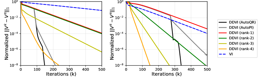
DDVI with AutoPI, AutoQR, different fixed ranks.

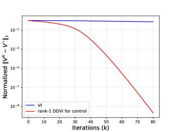
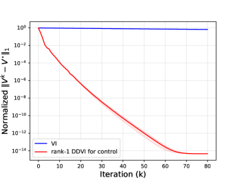
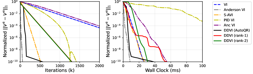
In Figure 1, we compare rank- $s$ DDVI for multiple values of $s$ and DDVI with AutoPI and AutoQR against the VI in Chain Walk and Maze. QR iteration (Section 2) is used to calculate $E_{s}$ with Schur vectors. In almost all cases, DDVI exhibits a significantly faster convergence rate compared to VI. Aligned with the theory, we observe that higher ranks achieve better convergence rates. Also, as DDVI with AutoPI and AutoQR progress and update $E_{s}$ , their convergence rate improves.

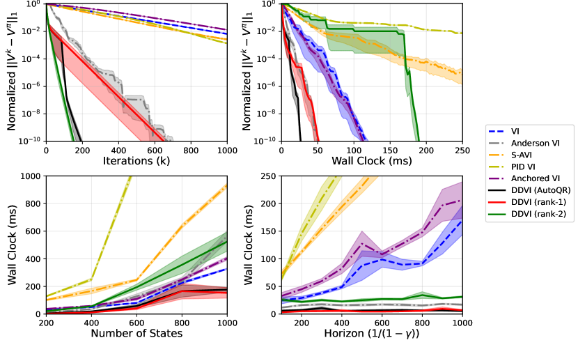
DDVI and other baselines.

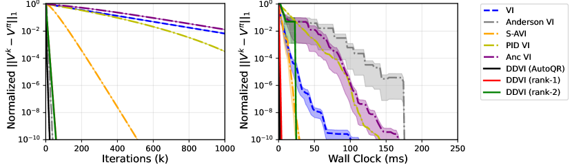
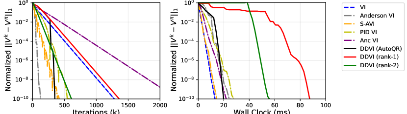
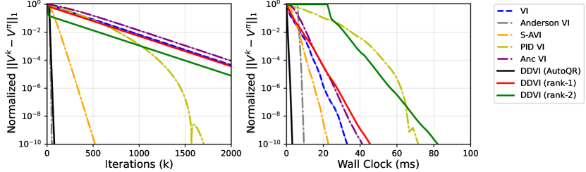
We perform an extensive comparison of DDVI against the prior accelerated VI methods: Safe Accelerated VI (S-AVI)[Goyal and Grand-Clément, 2022], Anderson VI [Geist and Scherrer, 2018], PID VI [Farahmand and Ghavamzadeh, 2021], and Anchored VI [Lee and Ryu, 2023]. In this experiment, we use the Implicitly Restarted Arnoldi Method [Lehoucq et al., 1998] from SciPy package to calculate the eigenvalues and eigenvectors for DDVI. Figure 2 (top-left) shows the convergence behaviour of the algorithms by iteration count in 20 randomly generated Garnet environments, where our algorithms outperform all the baselines. This comparison might not be fair as the amount of computation needed for each iteration of algorithms is not the same. Therefore, in Figure 2 (top-right), we compare the algorithms by wall clock time. It can be seen that rank- $2$ DDVI initially has to spend time to calculate $E_{s}$ before it starts to update the value function, but after the slow start, it has the fastest rate. The fast rate can compensate for the initial time if a high accuracy is needed. DDVI with AutoQR and rank- $1$ DDVI show a fast convergence from the beginning.

We further investigate how the algorithms scale with the size of MDP and the discount factor. Figure 2 (bottom-left) shows the runtime to reach a normalized error of $10^{-4}$ against the number of states. DDVI with AutoQR and rank- $1$ DDVI show the best scaling. Note that even rank- $2$ calculates a non-trivial $E_{s}$ also scales competitively. Figure 2 (bottom-right) show the scaling behaviour with horizon of the MDP, which is $1/(1-\gamma)$ . We measure the runtime to reach a normalized error of $10^{-4}$ for the horizon ranging from $100$ to $1000$ which corresponds to $\gamma$ ranging from $0.99$ to $0.999$ . Remarkably, DDVI algorithms have a low constant runtime even with long horizon tasks with $\gamma\approx 1$ . This is aligned with our theoretical result, as the rate $\gamma|\lambda_{s+1}|$ remains small as $\gamma$ approaches $1$ .

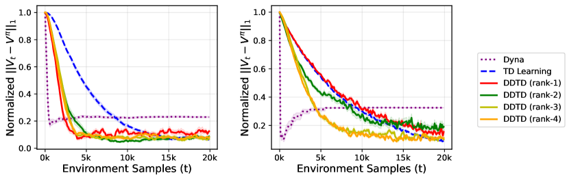
Rank- $s$ DDTD with QR iteration.

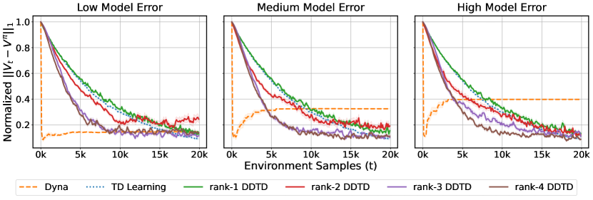
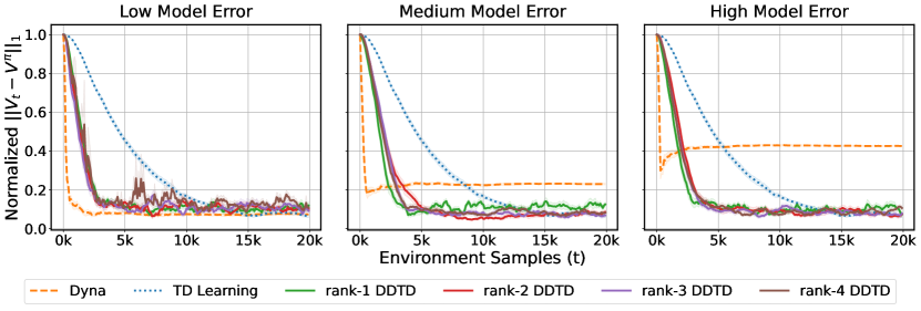
We compare DDTD with TD Learning and Dyna. For the sake of making the setting more realistic, we consider the case where the approximate model $\hat{\mathcal{P}}$ cannot exactly learn the true dynamics. Figure 3 shows that DDTD with large enough rank, can outperform TD. Note that unlike Dyna, DDTD does not suffer from model error, which shows that DDTD only uses the model for acceleration and is not a pure model-based algorithm.

7. Conclusion

In this work, we propose a framework for accelerating VI through matrix deflation. We theoretically analyzed our proposed methods DDVI and DDTD, and presented experimental results showing speedups in various setups.

The positive experimental results demonstrate matrix deflation to be a promising technique that may be applicable to a broader range of RL algorithms. One direction of future work is to extend the theoretical analysis DDVI for Control using a general rank- $s$ deflation matrix. Theoretically analyzing other RL methods combined with matrix deflation is another interesting direction.

Acknowledgements

AMF acknowledges the funding from the Natural Sciences and Engineering Research Council of Canada (NSERC) through the Discovery Grant program (2021-03701) and the Canada CIFAR AI Chairs program.

References

Akian et al. [2022] M. Akian, S. Gaubert, Z. Qu, and O. Saadi. Multiply accelerated value iteration for non-symmetric affine fixed point problems and application to Markov decision processes. SIAM Journal on Matrix Analysis and Applications, 43(1):199–232, 2022.
Andre et al. [1997] D. Andre, N. Friedman, and R. Parr. Generalized prioritized sweeping. Neural Information Processing Systems, 1997.
Azar et al. [2011] M. Azar, R. Munos, M. Ghavamzadeh, and H. Kappen. Speedy Q-learning. Neural Information Processing Systems, 2011.
Bacon [2018] P. Bacon. Temporal Representation Learning. PhD thesis, McGill University, 2018.
Bacon and Precup [2016] P. Bacon and D. Precup. A matrix splitting perspective on planning with options. arXiv:1612.00916, 2016.
Banach [1922] S. Banach. Sur les opérations dans les ensembles abstraits et leur application aux équations intégrales. Fundamenta Mathematicae, 3(1):133–181, 1922.
Bertsekas [1995] D. P. Bertsekas. Generic rank-one corrections for value iteration in markovian decision problems. Operations research letters, 17(3):111–119, 1995.
Bertsekas and Tsitsiklis [1996] D. P. Bertsekas and J. N. Tsitsiklis. Neuro-Dynamic Programming. Athena Scientific, 1996.
Bhandari et al. [2018] J. Bhandari, D. Russo, and R. Singal. A finite time analysis of temporal difference learning with linear function approximation. 2018.
Bhatnagar et al. [2009] S. Bhatnagar, R. S. Sutton, M. Ghavamzadeh, and M. Lee. Natural actor–critic algorithms. Automatica, 45(11):2471–2482, 2009.
Borkar [1998] Vivek S Borkar. Asynchronous stochastic approximations. SIAM Journal on Control and Optimization, 36(3):840–851, 1998.
Borkar and Meyn [2000] Vivek S Borkar and Sean P Meyn. The ode method for convergence of stochastic approximation and reinforcement learning. SIAM Journal on Control and Optimization, 38(2):447–469, 2000.
Bowen et al. [2021] W. Bowen, X. Huaqing, Z. Lin, L. Yingbin, and Z. Wei. Finite-time theory for momentum Q-learning. Conference on Uncertainty in Artificial Intelligence, 2021.
Bru et al. [2012] R. Bru, R. Canto, R. L. Soto, and A. M. Urbano. A Brauer’s theorem and related results. Central European Journal of Mathematics, 10:312–321, 2012.
Chen and Jiang [2019] J. Chen and N. Jiang. International conference on machine learning. Information-Theoretic Considerations in Batch Reinforcement Learning, 2019.
Chen et al. [2020] S. Chen, A. Devraj, A. Busic, and S. Meyn. Explicit mean-square error bounds for monte-carlo and linear stochastic approximation. International Conference on Artificial Intelligence and Statistics, 2020.
Chen et al. [2023] Z. Chen, S. T Maguluri, S. Shakkottai, and K. Shanmugam. A lyapunov theory for finite-sample guarantees of markovian stochastic approximation. Operations Research, 2023.
Dai et al. [2011] P. Dai, D. S. Weld, J. Goldsmith, et al. Topological value iteration algorithms. Journal of Artificial Intelligence Research, 42:181–209, 2011.
Dalal et al. [2018] G. Dalal, B. Szörényi, G. Thoppe, and S. Mannor. Finite sample analyses for td (0) with function approximation. Association for the Advancement of Artificial Intelligence, 2018.
Devraj and Meyn [2021] A. M. Devraj and S. P. Meyn. Q-learning with uniformly bounded variance. IEEE Transactions on Automatic Control, 67(11):5948–5963, 2021.
Ermis and Yang [2020] M. Ermis and I. Yang. A3DQN: Adaptive Anderson acceleration for deep Q-networks. IEEE Symposium Series on Computational Intelligence, 2020.
Ermis et al. [2021] M. Ermis, M. Park, and I. Yang. On Anderson acceleration for partially observable Markov decision processes. IEEE Conference on Decision and Control, 2021.
Ernst et al. [2005] D. Ernst, P. Geurts, and L. Wehenkel. Tree-based batch mode reinforcement learning. Journal of Machine Learning Research, 2005.
Even-Dar and Mansour [2003] E. Even-Dar and Y. Mansour. Learning rates for Q-learning. Journal of Machine Learning Research, 2003.
Fan et al. [2020] J. Fan, Z. Wang, Y. Xie, and Z. Yang. A theoretical analysis of deep Q-learning. Learning for dynamics and control, 2020.
Farahmand and Ghavamzadeh [2021] A. Farahmand and M. Ghavamzadeh. PID accelerated value iteration algorithm. International Conference on Machine Learning, 2021.
Farahmand et al. [2010] A. Farahmand, R. Munos, and C. Szepesvári. Error propagation for approximate policy and value iteration. Neural Information Processing Systems, 2010.
Geist and Scherrer [2018] M. Geist and B. Scherrer. Anderson acceleration for reinforcement learning. European Workshop on Reinforcement Learning, 2018.
Golub and Van Loan [2013] G. H. Golub and C. F. Van Loan. Matrix Computations. The John Hopkins University Press, 4th edition, 2013.
Gordon [1995] G. Gordon. Stable function approximation in dynamic programming. International Conference on Machine Learning, 1995.
Goyal and Grand-Clément [2022] V. Goyal and J. Grand-Clément. A first-order approach to accelerated value iteration. Operations Research, 71(2):517–535, 2022.
Grand-Clément [2021] J. Grand-Clément. From convex optimization to MDPs: A review of first-order, second-order and quasi-newton methods for MDPs. arXiv:2104.10677, 2021.
Gupta et al. [2015] A. Gupta, R. Jain, and P. W Glynn. An empirical algorithm for relative value iteration for average-cost MDPs. IEEE Conference on Decision and Control, 2015.
Hastings [1968] N. A. J. Hastings. Some notes on dynamic programming and replacement. Journal of the Operational Research Society, 19:453–464, 1968.
Hillen [2023] T. Hillen. Elements of Applied Functional Analysis. AMS Open Notes, 2023.
Hunter and Nachtergaele [2001] J. K. Hunter and B. Nachtergaele. Applied analysis. World Scientific Publishing Company, 2001.
Jaakkola et al. [1993] T. Jaakkola, M. Jordan, and S. Singh. Convergence of stochastic iterative dynamic programming algorithms. Advances in neural information processing systems, 1993.
Kushner and Kleinman [1968] H. Kushner and A. Kleinman. Numerical methods for the solution of the degenerate nonlinear elliptic equations arising in optimal stochastic control theory. IEEE Transactions on Automatic Control, 1968.
Kushner and Kleinman [1971] H. Kushner and A. Kleinman. Accelerated procedures for the solution of discrete Markov control problems. IEEE Transactions on Automatic Control, 1971.
Lagoudakis and Parr [2003] M. G. Lagoudakis and R. Parr. Least-squares policy iteration. Journal of Machine Learning Research, 2003.
Lakshminarayanan and Szepesvari [2018] C. Lakshminarayanan and C. Szepesvari. Linear stochastic approximation: How far does constant step-size and iterate averaging go? International Conference on Artificial Intelligence and Statistics, 2018.
Lee and Ryu [2023] J. Lee and E. K. Ryu. Accelerating value iteration with anchoring. Neural Information Processing Systems, 2023.
Lehoucq et al. [1998] R.B. Lehoucq, D.C. Sorensen, and C. Yang. ARPACK Users’ Guide: Solution of Large-scale Eigenvalue Problems with Implicitly Restarted Arnoldi Methods. Society for Industrial and Applied Mathematics, 1998.
Mackey [2008] L. Mackey. Deflation methods for sparse PCA. In Neural Information Processing Systems, 2008.
McMahan and Gordon [2005] H. B. McMahan and G. J. Gordon. Fast exact planning in Markov decision processes. International Conference on Automated Planning and Scheduling, 2005.
Meirovitch [1980] L. Meirovitch. Computational methods in structural dynamics. Springer Science & Business Media, 1980.
Meyn [2022] S. Meyn. Control Systems and Reinforcement Learning. Cambridge University Press, 2022.
Mnih et al. [2015] V. Mnih, K. Kavukcuoglu, D. Silver, A. A. Rusu, and et al. Human-level control through deep reinforcement learning. Nature, 518(7540):529–533, 2015.
Moore and Atkeson [1993] A. W. Moore and C. G. Atkeson. Prioritized sweeping: Reinforcement learning with less data and less time. Machine Learning, 1993.
Morgan [1995] R. B. Morgan. A restarted gmres method augmented with eigenvectors. SIAM Journal on Matrix Analysis and Applications, 16(4):1154–1171, 1995.
Munos and Szepesvári [2008] R. Munos and C. Szepesvári. Finite-time bounds for fitted value iteration. Journal of Machine Learning Research, 2008.
Park et al. [2022] M. Park, J. Shin, and I. Yang. Anderson acceleration for partially observable Markov decision processes: A maximum entropy approach. arXiv:2211.14998, 2022.
Peng and Williams [1993] J. Peng and R. J. Williams. Efficient learning and planning within the Dyna framework. Adaptive Behavior, 1(4):437–454, 1993.
Porteus [1975] E. L. Porteus. Bounds and transformations for discounted finite markov decision chains. Operations Research, 23(4):761–784, 1975.
Rakhsha et al. [2022] A. Rakhsha, A. Wang, M. Ghavamzadeh, and A. Farahmand. Operator splitting value iteration. Neural Information Processing Systems, 2022.
Reetz [1973] D. Reetz. Solution of a markovian decision problem by successive overrelaxation. Zeitschrift für Operations Research, 17:29–32, 1973.
Saad [2011] Y. Saad. Numerical methods for large eigenvalue problems: revised edition. SIAM, 2011.
Saad et al. [2000] Y. Saad, M. Yeung, J. Erhel, and F. Guyomarc’h. A deflated version of the conjugate gradient algorithm. SIAM Journal on Scientific Computing, 21(5):1909–1926, 2000.
Sharma et al. [2020] H. Sharma, M. Jafarnia-Jahromi, and R. Jain. Approximate relative value learning for average-reward continuous state mdps. Uncertainty in Artificial Intelligence, 2020.
Shi et al. [2019] W. Shi, S. Song, H. Wu, Y. Hsu, C. Wu, and G. Huang. Regularized Anderson acceleration for off-policy deep reinforcement learning. Neural Information Processing Systems, 2019.
Shroff and Keller [1993] G. M. Shroff and H. B. Keller. Stabilization of unstable procedures: the recursive projection method. SIAM Journal on numerical analysis, 30(4):1099–1120, 1993.
Sidford et al. [2023] A. Sidford, M. Wang, X. Wu, and Y. Ye. Variance reduced value iteration and faster algorithms for solving markov decision processes. Naval Research Logistics, 70(5):423–442, 2023.
Soto and Rojo [2006] R. L. Soto and O. Rojo. Applications of a Brauer theorem in the nonnegative inverse eigenvalue problem. Linear algebra and its applications, 416(2-3):844–856, 2006.
Sun et al. [2021] K. Sun, Y. Wang, Y. Liu, B. Pan, S. Jui, B. Jiang, L. Kong, et al. Damped Anderson mixing for deep reinforcement learning: Acceleration, convergence, and stabilization. Neural Information Processing Systems, 2021.
Sutton [1988] R. S. Sutton. Learning to predict by the methods of temporal differences. Machine Learning, 1988.
Sutton and Barto [2018] R. S. Sutton and A. G. Barto. Reinforcement Learning: An Introduction. The MIT Press, second edition, 2018.
Szepesvári [1997] C. Szepesvári. The asymptotic convergence-rate of Q-learning. Neural Information Processing Systems, 1997.
Szepesvári [2010] C. Szepesvári. Algorithms for Reinforcement Learning. Morgan Claypool Publishers, 2010.
Tsitsiklis and V. Roy [1997] J. N. Tsitsiklis and B. V. Roy. An analysis of temporal difference learning with function approximation. IEEE Transactions on Automatic Control, 1997.
Vieillard et al. [2020] N. Vieillard, B. Scherrer, O. Pietquin, and M. Geist. Momentum in reinforcement learning. International Conference on Artificial Intelligence and Statistics, 2020.
Wainwright [2019] M. J. Wainwright. Stochastic approximation with cone-contractive operators: Sharp $\ell_{\infty}$ -bounds for $q$ -learning. arXiv:1905.06265, 2019.
Watkins [1989] C. J. C. H. Watkins. Learning from Delayed Rewards. PhD thesis, King’s College, University of Cambride, 1989.
White [1963] D. J. White. Dynamic programming, markov chains, and the method of successive approximations. J. Math. Anal. Appl, 6(3):373–376, 1963.
Wingate et al. [2005] D. Wingate, K. D. Seppi, and S. Mahadevan. Prioritization methods for accelerating MDP solvers. Journal of Machine Learning Research, 2005.

Appendix

7.1. Prior works

Acceleration in RL.

Prioritized sweeping and its several variants [Moore and Atkeson, 1993, Peng and Williams, 1993, McMahan and Gordon, 2005, Wingate et al., 2005, Andre et al., 1997, Dai et al., 2011] specify the order of asynchronous value function updates, which may lead to accelerated convergence to the true value function. Speedy Q-learning [Azar et al., 2011] changes the update rule of Q-learning and employs aggressive learning rates to accelerate convergence. Sidford et al. [2023] accelerate the computation of $\mathcal{P}^{\pi}V^{k}$ by sampling it with variance reduction techniques. Recently, there has been a growing body of research that explores the application of acceleration techniques of other areas of applied math to planning and RL: Geist and Scherrer [2018], Sun et al. [2021], Ermis and Yang [2020], Park et al. [2022], Ermis et al. [2021], Shi et al. [2019] applies Anderson acceleration of fixed-point iterations, Lee and Ryu [2023] applies Anchor acceleration of minimax optimization, Vieillard et al. [2020], Goyal and Grand-Clément [2022], Grand-Clément [2021], Bowen et al. [2021], Akian et al. [2022] applies Nesterov acceleration of convex optimization, and Farahmand and Ghavamzadeh [2021] applies ideas inspired by PID controllers in control theory.

Matrix deflation.

Deflation techniques were first developed for eigenvalue computation [Meirovitch, 1980, Saad, 2011, Golub and Van Loan, 2013]. Matrix deflation, eliminating top eigenvalues of a given matrix with leaving the rest of the eigenvalues untouched, has been applied to various algorithms such as conjugate gradient algorithm [Saad et al., 2000], principal component analysis [Mackey, 2008], generalized minimal residual method [Morgan, 1995], and nonlinear fixed point iteration [Shroff and Keller, 1993] for improvement of convergence.

Some prior work in RL has explored subtracting constants from the iterates of VI, resulting in methods that resemble our rank- $1$ DDVI. For discounted MDP, Devraj and Meyn [2021] propose relative Q-learning, which can roughly be seen as the Q-learning version of rank-1 DDVI for Control, and Bertsekas [1995] proposes an extrapolation method for VI, which can be seen as rank-1 DDVI with shur deflation matrix for PE. White [1963] introduced relative value iteration in the context of undiscounted MDP with average reward, and several variants were proposed [Gupta et al., 2015, Sharma et al., 2020].

Matrix splitting of value iteration.

Matrix splitting has been studied in the RL literature to obtain an acceleration. Hastings [1968] and Kushner and Kleinman [1968] first suggested Gausss-Seidel iteration for computing value function. Kushner and Kleinman [1971] and Reetz [1973] applied Successive Over-Relaxation to VI and generalized Jacobi and Gauss-Seidel iteration. Porteus [1975] proposed several transformations of MDP that can be seen as a Gauss–Seidel variant of VI. Rakhsha et al. [2022] used matrix splitting with the approximate dynamics of the environment and extended to nonlinear operator splitting. Bacon and Precup [2016], Bacon [2018] analyzed planning with options through the matrix splitting perspective.

Convergence analysis of TD learning

Jaakkola et al. [1993] first proved the convergence of TD learning using the stochastic approximation (SA) technique. Borkar and Meyn [2000], Borkar [1998] suggested ODE-based framework to provide asymptotic convergence of SA including TD learning with an asynchronous update. Lakshminarayanan and Szepesvari [2018] study linear SA under i.i.d noise with respect to mean square error and Chen et al. [2020] study asymptotic convergence rate of linear SA under Markovian noise. Finite time analysis of TD learning first provided by Dalal et al. [2018] and extended to Markovian noise setting by Bhandari et al. [2018]. Leveraging Lyapunov theory, Chen et al. [2023] establishes finite time analysis of Markovian SA with an explicit bound.

8. Proof of Theoretical Results

8.1. Proof of Theorem 3.1

By definition of DDVI (2) and fixed point $V^{\pi}$ , we have

	$\displaystyle V^{k}-V^{\pi}$
	$\displaystyle=(I-\alpha\gamma E_{s})^{-1}((1-\alpha)I+\alpha\gamma(\mathcal{P}^{\pi}-E_{s}))(V^{k-1}-V^{\pi})$
	$\displaystyle=(I-\alpha\gamma E_{s})^{-1}((1-\alpha)(I-\alpha\gamma E_{s})^{-1}+\alpha\gamma(\mathcal{P}^{\pi}-E_{s})(I-\alpha\gamma E_{s})^{-1})((1-\alpha)I+\alpha\gamma(\mathcal{P}^{\pi}-E_{s}))(V^{k-2}-V^{\pi})$
	$\displaystyle=(I-\alpha\gamma E_{s})^{-1}((1-\alpha)(I-\alpha\gamma E_{s})^{-1}+\alpha\gamma(\mathcal{P}^{\pi}-E_{s})(I-\alpha\gamma E_{s})^{-1})^{k-1}((1-\alpha)I+\alpha\gamma(\mathcal{P}^{\pi}-E_{s}))(V^{0}-V^{\pi}),$

where $E_{s}$ is a rank- $s$ deflation matrix of $\mathcal{P}^{\pi}$ satisfying the conditions of Facts 1, 2, or 3. This implies that

\|V^{k}-V^{\pi}\|\leq C\left\|((1-\alpha)(I-\alpha\gamma E)^{-1}+\alpha\gamma(\mathcal{P}^{\pi}-E)(I-\alpha\gamma E)^{-1})^{k-1}\right\|\|V^{0}-V^{\pi}\|

for some constant $C\in$ .

First, suppose $E_{s}$ satisfies Facts 1 or 2. Let $U_{s}=[u_{1},\dots,u_{s}]$ and $V_{s}=[v_{1},\dots,v_{s}]$ . Define $D_{s,f(\lambda_{i})}=\text{diag}(f(\lambda_{1}),\dots,f(\lambda_{s}))$ for some function $f$ . Then $U_{s},V_{s},D_{s,f(\lambda_{i})}$ are $n\times s$ matrices and $E_{s}=U_{s}D_{s,\lambda_{i}}V_{s}^{\top}$ . By Jordan decomposition, $\mathcal{P}^{\pi}=UJU^{-1}$ where $J$ is Jordan matrix with $J_{ii}=\lambda_{i}$ for $i=1,\dots,n$ . Let $J_{s}$ be $s\times s$ submatrix of $J$ satisfying $(J_{s})_{ij}=J_{ij}$ for $1\leq i,j\leq s$ . Then, by condition of Theorem 3.1, $J_{s}=\text{diag}(\lambda_{1},\dots,\lambda_{s})=D_{s,\lambda_{i}}$ and $i$ -th column of $U$ is $u_{i}$ for $1\leq i\leq s$ . By simple calculation, we get $\mathcal{P}^{\pi}U_{s}=U_{s}J_{s}=U_{s}D_{s,\lambda_{i}}$ and $(I-\alpha\gamma E_{s})^{-1}=I+U_{s}D_{s,\frac{\gamma\alpha\lambda_{i}}{1-\gamma\alpha\lambda_{i}}}V^{\top}_{s}$ .

Since

	$\displaystyle(\mathcal{P}^{\pi}-U_{s}D_{s,\lambda_{i}}V^{\top}_{s})(U_{s}D_{s,\frac{\gamma\alpha\lambda_{i}}{1-\gamma\alpha\lambda_{i}}}V^{\top}_{s})$	$\displaystyle=U_{s}D_{s,\lambda_{i}}D_{s,\frac{\gamma\alpha\lambda_{i}}{1-\gamma\alpha\lambda_{i}}}V^{\top}_{s}-U_{s}D_{s,\lambda_{i}}D_{s,\frac{\gamma\alpha\lambda_{i}}{1-\gamma\alpha\lambda_{i}}}V^{\top}_{s}$
		$\displaystyle=0,$

we get

\displaystyle(\mathcal{P}^{\pi}-E_{s})(I-\alpha\gamma E_{s})^{-1}

\displaystyle=\mathcal{P}^{\pi}-E_{s}.

Then,

	$\displaystyle(1-\alpha)(I-\alpha\gamma E_{s})^{-1}+\alpha\gamma(\mathcal{P}^{\pi}-E_{s})(I-\alpha\gamma E_{s})^{-1}$
	$\displaystyle=(1-\alpha)\left(I+U_{s}D_{s,\frac{\gamma\alpha\lambda_{i}}{1-\gamma\alpha\lambda_{i}}}V^{\top}_{s}\right)+\alpha\gamma\left(UJU^{-1}-U_{s}D_{s,\lambda_{i}}V^{\top}_{s}\right)$
	$\displaystyle=(1-\alpha)I+\alpha\gamma UJU^{-1}+U_{s}D_{s,\frac{(\lambda_{i}\gamma-1)\gamma\alpha^{2}\lambda_{i}}{1-\gamma\alpha\lambda_{i}}}V^{\top}_{s}$
	$\displaystyle=U\left((1-\alpha)I+\alpha\gamma J+e_{1:s}D_{s,\frac{(\lambda_{i}\gamma-1)\gamma\alpha^{2}\lambda_{i}}{1-\gamma\alpha\lambda_{i}}}V_{s}^{\top}U\right)U^{-1},$

where $e_{i}\in\mathbb{R}^{n}$ is $i$ -th unit vector and $e_{1:s}=[e_{1},\dots,e_{s}]$ , and $(1-\alpha)I+\alpha\gamma J+e_{1:s}D_{s,\frac{(\lambda_{i}\gamma-1)\gamma\alpha^{2}\lambda_{i}}{1-\gamma\alpha\lambda_{i}}}V_{s}^{\top}U$ is upper traingular matrix with diagonal entries $\frac{(1-\alpha)}{1-\alpha\gamma\lambda_{1}},\dots,\frac{(1-\alpha)}{1-\alpha\gamma\lambda_{s}},(1-\alpha)+\alpha\gamma\lambda_{s+1},\dots,(1-\alpha)+\alpha\gamma\lambda_{n}$ .

Now suppose $E_{s}=\sum_{i=1}^{s}\lambda_{i}u_{i}u_{i}^{\top}$ satisfies Fact 3. Similarly, let $U_{s}=[u_{1},\dots,u_{s}]$ . Then, $E_{s}=U_{s}D_{s,\lambda_{i}}U^{\top}_{s}$ . By Schur decomposition, $\mathcal{P}^{\pi}=URU^{\top}$ where $R$ is an upper triangular matrix with $R_{ii}=\lambda_{i}$ for $i=1,\dots,n$ , and $U$ is a unitary matrix. By simple calculation, we have $\mathcal{P}^{\pi}U_{s}=U_{s}R_{s}$ where $R_{s}$ is $s\times s$ submatrix of $R$ such that $(R_{s})_{ij}=R_{ij}$ for $1\leq i,j\leq s$ and $(I-\alpha\gamma E_{s})^{-1}=I+U_{s}D_{s,\frac{\gamma\alpha\lambda_{i}}{1-\gamma\alpha\lambda_{i}}}U^{\top}_{s}$ .

Since

	$\displaystyle(\mathcal{P}^{\pi}-U_{s}D_{s,\lambda_{i}}U^{\top}_{s})(U_{s}D_{s,\frac{\gamma\alpha\lambda_{i}}{1-\gamma\alpha\lambda_{i}}}U^{\top}_{s})$	$\displaystyle=U_{s}R_{s}D_{s,\frac{\gamma\alpha\lambda_{i}}{1-\gamma\alpha\lambda_{i}}}U^{\top}_{s}-U_{s}D_{s,\lambda_{i}}D_{s,\frac{\gamma\alpha\lambda_{i}}{1-\gamma\alpha\lambda_{i}}}U^{\top}_{s}$
		$\displaystyle=U_{s}(R_{s}-D_{s,\lambda_{i}})D_{s,\frac{\gamma\alpha\lambda_{i}}{1-\gamma\alpha\lambda_{i}}}U^{\top}_{s},$

we get

	$\displaystyle(\mathcal{P}^{\pi}-E_{s})(I-\alpha\gamma E_{s})^{-1}$	$\displaystyle=(\mathcal{P}^{\pi}-U_{s}D_{s,\lambda_{i}}U^{\top}_{s})(I+U_{s}D_{s,\frac{\gamma\alpha\lambda_{i}}{1-\gamma\alpha\lambda_{i}}}U^{\top}_{s})$
		$\displaystyle=(\mathcal{P}^{\pi}-U_{s}D_{s,\lambda_{i}}U^{\top}_{s})+U_{s}(R_{s}-D_{s,\lambda_{i}})D_{s,\frac{\gamma\alpha\lambda_{i}}{1-\gamma\alpha\lambda_{i}}}U^{\top}_{s}.$

Then,

	$\displaystyle(1-\alpha)(I-\alpha\gamma E_{s})^{-1}+\alpha\gamma(\mathcal{P}^{\pi}-E_{s})(I-\alpha\gamma E_{s})^{-1}$
	$\displaystyle=(1-\alpha)I+(1-\alpha)U_{s}D_{s,\frac{\gamma\alpha\lambda_{i}}{1-\gamma\alpha\lambda_{i}}}U^{\top}_{s}+\alpha\gamma URU^{\top}-\alpha\gamma U_{s}D_{s,\lambda_{i}}U^{\top}_{s}+\alpha\gamma U_{s}(R_{s}-D_{s,\lambda_{i}})D_{s,\frac{\gamma\alpha\lambda_{i}}{1-\gamma\alpha\lambda_{i}}}U^{\top}_{s}$
	$\displaystyle=(1-\alpha)I+\alpha\gamma URU^{\top}+U_{s}\left(D_{s,\frac{(1-\alpha)\gamma\alpha\lambda_{i}}{1-\gamma\alpha\lambda_{i}}}-D_{s,\alpha\gamma\lambda_{i}}+\alpha\gamma(R_{s}-D_{s,\lambda_{i}})D_{s,\frac{\gamma\alpha\lambda_{i}}{1-\gamma\alpha\lambda_{i}}}\right)U^{\top}_{s}$
	$\displaystyle=(1-\alpha)I+\alpha\gamma URU^{\top}+U_{s}\left(D_{\frac{(\lambda_{i}\gamma-1)\gamma\alpha^{2}\lambda_{i}}{1-\gamma\alpha\lambda_{i}}}+\alpha\gamma(R_{s}-D_{\lambda_{i}})D_{\frac{\gamma\alpha\lambda_{i}}{1-\gamma\alpha\lambda_{i}}}\right)U^{\top}_{s}$
	$\displaystyle=(1-\alpha)I+\alpha\gamma URU^{\top}+U_{s}R_{s,\frac{(\lambda_{i}\gamma-1)\gamma\alpha^{2}\lambda_{i}}{1-\gamma\alpha\lambda_{i}}}U^{\top}_{s}$
	$\displaystyle=U\left((1-\alpha)I+\alpha\gamma R+e_{1:s}R_{s,\frac{(\lambda_{i}\gamma-1)\gamma\alpha^{2}\lambda_{i}}{1-\gamma\alpha\lambda_{i}}}e_{1:s}^{\top}\right)U^{\top}$

where $R_{s,\frac{(\lambda_{i}\gamma-1)\gamma\alpha^{2}\lambda_{i}}{1-\gamma\alpha\lambda_{i}}}$ is $s\times s$ upper triangular matrix with digonal entries $\frac{(\lambda_{1}\gamma-1)\gamma\alpha^{2}\lambda_{1}}{1-\gamma\alpha\lambda_{1}},\dots,\frac{(\lambda_{s}\gamma-1)\gamma\alpha^{2}\lambda_{s}}{1-\gamma\alpha\lambda_{s}}$ , satisfying $R_{s,\frac{(\lambda_{i}\gamma-1)\gamma\alpha^{2}\lambda_{i}}{1-\gamma\alpha\lambda_{i}}}=D_{s,\frac{(\lambda_{i}\gamma-1)\gamma\alpha^{2}\lambda_{i}}{1-\gamma\alpha\lambda_{i}}}+\alpha\gamma(R_{s}-D_{s,\lambda_{i}})D_{s,\frac{\gamma\alpha\lambda_{i}}{1-\gamma\alpha\lambda_{i}}}$ . By simple calculation, we know that $(1-\alpha)I+\alpha\gamma R+e_{1:s}R_{\frac{(\alpha\lambda_{i}\gamma-\alpha)\gamma\alpha\lambda_{i}}{1-\gamma\alpha\lambda_{i}}}e_{1:s}^{\top}$ is $n\times n$ upper triangular matrix with digonal entries $\frac{(1-\alpha)}{1-\alpha\gamma\lambda_{1}},\dots,\frac{(1-\alpha)}{1-\alpha\gamma\lambda_{s}},(1-\alpha)+\alpha\gamma\lambda_{s+1},\dots,(1-\alpha)+\alpha\gamma\lambda_{n}$ .

Therefore, by spectral analysis, we conclude that

\displaystyle\|V^{k}-V^{\pi}\|=\tilde{O}(|\lambda|^{k}\|V^{0}-V^{\pi}\|)

as $k\rightarrow\infty$ , where

\lambda=\max_{1\leq i\leq s,s+1\leq j\leq n}\Big{\{}\left|\frac{1-\alpha}{1-\alpha\gamma\lambda_{i}}\right|,\left|1-\alpha+\alpha\gamma\lambda_{j}\right|\Big{\}}.

8.2. Proof of Collorary 3.2

Putting $\alpha=1$ in Theorem 3.1, we conclude Corollary 3.2.

8.3. Proof of Theorem 4.1

By definition of DDVI for Control (3),

\displaystyle V^{k}-V^{\star}=\left(I+\frac{\gamma}{1-\gamma}E_{1}\right)\left(W^{k}-\left(I-\gamma E_{1}\right)V^{\star}\right)

where $E_{1}=\mathbf{1}v^{\top}$ . Let $W^{\star}=\left(I-\gamma E_{1}\right)V^{\star}$ . Note that

	$\displaystyle\max_{\pi}\{r^{\pi}+\gamma({\mathcal{P}}^{\pi}-E_{1})W^{\star}\}$	$\displaystyle=\max_{\pi}\{r^{\pi}+\gamma({\mathcal{P}}^{\pi}-E_{1})V^{\star}\}$
		$\displaystyle=\max_{\pi}\{r^{\pi}+\gamma{\mathcal{P}}^{\pi}V^{\star}\}-\gamma E_{1}V^{\star}$
		$\displaystyle=W^{\star}.$

Thus,

\displaystyle W^{k}-W^{\star}=\gamma\left({\mathcal{P}^{\pi_{g}}-E_{1}}\right)W^{k-1}+r^{\pi_{g}}-\gamma\left({\mathcal{P}^{\pi^{\star}}-E_{1}}\right)W^{\star}-r^{\pi^{\star}}

where $\pi_{g}=\operatorname*{argmax}_{\pi}\{r^{\pi}+\gamma({\mathcal{P}}^{\pi}-E_{1})W^{k-1}\}$ and $\pi^{\star}$ is optimal policy. This implies that

	$\displaystyle W^{k}-W^{\star}$	$\displaystyle\leq\gamma\left({\mathcal{P}^{\pi_{g}}-E_{1}}\right)(W^{k-1}-W^{\star}),$
	$\displaystyle W^{k}-W^{\star}$	$\displaystyle\geq\gamma\left({\mathcal{P}^{\pi^{\star}}-E_{1}}\right)(W^{k-1}-W^{\star}),$

and

\displaystyle\gamma\mathcal{P}^{\pi^{\star}}(W^{k-1}-W^{\star})\leq W^{k}-W^{\star}+\gamma E_{1}(W^{k-1}-W^{\star})

\displaystyle\leq\gamma\mathcal{P}^{\pi_{g}}(W^{k-1}-W^{\star}).

Then, there exist $0\leq t_{i}\leq 1$ such that

t_{i}\left({\gamma\mathcal{P}^{\pi^{\star}}(W^{k-1}-W^{\star})}\right)_{i}+(1-t_{i})\left({\gamma\mathcal{P}^{\pi_{g}}(W^{k-1}-W^{\star})}\right)_{i}=\left({W^{k}-W^{\star}+\gamma E_{1}(W^{k-1}-W^{\star})}\right)_{i}

for $1\leq i\leq n$ . Define $\pi_{k}(a\,|\,i)=t_{i}\pi^{\star}(a\,|\,i)+(1-t_{i})\pi_{g}(a\,|\,i)$ for all $a\in\mathcal{A}$ and $1\leq i\leq n$ . Then $\pi_{k}$ satisfies

\displaystyle W^{k}-W^{\star}=\gamma\left({\mathcal{P}^{\pi_{k}}-E_{1}}\right)(W^{k-1}-W^{\star}).

Thus, we get

	$\displaystyle W^{k}-W^{\star}$	$\displaystyle=\gamma^{k}\prod_{i=1}^{k}\left({\mathcal{P}^{\pi_{i}}-E_{1}}\right)(W^{0}-W^{\star})$
		$\displaystyle=\gamma^{k}\prod_{i=1}^{k}\left({\mathcal{P}^{\pi_{i}}-E_{1}}\right)(I-\gamma E_{1})(V^{0}-V^{\star})$
		$\displaystyle=\gamma^{k}\left({\mathcal{P}^{\pi_{k}}-E_{1}}\right)\prod_{i=1}^{k-1}\mathcal{P}^{\pi_{i}}(V^{0}-V^{\star}),$

and this implies that

	$\displaystyle V^{k}-V^{\star}$	$\displaystyle=\gamma^{k}\left(I+\frac{\gamma}{1-\gamma}E_{1}\right)\left({\mathcal{P}^{\pi_{k}}-E_{1}}\right)\prod_{i=1}^{k-1}\mathcal{P}^{\pi_{i}}(V^{0}-V^{\star})$
		$\displaystyle=\gamma^{k}\left(\mathcal{P}^{\pi_{k}}+\frac{\gamma}{1-\gamma}E_{1}\mathcal{P}^{\pi_{k}}-\frac{1}{1-\gamma}\mathbf{1}v^{\top}\right)\prod_{i=1}^{k-1}\mathcal{P}^{\pi_{i}}(V^{0}-V^{\star}).$

Then, we have

\|V^{k}-V^{\star}\|\leq\frac{2}{1-\gamma}\gamma^{k}\|V^{0}-V^{\star}\|

since $E_{1}\mathcal{P}^{\pi_{k}}$ is stochastic matrix with $\|E_{1}\mathcal{P}^{\pi_{k}}\|=1$ .

Suppose there exist unique optimal policy $\pi^{\star}$ . Then, if (non-deflated) VI generates $V^{k}$ for $k=0,1,\dots$ , there exist $K$ such that $\operatorname*{argmax}_{\pi}T^{\pi}V^{k}=\pi^{\star}$ for $k>K$ . Since DDVI for Control generates same policy with VI for Control, DDVI for Control also generates greedy policy $\pi^{\star}$ for $k>K$ iterations. Therefore, we get

	$\displaystyle\\|V^{k}-V^{\star}\\|$	$\displaystyle=\left\\|\gamma^{k}\left(I+\frac{\gamma}{1-\gamma}\mathbf{1}v^{\top}\right)\left(\mathcal{P}^{\pi^{\star}}-E_{1}\right)^{k-K}\prod_{i=1}^{K}\left({\mathcal{P}^{\pi_{i}}-E_{1}}\right)(V^{0}-V^{\star})\right\\|$
		$\displaystyle=C\gamma^{k}\left\\|\left(\mathcal{P}^{\pi^{\star}}-E_{1}\right)^{k-K}\right\\|\\|V^{0}-V^{\star}\\|$
		$\displaystyle=\tilde{O}(\|\gamma\lambda_{2}\|^{k}\\|V^{0}-V^{\star}\\|)$

for $k>K$ and some constant $C\in$ .

8.4. Proof of Theorem 5.1

Consider following stochastic approximation algorithm

\displaystyle Y^{k+1}=Y^{k}+\eta_{k}f(Y^{k},\zeta_{k})

(5)

for $k=0,1,\dots$ , where $Y^{k}\in^{n}$ , $\eta_{k}\in^{+}$ , $f(\cdot,z):^{n}\rightarrow^{n}$ is uniformly Lipschitz, and $\{\zeta_{k}\}_{k=0,1,\dots}$ are i.i.d random variables. Let $F(y)=\mathbf{E}[f(y,\zeta_{k})]$ , $F_{\infty}(y)=\lim_{r\rightarrow\infty}F(ry)/r$ , $M^{k+1}=f(Y^{k},\zeta_{k})-F(Y^{t})$ , and $\mathcal{F}^{k}=\sigma(Y^{i},M^{i},1\leq i\leq t)$ . Then following proposition holds.

Proposition 8.1.

[Borkar and Meyn, 2000, Theorem 2.2 and 2.5] If (i) $\eta_{k}=(k+1)^{-1}$ , (ii) $\{M^{k},\mathcal{F}^{k}\}_{k=0,1,\dots,}$ are martingale difference sequence , (iii) $\mathbf{E}[M^{k+1}\,|\,\mathcal{F}^{k}]\leq K(1+\|Y^{k}\|^{2})$ for some constant $K$ , (iv) $\dot{y}(t)=F_{\infty}(y(t))$ has asymptotically stable equilibrium origin, and (v) $\dot{y}(t)=F(y(t))$ has a unique globally asymtotically stable equilibrium $y^{\star}$ , then $\{Y^{t}\}_{k=0,1,\dots}$ of (5) converges to $y^{\star}$ almost surely, and furthermore, $\{Y^{t}\}_{k=0,1,\dots}$ of

\displaystyle Y^{k+1}(i_{k})=Y^{k}(i_{k})+\eta_{\nu_{i_{k},t}}f(Y^{k},\zeta_{k})(i_{k})

(6)

for $k=0,1,\dots$ where $i_{k}$ is random variable taking a value in $\{1,2,\cdots,n\}$ , $\nu_{i,t}=\sum^{k}_{k=0}\mathbf{1}_{\{i=i_{k}\}}$ satisfying $\liminf\nu_{i,t}/t>c$ for some constant $c>0$ , also converge to $y^{\star}$ almost surely.

In (6), $Y^{k}(i_{k})$ and $f(Y^{k},\zeta_{k})(i_{k})$ are $i$ -th coordinate of $Y^{k}$ and $f(Y^{k},\zeta_{k})$ , respectively. (6) can be interpreted as asynchronous version of (5), and we note that Proposition 8.1 is a simplified version with stronger conditions of Theorem 2.2 and 2.5 of Borkar and Meyn [2000].

Recall that DDTD (4) with $\alpha=1$ is

	$\displaystyle W^{k+1}(X_{k})$	$\displaystyle=W^{k}(X_{k})+\eta_{\nu_{i,t}}\big{[}r^{\pi}(X_{k})+\gamma V^{k}(X_{k}^{\prime})-\gamma(E_{s}V^{k})(X_{k})-W^{k}(X_{k})\big{]}$
	$\displaystyle V^{k+1}$	$\displaystyle=\left(I-\gamma E_{s}\right)^{-1}W^{k+1}.$		(7)

We will first show that $W^{k}\rightarrow(I-\gamma E_{s})V^{\pi}$ and this directly implies that $V^{k}\rightarrow V^{\pi}$ . For applying Proposition 8.1, consider

\displaystyle W^{k+1}=W^{k}+\eta_{k}f(W^{k},Z_{t})

where $\eta_{k}=(k+1)^{-1}$ , $Z_{t}\in^{n}$ such that $Z_{t}(x)\sim\mathcal{P}^{\pi}(\cdot\,|\,x)$ and $\{Z_{t}\}_{k=0,1,\dots}$ are i.i.d random variables, and $f(W^{k},Z_{t})(x)=r^{\pi}(x)+\gamma(\left(I-\gamma E_{s}\right)^{-1}W^{k})(Z_{t}(x))-\gamma E_{s}\left(I-\gamma E_{s}\right)^{-1}W^{k}(x)-W^{k}(x)$ . Then, $F(W)=\mathbf{E}[f(W,Z_{t})]=[\gamma(\mathcal{P}^{\pi}-E_{s})(I-\gamma E_{s})^{-1}-I]W+r^{\pi}$ , $M^{k+1}=f(W^{k},Z_{t})-F(W^{k})$ , and $\mathcal{F}^{k}=\sigma(W^{i},M^{i},1\leq i\leq t)$ .

We now check the conditions. First, since $f(W,z)(x)-f(W^{\prime},z)(x)=\left(I-\gamma E_{s}\right)^{-1}(W-W^{\prime})(z(x))-(I+\gamma E_{s}\left(I-\gamma E_{s}\right)^{-1})(W-W^{\prime})(x)$ implies $\|f(W,z)-f(W^{\prime},z)\|\leq(\|\left(I-\gamma E_{s}\right)^{-1}\|+\|(I+\gamma E_{s}\left(I-\gamma E_{s}\right)^{-1})\|)\|W-W^{\prime}\|$ , $f(\cdot,z)$ is uniformly Lipschitz.

	$\displaystyle\mathbf{E}[M^{k+1}(x)\,\|\,\mathcal{F}_{t}]$
	$\displaystyle=\mathbf{E}[\gamma(\left(I-\gamma E_{s}\right)^{-1}W^{k})(Z_{t}(x))-\gamma(E_{s}\left(I-\gamma E_{s}\right)^{-1}W^{k})(x)-\gamma((\mathcal{P}^{\pi}-E_{s}))(I-\gamma E_{s})^{-1}W^{k})(x)\,\|\,\mathcal{F}^{k}]$
	$\displaystyle=\gamma\mathcal{P}^{\pi}\left(I-\gamma E_{s}\right)^{-1}W^{k})(x)-\gamma\mathcal{P}^{\pi}(I-\gamma E_{s})^{-1}W^{k}(x)$
	$\displaystyle=0$

for all $x\in\mathcal{X}$ . This implies that $M^{k+1}$ is martingale difference sequence. Also, $\mathbf{E}[\|M^{k+1}\|^{2}\,|\,\mathcal{F}^{k}]\leq(\|\gamma\left(I-\gamma E_{s}\right)^{-1}\|+\|\gamma\mathcal{P}^{\pi}(I-\gamma E_{s})^{-1}\|)^{2}\|W^{k}\|^{2}\leq K(1+\|{W^{k}}\|^{2})$ for constant $K=(\|\gamma\left(I-\gamma E_{s}\right)^{-1}\|+\|\gamma\mathcal{P}^{\pi}(I-\gamma E_{s})^{-1}\|)^{2}$ .

By definition, $F_{\infty}(y)=\lim_{r\rightarrow\infty}F(ry)/r=\gamma(\mathcal{P}^{\pi}-E_{s}))(I-\gamma E_{s})^{-1}-I]y$ . In Section 8.1, we showed that $\text{spec}(F_{\infty}+I)=\{\gamma\lambda_{s+1},\dots,\gamma\lambda_{n},0\}$ . Hence, $\text{spec}(F_{\infty})=\{\gamma\lambda_{s+1}-1,\dots,\gamma\lambda_{1}-1,-1\}$ . Since $|\lambda_{i}|\leq 1$ for all $s+1\leq i\leq n$ , real parts of all eigenvalues $F_{\infty}$ are negative. This implies that $\dot{y}(t)=F_{\infty}(y(t))$ , has an asymtotically stable equilibrium origin and $\dot{y}(t)=F(y(t))$ has a unique globally asymtotically stable equilibrium $W^{\pi}=[I-(\gamma(\mathcal{P}^{\pi}-E_{s}))(I-\gamma E_{s})^{-1}]^{-1}r^{\pi}$ .

Lastly, since $X_{k}\sim\text{Unif}(\mathcal{X})$ and $\{X_{k}\}_{k=0,1,\dots}$ are i.i.d random variables, $\nu_{i,t}/t$ converges to $\frac{1}{n}$ almost suerly by law of large numbers. Since $\eta_{\nu_{X_{k},t}}=(\sum^{k}_{i=0}\mathbf{1}_{X_{k}=X_{i}})^{-1}$ , Therefore, by Proposition 8.1, $\{W^{k}\}_{k=0,1,\dots}$ of (7) converge to $W^{\pi}$ almost surely, and this implies that $V^{k}\rightarrow(I-\gamma E_{s})^{-1}W^{\pi}=(I-\gamma\mathcal{P}^{\pi})^{-1}r^{\pi}=V^{\pi}$ almost surely.

8.5. Proof of Theorem 5.2

Consider following linear stochastic approximation algorithm

\displaystyle Y^{k+1}=Y^{k}+\eta_{k}(A(\zeta_{k})Y^{t}+b(\zeta_{k}))

(8)

for $k=0,1,\dots$ , where $Y^{k}\in^{n}$ , $\{\zeta_{k}\}_{k=0,1,\dots,}$ are random variables, $b(\zeta_{k})\in^{n}$ , $A(\zeta_{k})\in^{n}\times^{n}$ , and $\|A_{i,j}\|,\|b_{k}\|<\infty$ , for $1\leq i,j\leq n$ and $1\leq k\leq n$ . Then, following Proposition holds.

Proposition 8.2.

[Chen et al., 2020, Theorem 2.5 and 2.7] If (i) $\eta_{k}=g(k+1)^{-1}$ for $g>0$ , (ii) $\{\zeta_{k}\}_{k=0,1,\dots}$ is ergodic (aperiodic and irreducible) Markov process with unique invariant measure $\mu$ , (iii) $\mathbf{E}_{\mu}[A^{t}]=A$ and $\mathbf{E}_{\mu}[B^{t}]=b$ , (iv) $A$ is Hurwitz, (v) $Re(\lambda)<-1/2$ for all $\lambda\in$ spec( $gA$ ), then $\mathbf{E}[\|Y^{t}-Y^{\star}\|^{2}]=O(k^{-1})$ where $Y^{\star}=-A^{-1}b$ .

We note that Proposition 8.1 is also a simplified version with stronger conditions of Theorem 2.5 and 2.7 of Chen et al. [2020].

Define $\psi(X_{k})\in^{n}$ as $\psi(X_{k})(x)=\mathbf{1}_{\{X_{k}=x\}}$ . Then, DDTD (4) with $\alpha=1$ is equivalent to

W^{k+1}=W^{k}+\eta_{k}(A(X_{k},X^{\prime}_{k})W^{k}+b(X_{k},X^{\prime}_{k})),

where $A(X,X^{\prime})=\psi(X)(\psi(X^{\prime})^{\top}\gamma\left(I-\gamma E_{s}\right)^{-1}-\psi(X)^{\top}\gamma E_{s}\left(I-\gamma E_{s}\right)^{-1}-\psi(X)^{\top})$ and $b(X,X^{\prime})=\psi(X)r^{\pi}(X)$ . Hence $\|A_{i,j}\|,\|b_{k}\|<\infty$ , for $1\leq i,j\leq n$ and $1\leq k\leq n$ .

Since $\{X_{k},X^{\prime}_{k}\}_{k=0,1,\dots}$ are i.i.d random variables, $\{X_{k},X^{\prime}_{k}\}_{k=0,1,\dots}$ are Markov process. Let $\mu\sim\{X_{k},X^{\prime}_{k}\}$ and $\mathcal{P}(x_{1},x^{\prime}_{1}\,|\,x_{2},x^{\prime}_{2})$ be transition matrix of $\{X_{k},X^{\prime}_{k}\}_{k=0,1,\dots}$ . Then $\mathcal{P}(x_{1},x^{\prime}_{1}\,|\,x_{2},x^{\prime}_{2})=\mu(x_{1},x_{1}^{\prime})=\frac{1}{n}\mathcal{P}^{\pi}(x^{\prime}_{1}\,|\,x_{1})$ . Since $(\mu^{\prime})^{\top}\mathcal{P}(\cdot,\cdot\,|\,\cdot,\cdot)=\mu$ for any distribution $\mu^{\prime}$ , $\mu$ is unique invarinat measure. Hence, $\{X_{k},X^{\prime}_{k}\}_{k=0,1,\dots}$ is irreducible and aperiodic.

	$\displaystyle\mathbf{E}_{\mu}[A(X_{k},X^{\prime}_{k})]$	$\displaystyle=\mathbf{E}_{\mu}[\psi(X_{k})(\psi(X^{\prime}_{k})^{\top}\gamma\left(I-\gamma E_{s}\right)^{-1}-\psi(X_{t})^{\top}\gamma E_{s}\left(I-\gamma E_{s}\right)^{-1}-\psi(X_{k})^{\top})\,\|\,X_{k}]$
		$\displaystyle=\mathbf{E}_{\mu}[\psi(X_{k})(\psi(X_{k})^{\top}\mathcal{P}^{\pi}\left(I-\gamma E_{s}\right)^{-1}-\psi(X_{t})^{\top}\gamma E_{s}\left(I-\gamma E_{s}\right)^{-1}-\psi(X_{k})^{\top})]$
		$\displaystyle=\mathbf{E}_{\mu}[\psi(X_{k})\psi(X_{k})^{\top}(\mathcal{P}^{\pi}\left(I-\gamma E_{s}\right)^{-1}-\gamma E_{s}\left(I-\gamma E_{s}\right)^{-1}-I)]$
		$\displaystyle=n^{-1}((\mathcal{P}^{\pi}-\gamma E_{s})\left(I-\gamma E_{s}\right)^{-1}-I)$

and $\mathbf{E}_{\mu}[b(X_{k},X^{\prime}_{k})]=n^{-1}r^{\pi}$ . Then, $Y^{\star}=-A^{-1}b=[I-(\gamma(\mathcal{P}^{\pi}-E_{s}))(I-\gamma E_{s})^{-1}]^{-1}r^{\pi}=W^{\pi}$ .

As we discussed in Section 8.4, $\text{spec}(A)=\{\gamma\lambda_{s+1}-1,\dots,\gamma\lambda_{n}-1,-1\}$ . Let $\lambda_{\text{DDTD}}=\min_{\lambda\in\{\lambda_{s+1},\dots,\lambda_{n}\}}\text{Re}(1-\gamma\lambda)$ . Then, if $g>\frac{n}{2\lambda_{\text{DDTD}}}$ , $Re(\lambda)<-1/2$ for all $\lambda\in$ spec( $gA$ ). Therefore, by Proposition 8.2, $\mathbf{E}[\|W^{k}-W^{\pi}\|^{2}]=O(k^{-1})$ and this implies that $\mathbf{E}[\|V^{k}-V^{\pi}\|^{2}]\leq\mathbf{E}[\|(I-\gamma E_{s})^{-1}\|^{2}\|W^{k}-W^{\star}\|^{2}]=O(k^{-1})$ .

8.6. Non-asymptotic convergence analysis of DDTD

Consider following the stochastic approximation algorithm

\displaystyle Y^{k+1}=Y^{k}+\eta_{k}(f(Y^{k},\zeta_{k})-Y^{k}+Z_{k})

(9)

for $k=0,1,\dots$ , where $Y^{k}\in^{n}$ , $\eta_{k}\in^{+}$ , $\{\zeta_{k}\}_{k=0,1,\dots}$ are Markov chain with unique distribution $\mu$ and transition matrix $P$ . Let $F(y)=\mathbf{E}[f(y,\zeta_{k})]$ and $\mathcal{F}^{k}=\sigma(Y^{i},M^{i},Z_{i},\eta_{i}1\leq i\leq t)$ . Define mixing time as $t_{\delta}=\{\min{k\geq 0,:\max_{y}\|P^{k}(\cdot,y)-\mu(\cdot)\|_{\text{TV}}}<\delta\}$ where $\|\cdot\|_{\text{TV}}$ stands for the total variation distance. Let $Y^{\star}$ be fixed point of $F(y)$ . Then following proposition holds.

Proposition 8.3.

[Chen et al., 2023, Theorem 1] Let (i) $\{\zeta_{k}\}_{k=0,1,\dots}$ is aperiodic and irreducible Markov chain, (ii) $F$ is $\beta$ -contraction respect to some $\|\cdot\|_{c}$ , (iii) $f(\cdot,z):^{n}\rightarrow^{n}$ is $A_{1}$ -uniformly Lipschitz with respect to $\|\cdot\|_{c}$ and $\|f(0,y)\|_{c}\leq B_{1}$ for any $y$ , (iv) $\{M^{k},\mathcal{F}^{k}\}_{k=0,1,\dots,}$ are martingale difference sequence, and (v) $\mathbf{E}[Z^{k+1}\,|\,\mathcal{F}^{k}]\leq A_{2}+B_{2}\|Y^{k}\|^{2}$ for some $A_{2},B_{2}>0$ . Then, if $\eta_{k}=\eta$ ,

\mathbf{E}[\|Y^{k}-Y^{\star}\|^{2}_{c}]\leq c_{1}d_{1}(1-d_{2}\eta)^{k-t_{\alpha}}+\frac{d_{3}}{d_{2}}\eta t_{\alpha}

for all $k\geq K$ , and if $\eta_{k}=\frac{1}{d_{2}(k+h)}$ ,

\mathbf{E}[\|Y^{k}-Y^{\star}\|^{2}_{c}]\leq c_{1}d_{1}\frac{K+h}{k+h}+\frac{8\eta^{2}d_{3}c_{2}t_{k}\text{log}(k+h)}{k+h}

for all $k\geq K$ , where $\{\eta_{k}\}_{k=0,1,\dots}$ is nonincreasing sequence satisfying $\sum^{k-1}_{i=k-t_{k}}\alpha_{i}\leq\min\left\{\frac{d_{2}}{d_{3}A^{2}},\frac{1}{4A}\right\}$ for all $k\geq t_{k}$ , $K=\min\{k\geq 0:k\geq t_{k}\}$ , $A=A_{1}+A_{2}+1$ , $B=B_{1}+B_{2}$ , $c_{1}=(\|Y^{0}-Y^{\star}\|_{c}+\|Y^{0}\|_{c}+A/B)^{2},c_{2}=(A\|Y^{\star}\|_{c}+B)^{2}$ , $l_{cs}\|\cdot\|_{s}\leq\|\cdot\|_{c}\leq u_{cs}\|\cdot\|_{s}$ for chosen norm $\|\cdot\|_{s}$ such that $\frac{1}{2}\|\cdot\|^{2}_{s}$ is $L$ -smooth function with respect to $\|\cdot\|_{s}$ , $d_{1}=\frac{1+\theta u^{2}_{cs}}{1+\theta l^{2}_{cs}}$ , $d_{2}=1-\beta d^{1/2}_{1}$ , and $d_{3}=\frac{114L(1+\theta u^{2}_{cs})}{\theta l^{2}_{cs}}$ such that $\theta$ is chosen satisfying $\beta^{2}\leq(d_{1})^{-1}$ .

DDTD (4) with $\alpha=1$ is equivalent to

W^{k+1}=W^{k}+\eta_{k}(f(W^{k},X_{k},X^{\prime}_{k})-W^{k}+Z_{k})

where $Z_{k}=0$ , and $f(W^{k},X,X^{\prime})(x)=\mathbf{1}_{\{X=x\}}(r^{\pi}(x)+\gamma(\left(I-\gamma E_{s}\right)^{-1}W^{k})(X^{\prime})-\gamma E_{s}\left(I-\gamma E_{s}\right)^{-1}W^{k}(x)-W^{k}(x))+W^{k}(x)$ . As we showed in Section 8.5, $\{X_{k},X^{\prime}_{k}\}_{k=0,1,\dots}$ is irreducible and aperiodic Markov chain with a invariant measure $\mu$ . Furthermore, mixing time of $\{X_{k},X^{\prime}_{k}\}_{k=0,1,\dots}$ is $1$ .

	$\displaystyle F(W)$	$\displaystyle=\mathbf{E}_{\mu\sim\{X,X^{\prime}\}}[\mathbf{1}_{\{X=x\}}(r^{\pi}(x)+\gamma(\left(I-\gamma E_{s}\right)^{-1}W)(X^{\prime})-\gamma E_{s}\left(I-\gamma E_{s}\right)^{-1}W(x)-W(x))+W(x)]$
		$\displaystyle=\mathbf{E}_{\mu\sim\{X,X^{\prime}\}}[\mathbf{1}_{\{X=x\}}(r^{\pi}(x)+\gamma(\left(I-\gamma E_{s}\right)^{-1}W)(X^{\prime})-\gamma E_{s}\left(I-\gamma E_{s}\right)^{-1}W(x)-W(x))+W(x)\\|X]$
		$\displaystyle=\mathbf{E}_{\mu\sim\{X,X^{\prime}\}}[\mathbf{1}_{\{X=x\}}(r^{\pi}(x)+\mathcal{P}^{\pi}\gamma(\left(I-\gamma E_{s}\right)^{-1}W)(X)-\gamma E_{s}\left(I-\gamma E_{s}\right)^{-1}W(x)-W(x))+W(x)]$
		$\displaystyle=\frac{1}{n}(r^{\pi}(x)+\gamma(\mathcal{P}^{\pi}-E_{s})\left(I-\gamma E_{s}\right)^{-1}W(x))+(1-\frac{1}{n})W(x).$

Let $\lambda_{1},\dots,\lambda_{n}$ be the eigenvalues of $\mathcal{P}^{\pi}$ sorted in decreasing order of magnitude with ties broken arbitrarily. Let $A_{\text{DDTD}}=\gamma(\mathcal{P}^{\pi}-E_{s})\left(I-\gamma E_{s}\right)^{-1}$ . Since spectral radius is the infimum of matrix norm, for any $\epsilon>0$ , there exist $\|\cdot\|_{\epsilon}$ such that $\rho(\frac{1}{n}A_{\text{DDTD}}+(1-\frac{1}{n})I)\leq\|\frac{1}{n}A_{\text{DDTD}}+(1-\frac{1}{n})I\|_{\epsilon}\leq\rho(\frac{1}{n}A_{\text{DDTD}}+(1-\frac{1}{n})I)+\epsilon$ where $\rho(\frac{1}{n}A_{\text{DDTD}}+(1-\frac{1}{n})I)=\max_{\lambda\in\{\lambda_{s+1},\dots,\lambda_{n}\}}\{|1-\frac{1}{n}+\frac{\gamma}{n}\lambda|\}$ .

$\|f(0,X,X^{\prime})\|_{\epsilon}=\|\mathbf{1}_{x=X}r^{\pi}(x)\|_{\epsilon}\leq\|r^{\pi}\|_{\epsilon}=B_{\epsilon}$ , and $f(W,X,X^{\prime})(x)-f(W^{\prime},X,X^{\prime})(x)=\mathbf{1}_{\{X=x\}}(\gamma\left(I-\gamma E_{s}\right)^{-1}(W-W^{\prime})(X^{\prime})-(\gamma E_{s}\left(I-\gamma E_{s}\right)^{-1}(W-W^{\prime}))(x))$ implies that $\|f(W,X,X^{\prime})-f(W^{\prime},X,X^{\prime})\|_{\epsilon^{\prime}}\leq(\|(\gamma\left(I-\gamma E_{s}\right)^{-1}\|_{\epsilon}+\|(\gamma E_{s}\left(I-\gamma E_{s}\right)^{-1}\|_{\epsilon})\|W-W^{\prime}\|_{\epsilon}\leq A_{\epsilon}\|W-W^{\prime}\|_{\epsilon}$ .

$F(W)=\mathbf{E}_{\mu\sim\{X,X^{\prime}\}}[f(W,X,X^{\prime})]=\frac{1}{n}(r^{\pi}+\gamma(\mathcal{P}^{\pi}-E_{s})\left(I-\gamma E_{s}\right)^{-1}W)+(1-\frac{1}{n})W$ . $\|F(W_{1})-F(W_{2})\|_{\epsilon}=\|(\frac{1}{n}A_{\text{DDTD}}+(1-\frac{1}{n})I)(W_{1}-W_{2})\|_{\epsilon}\leq(\frac{1}{n}\rho+\epsilon+(1-\frac{1}{n}))\|W_{1}-W_{2}\|_{\epsilon}$ and $F(W)$ has fixed point $W^{\pi}$ since $\frac{1}{n}A_{\text{DDTD}}+(1-\frac{1}{n})I$ and $A_{\text{DDTD}}$ share same fixed point.

Thus, by Theorem 8.3 and $\mathbf{E}[\|V^{k}-V^{\pi}\|_{\epsilon}^{2}]\leq\|(I-\gamma E_{s})^{-1}\|_{\epsilon}^{2}\mathbf{E}[\|W^{k}-W^{\star}\|_{\epsilon}^{2}]$ , we have following non-asymptotic convergence result of DDTD.

Theorem 8.4 (DDTD with constant stepsize).

Let $\lambda_{1},\dots,\lambda_{n}$ be the eigenvalues of $\mathcal{P}^{\pi}$ sorted in decreasing order of magnitude with ties broken arbitrarily. Let $\eta_{k}=\eta$ . For any $\epsilon>0$ , there exist $a_{\epsilon},b_{\epsilon},c_{\epsilon},d_{\epsilon}>0$ and $\|\cdot\|_{\epsilon}$ such that for $\alpha=1$ and $0<\eta<d_{\epsilon}$ , DDTD exhibits the rate

\mathbf{E}[\|V^{k}-V^{\pi}\|^{2}_{\epsilon}]\leq a_{\epsilon}(1-\eta+\rho b_{\epsilon}\eta)^{k-1}+c_{\epsilon}\eta

for all $k\geq 1$ where $\rho=1-\frac{1}{n}+\frac{\gamma}{n}\max\{|\lambda_{s+1}|,\dots,|\lambda_{n}|\}+\epsilon$ .

We note that $a_{\epsilon},b_{\epsilon},c_{\epsilon},d_{\epsilon}$ of Theorem 8.4 can be obtained by plugging $A_{1}=A_{\epsilon},A_{2}=0,B_{1}=B_{\epsilon},B_{2}=0$ in Proposition 8.3.

Theorem 8.5 (DDTD with diminishing stepsize).

Let $\lambda_{1},\dots,\lambda_{n}$ be the eigenvalues of $\mathcal{P}^{\pi}$ sorted in decreasing order of magnitude with ties broken arbitrarily. For any $\epsilon>0$ , there exist $a_{\epsilon},b_{\epsilon},c_{\epsilon},d_{\epsilon}>0$ and $\|\cdot\|_{\epsilon}$ such that for $\alpha=1$ and $\eta_{k}=\frac{1}{(k+b_{\epsilon})(1-c_{\epsilon}\rho)}$ , DDTD exhibits the rate

\mathbf{E}[\|V^{k}-V^{\pi}\|^{2}]\leq\frac{a_{\epsilon}}{k+b_{\epsilon}}+\left(\frac{1}{1-c_{\epsilon}\rho}\right)^{2}\frac{d_{\epsilon}}{k+b_{\epsilon}}

for all $k\geq 1$ where $\rho=1-\frac{1}{n}+\frac{\gamma}{n}\max\{|\lambda_{s+1}|,\dots,|\lambda_{n}|\}+\epsilon$ .

Again, we note that $a,b,c,$ of Theorem 8.5 can be obtained by plugging $A_{1}=A_{\epsilon},A_{2}=0,B_{1}=B_{\epsilon},B_{2}=0$ in Proposition 8.3.

9. DDVI with QR Iteration, AutoPI and AutoQR

9.1. DDVI with QR Iteration

Recall that the QR iteration approximates top $s$ Schur vectors. Algorithm 2 uses the QR Iteration to construct the rank- $s$ Schur deflation matrix and performs DDVI. Compared to the standard VI, rank- $s$ DDVI requires additional computation for the QR iteration.

Algorithm 2 Rank-

s

DDVI with QR Iteration

Initialize

\alpha

s

, and

V^{0}

\{\lambda_{i}\}^{s}_{i=1},\{u_{s}\}^{s}_{i=1}

= QRiteration(

\mathcal{P}^{\pi}

, s)

for

k=0,\dots,K-1

W^{k+1}=\alpha\gamma(\mathcal{P}^{\pi}-\sum_{i=1}^{s}\lambda_{i}u_{i}u_{i}^{\top})V^{k}+(1-\alpha)V^{k}+\alpha r^{\pi}

V^{k+1}=\left(I+\sum^{s}_{i=1}\frac{\alpha\gamma\lambda_{i}}{1-\alpha\gamma\lambda_{i}}u_{i}u_{i}^{\top}\right)W^{k+1}

The QR iteration of Algorithm 2 can be carried out in an automated manner similar to AutoPI. We refer to this as AutoQR and formally describe the algorithm in Appendix 9.

9.2. DDVI with AutoPI and AutoQR

We first introduce DDVI with AutoPI for $0<\alpha\leq 1$ . If $W^{0}=0$ , we have

\displaystyle W^{k}=\sum_{i=0}^{k-1}((1-\alpha)(I-\alpha\gamma E_{s})^{-1}+\alpha\gamma(\mathcal{P}^{\pi}-E_{s})(I-\alpha\gamma E_{s})^{-1})^{i}\alpha r^{\pi}

by (2), and

(W^{k+1}-W^{k})=((1-\alpha)(I-\alpha\gamma E_{s})^{-1}+\alpha\gamma(\mathcal{P}^{\pi}-E_{s})(I-\alpha\gamma E_{s})^{-1})^{k}\alpha r^{\pi}

is the iterates of a power iteration with respect to $(1-\alpha)(I-\alpha\gamma E_{s})^{-1}+\alpha\gamma(\mathcal{P}^{\pi}-E_{s})(I-\alpha\gamma E_{s})^{-1}$ . In Section 8.1, we show that

(1-\alpha)(I-\alpha\gamma E_{s})^{-1}+\alpha\gamma(\mathcal{P}^{\pi}-E_{s})(I-\alpha\gamma E_{s})^{-1}=(1-\alpha)I+\alpha\gamma\mathcal{P}^{\pi}+U_{s}D_{s,\frac{(\lambda_{i}\gamma-1)\gamma\alpha^{2}\lambda_{i}}{1-\gamma\alpha\lambda_{i}}}V^{\top}_{s}.

For $\alpha\approx 1$ , we expect that spectral radius of matrix is $1-\alpha+\gamma\alpha\lambda_{s+1}$ and $(1-\alpha)I+\alpha\gamma\mathcal{P}^{\pi}+U_{s}D_{s,\frac{(\lambda_{i}\gamma-1)\gamma\alpha^{2}\lambda_{i}}{1-\gamma\alpha\lambda_{i}}}V^{\top}_{s}$ and $\mathcal{P}^{\pi}+U_{s}D_{s,\frac{(\lambda_{i}\gamma-1)\alpha\lambda_{i}}{1-\gamma\alpha\lambda_{i}}}V^{\top}_{s}$ have same top eigenvector. With same argument in Section 4.2, we can recover the $s+1$ -th eigenvector of $\mathcal{P}^{\pi}$ by [Bru et al., 2012, Proposition 5]. Leveraging this observation, we formalize this approach in Algorithm 3.

Algorithm 3 DDVI with AutoPI (Detailed)

1:Initialize

C=10

\epsilon=10^{-4}

2:function DDVI((

s,V,K,\{\lambda_{i}\}^{s}_{i=1},\{u_{i}\}^{s}_{i=1},\alpha_{s}

))

V^{0}=V

c=0

E_{s}=\sum_{i=1}^{s}\lambda_{i}u_{i}v_{i}^{\top}

as in Fact 2

5: for

k=0,\dots,K-1

6: if c

\geq C\,\,\text{and}\left|\frac{w^{k+1}}{\|w^{k+1}\|_{2}}-\frac{w^{k}}{\|w^{k}\|_{2}}\right|<\epsilon

then

\lambda^{\prime}_{s+1}=(w^{k})^{\top}w^{k+1}/\|w^{k}\|^{2}_{2}

\lambda_{s+1}=(\lambda^{\prime}_{s+1}-1+\alpha_{s})/(\alpha_{s}\gamma)

u_{s+1}=w^{k+1}-\sum^{s}_{i=1}\frac{\alpha\lambda_{i}(1-\gamma\lambda_{i})}{1-\alpha_{s}\gamma\lambda_{i}}\frac{v_{i}^{\top}w^{k+1}}{\lambda_{i}-\lambda_{s+1}}u_{i}

10: Return DDVI(

s\!+\!1,V^{k}\!,K\!-\!\text{c},\{\lambda_{i}\}^{s\!+\!1}_{i=1},\{u_{i}\}^{s\!+\!1}_{i=1},\alpha_{s+1}

)

11: else

12:

W^{k+1}=(1-\alpha_{s})V^{k}+\alpha_{s}\gamma(\mathcal{P}^{\pi}-\alpha_{s}E_{s})V^{k}+\alpha_{s}r^{\pi}

13:

V^{k+1}=(I-\alpha_{s}\gamma E_{s})^{-1}W^{k+1}

14: c = c+1

15:

w^{k+1}=W^{k+1}-W^{k}

16:

w^{k}=W^{k}-W^{k-1}

17: Return

V^{K}

18:Initialize

V^{0}

and

u_{1}=\mathbf{1}

\lambda_{1}=1

19:DDVI

(1,V^{0},K,\lambda_{1},u_{1},1)

Now, we introduce DDVI with AutoQR for $0<\alpha\leq 1$ .

Assume the top $s+1$ eigenvalues of $\mathcal{P}^{\pi}$ are distinct, i.e., $1=\lambda_{1}>|\lambda_{2}|>\cdots>|\lambda_{s+1}|$ . Let $E_{s}=\sum_{i=1}^{s}\lambda_{i}u_{i}u_{i}^{\top}$ be a rank- $s$ deflation matrix of $\mathcal{P}^{\pi}$ as in Fact 3. If $W^{0}=0$ , we again have

	$\displaystyle W^{k}=\sum_{i=0}^{k-1}((1-\alpha)(I-\alpha\gamma E_{s})^{-1}+\alpha\gamma(\mathcal{P}^{\pi}-E_{s})(I-\alpha\gamma E_{s})^{-1})^{i}\alpha r^{\pi},$
	$\displaystyle W^{k+1}-W^{k}=((1-\alpha)(I-\alpha\gamma E_{s})^{-1}+\alpha\gamma(\mathcal{P}^{\pi}-E_{s})(I-\alpha\gamma E_{s})^{-1})^{k}\alpha r^{\pi},$

and

(W^{k+1}-W^{k})=((1-\alpha)(I-\alpha\gamma E_{s})^{-1}+\alpha\gamma(\mathcal{P}^{\pi}-E_{s})(I-\alpha\gamma E_{s})^{-1})^{k}\alpha r^{\pi}

is the iterates of a power iteration with respect to $(1-\alpha)(I-\alpha\gamma E_{s})^{-1}+\alpha\gamma(\mathcal{P}^{\pi}-E_{s})(I-\alpha\gamma E_{s})^{-1}$ . In Section 8.1, we show that

(1-\alpha)(I-\alpha\gamma E_{s})^{-1}+\alpha\gamma(\mathcal{P}^{\pi}-E_{s})(I-\alpha\gamma E_{s})^{-1}=(1-\alpha)I+\alpha\gamma\mathcal{P}^{\pi}+U_{s}R_{s,\frac{(\lambda_{i}\gamma-1)\gamma\alpha^{2}\lambda_{i}}{1-\gamma\alpha\lambda_{i}}}U^{\top}_{s}.

For $\alpha\approx 1$ , we expect that spectral radius of matrix is $1-\alpha+\gamma\alpha\lambda_{s+1}$ and $(1-\alpha)I+\alpha\gamma\mathcal{P}^{\pi}+U_{s}R_{s,\frac{(\lambda_{i}\gamma-1)\gamma\alpha^{2}\lambda_{i}}{1-\gamma\alpha\lambda_{i}}}V^{\top}_{s}$ and $\mathcal{P}^{\pi}+U_{s}R_{s,\frac{(\lambda_{i}\gamma-1)\alpha\lambda_{i}}{1-\gamma\alpha\lambda_{i}}}U^{\top}_{s}$ have same top eigenvector. With same argument in Section 4.2, for large $k$ , we expect $\frac{W^{k+1}-W^{k}}{\|W^{k+1}-W^{k}\|}\approx w,$ where $w$ is the top eigenvector of $\mathcal{P}^{\pi}-U_{s}R_{s,\frac{(\lambda_{i}\gamma-1)\alpha\lambda_{i}}{1-\gamma\alpha\lambda_{i}}}U^{\top}_{s}$ . Thus, by orthornormalizing $w$ against $u_{1},\dots,u_{s}$ , we can obtain top $s+1$ -th Schur vector of $\mathcal{P}^{\pi}$ Saad [2011, Section 4.2.4]. Leveraging this observation, we propose DDVI with Automatic QR Iteration (AutoQR) and formalize this in Algorithm 4.

Algorithm 4 DDVI with AutoQR

1:Initialize

C=10

\epsilon=10^{-4}

2:function DDVI((

s,V,K,\{\lambda_{i}\}^{s}_{i=1},\{u_{i}\}^{s}_{i=1},\alpha_{s}

))

V^{0}=V

c=0

E_{s}=\sum_{i=1}^{s}\lambda_{i}u_{i}u_{i}^{\top}

as in Fact 3

5: for

k=0,\dots,K-1

6: if c

\geq C\,\,\text{and}\left|\frac{w^{k+1}}{\|w^{k+1}\|_{2}}-\frac{w^{k}}{\|w^{k}\|_{2}}\right|<\epsilon

then

\lambda^{\prime}_{s+1}=(w^{k})^{\top}w^{k+1}/\|w^{k}\|^{2}_{2}

\lambda_{s+1}=(\lambda^{\prime}_{s+1}-1+\alpha_{s})/(\alpha_{s}\gamma)

u^{\prime}_{s+1}=w^{k+1}-\sum^{s}_{i=1}u^{\top}_{i}w^{k+1}u_{i}

10:

u_{s+1}=\frac{1}{\sqrt{(u^{\prime}_{s+1})^{\top}u^{\prime}_{s+1}}}u^{\prime}_{s+1}

11: Return DDVI(

s\!+\!1,V^{k}\!,K\!-\!\text{c},\{\lambda_{i}\}^{s\!+\!1}_{i=1},\{u_{i}\}^{s\!+\!1}_{i=1},\alpha_{s}

)

12: else

13:

W^{k+1}=(1-\alpha_{s})V^{k}+\alpha_{s}\gamma(\mathcal{P}^{\pi}-\alpha_{s}E_{s})V^{k}+\alpha_{s}r^{\pi}

14:

V^{k+1}=(I-\alpha_{s}\gamma E_{s})^{-1}W^{k+1}

15: c = c+1

16:

w^{k+1}=W^{k+1}-W^{k}

17:

w^{k}=W^{k}-W^{k-1}

18: Return

V^{K}

19:Initialize

V^{0}

and

u_{1}=\mathbf{1}

\lambda_{1}=1

20:DDVI

(1,V^{0},K,\lambda_{1},u_{1},1)

10. Environments

We introduce four environments and polices used in experiments.

Cliffwalk

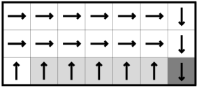
The Cliffwalk is a $3\times 7$ grid world. The top-left corner is initial state, top-right corner is goal state with reward of $10$ , and other states in first row are terminal states with reward of $-10$ . There is a penalty of $-1$ in all other states. The agent has four actions: UP( $0$ ), RIGHT( $1$ ), DOWN( $2$ ), and LEFT( $3$ ). Each action has $90\%$ chance to successfully move, but with probability of $10\%$ one of the other three directions is randomly chosen and the agent moves in that direction. If the agent attempts to get out of the boundary, it will stay in place. Optimal and non optimal poilcies of Cliffwalk used in experiments are as follows:

Optimal policy: $[2,0,0,0,0,0,0,2,2,2,2,2,1,0,1,1,1,1,1,1,0]$

Non optimal policy: $[0,0,2,1,2,1,2,1,0,2,0,3,2,0,3,1,0,1,1,1,3]$

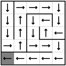
Maze

The Maze is a $5\times 5$ grid world with $16$ walls. The top-left corner is the initial state, and the bottom-left corner is the goal state with reward of $10$ . Similar to the Clifffwalk, there is a penalty of $-1$ in all other states, and the agent has four actions: UP( $0$ ), RIGHT( $1$ ), DOWN( $2$ ), and LEFT( $3$ ). Each action has $90\%$ chance to successfully move but with probability of $10\%$ one of the other three directions is randomly chosen and the agent moves in that direction. If the agent attempts to get out of the boundary or hits a wall, it will stay in place. Optimal and non optimal poilcies of Maze used in experiments are as follows:

Optimal policy: $[2,1,1,1,2,2,0,2,3,2,2,0,2,0,3,1,0,1,1,2,0,3,3,3,3]$

Non optimal policy: $[2,2,3,0,3,0,2,1,3,2,2,2,3,3,1,0,3,0,3,3,3,3,1,1,0]$

Chain Walk

We use the Chain Walk environment, as described by Farahmand and Ghavamzadeh [2021], which is similar to the formulation by Lagoudakis and Parr [2003]. Chain Walk is parametrized by the tuple $(|\mathcal{X}|,|\mathcal{A}|,b_{p},b_{r})$ . It is circular chain, where the state $1$ and $50$ are connected. The reward is state-dependent. State $3$ is goal state with reward $1$ , state $50$ gives reward $-1$ , and all other states give reward $0$ . Agent has two actions: RIGHT( $0$ ) and LEFT( $1$ ). Each action has $80\%$ chance to successfully move but with probability of $40/3\%$ agent will stay in place, and with probability of $20/3\%$ agent will move opposite direction. Optimal poilcy of Chain Walk used in experiments is as follows:

Optimal policy: $[0,0,0,1,1,1,1,1,1,1,1,1,1,1,1,1,1,1,1,1,1,1,1,1,1,1,1,1,1,0,0,0,0,0,0,0,0,0,$ $0,0,0,0,0,0,0,0,0,0,0,0]$

Non optimal policy: $[1,0,0,1,1,1,1,1,1,1,0,1,0,0,0,0,0,0,1,1,1,1,1,1,0,1,1,1,0,0,0,1,1,1,1,1,$

$0,0,1,1,0,1,0,0,1,1,0,0,1,0]$ , $[0,1,1,0,1,1,0,0,1,1,0,1,1,1,1,0,1,1,1,0,0,0,0,0,1,1,1,1,1,1,1,$

$1,1,1,1,1,1,0,0,1,0,0,1,0,1,0,1,0,1,1]$

Garnet

We use the Garnet environment as described by Farahmand and Ghavamzadeh [2021], Rakhsha et al. [2022], which is based on Bhatnagar et al. [2009]. Garnet is parameterized by the tuple $(|\mathcal{X}|,|\mathcal{A}|,b_{p},b_{r})$ . $|\mathcal{X}|$ and $|\mathcal{A}|$ are the number of states and actions, and $b_{p}$ is the branching factor of the environment, which is the number of possible next states for each state-action pair. We randomly select $b_{p}$ states without replacement and then, transition distribution is generated randomly. We select $b_{r}$ states without replacement, and for each selected $x$ , we assign state-dependent reward a uniformly sampled value in $(0,1)$ .

11. Rank- $1$ DDVI for Control Experiments

In this experiment, we consider Chain Walk and Garnet. We use Garnet with 100 states, 8 actions, a branching factor of 6, and 10 non-zero rewards throughout the state space. We use normalized errors $\|V^{k}-V^{\pi}\|_{1}/\|V^{\star}\|_{1}$ , $\gamma=0.995$ , and $E_{1}=\frac{1}{n}\mathbf{1}\mathbf{1}^{\top}$ , where $n$ is the number of states. For Garnet, we plot average values on the 100 Garnet instances and denote one standard error with the shaded area. Figure 7(a) and 7(b) show that rank- $1$ DDVI for Control does indeed provide an acceleration.

12. Additional DDVI Experiments and Details

In all experiments, we set DDVI’s $\alpha=0.99$ . In experiments for Figure 1, the QR iteration is run for 600 iterations. For PID VI, we set $\eta=0.05$ and $\epsilon=10^{-10}$ . In Anderson VI, we have $m=5$ . In Figure 2, we use 20 Garnet mdps with branching factor $b_{p}=3$ , and $b_{r}=0.1*|\mathcal{X}|$ .

We perform further comparison of convergence in Figures 8, 9, 10, 11. Figure 8 is run with Garnet environment with $50$ states and $40$ branching factor that matches the setting in [Goyal and Grand-Clément, 2022].

13. DDTD Experiments

A key part of our experimental setup is the model $\hat{\mathcal{P}}$ . To show the robustness of DDTD to model error and also its advantage over Dyna, we consider the scenario that $\hat{\mathcal{P}}$ has some non-diminishing error. We achieve this with the same technique as [Rakhsha et al., 2022]. Assume that each iteration $t$ , the empirical distribution of the next state from $x,a$ is $\mathcal{P}_{\mathrm{MLE}}(\cdot|x,a)$ , which is going to be updated with every sample. For some hyperparameter $\theta\in[0,1]$ , we set the approximate dynamics $\hat{\mathcal{P}}(\cdot|x,a)$ as

\displaystyle\hat{\mathcal{P}}(\cdot|x,a)=(1-\theta)\cdot\mathcal{P}_{\mathrm{MLE}}(\cdot|x,a)+\theta\cdot U(\{x^{\prime}|\mathcal{P}_{\mathrm{MLE}}(x^{\prime}|x,a)>0\})

(10)

where $U(S)$ for $S\subseteq\mathcal{X}$ is the uniform distribution over $S$ . The hyperparameter $\theta$ controls the amount of error introduced in $\hat{\mathcal{P}}$ . If $\theta=0$ , we have $\hat{\mathcal{P}}=\mathcal{P}_{\mathrm{MLE}}$ which becomes arbitrarily accurate with more samples. With larger $\theta$ , $\hat{\mathcal{P}}(\cdot|x,a)$ will be smoothed towards the uniform distribution more, which leads to a larger model error. In Dyna, we keep the empirical average of past rewards for each $x,a$ in $\hat{r}\colon\mathcal{X}\times\mathcal{A}\to\mathbb{R}$ and perform planning with $\hat{\mathcal{P}},\hat{r}$ at each iteration to calculate the value function, that is $V=(I-\gamma\hat{\mathcal{P}}^{\pi})^{-1}\hat{r}^{\pi}$ . In Figure 3, we have shown the result for $\theta=0.3$ . In Figure 12 and Figure 13 we show the results for $\theta=0.1,0.3,0.5$ in both Maze and Chain Walk environments.

As we see in Figure 12 and Figure 13, DDTD shows a faster convergence than the conventional TD. In Maze, this is only achieved with higher rank versions of DDTD but in Chain Walk, even rank-1 DDTD is able to significantly accelerate the learning. Also note that unlike Dyna, DDTD is converging to the true value function despite the model error. We observe that the impact of model error on DDTD is very mild. In some cases such as rank-3 DDTD in Maze, between $\theta=0.3$ and $\theta=0.5$ , we observe slightly slower convergence with higher model error. The hyperparamaters of TD Learning and DDTD are given in Table 1 and 2.

Table 1: Hyperparamters for the Maze environment. Cells with multiple values provide the value of the hyperparameter for

\theta=0.1

\theta=0.3

, and

\theta=0.5

, respectively.

	rank-1 DDTD	rank-2 DDTD	rank-3 DDTD	rank-4 DDTD	TD
$\eta$ (learning rate)	$0.3,0.3,0.3$	$0.3,0.3,0.3$	$0.07,0.07,0.07$	$0.07,0.07,0.07$	0.3
$\alpha$	$0.8,0.8,0.8$	$0.7,0.8,0.8$	$0.9,0.9,0.9$	$0.9,0.9,0.9$	-
$K$	10	10	10	10	-

Table 2: Hyperparamters for the Chainwalk environment. Cells with multiple values provide the value of the hyperparameter for

\theta=0.1

\theta=0.3

, and

\theta=0.5

, respectively.

	rank-1 DDTD	rank-2 DDTD	rank-3 DDTD	rank-4 DDTD	TD
learning rate ( $\eta$ )	1	1	1	1	1
$\alpha$	$0.9,0.9,0.9$	$0.9,0.8,0.8$	$0.9,0.8,0.8$	$0.9,0.8,0.8$	-
$K$	10	10	10	10	-

	$\displaystyle\\|V^{k}-V^{\star}\\|$	$\displaystyle=\left\\|\gamma^{k}\left(I+\frac{\gamma}{1-\gamma}\mathbf{1}v^{\top}\right)\left(\mathcal{P}^{\pi^{\star}}-E_{1}\right)^{k-K}\prod_{i=1}^{K}\left({\mathcal{P}^{\pi_{i}}-E_{1}}\right)(V^{0}-V^{\star})\right\\|$
		$\displaystyle=C\gamma^{k}\left\\|\left(\mathcal{P}^{\pi^{\star}}-E_{1}\right)^{k-K}\right\\|\\|V^{0}-V^{\star}\\|$
		$\displaystyle=\tilde{O}(\|\gamma\lambda_{2}\|^{k}\\|V^{0}-V^{\star}\\|)$

Deflated Dynamics Value Iteration

Abstract

1. Introduction

2. Background

Markov Decision Process.

Value Iteration.

Power Iteration.

QR iteration.

3. Deflated Dynamics Value Iteration

3.1. Matrix Deflation

Fact 1 (Hotelling’s deflation, [Meirovitch, 1980, Section 5.6]).

Fact 2 (Wielandt’s deflation, [Soto and Rojo, 2006, Theorem 5]).

Fact 3 (Schur deflation, [Saad, 2011, Proposition 4.2]).

3.2. Matrix Splitting: SOR

3.3. Deflated Dynamics Value Iteration

Theorem 3.1.

Corollary 3.2.

4. Computing Deflation Matrix EE

4.1. Rank-11 DDVI for PE and Control

Theorem 4.1.

Discussion.

4.2. DDVI with Automatic Power Iteration

Rank-ss DDVI with the QR Iteration.

5. Deflated Dynamics Temporal Difference Learning

Theorem 5.1.

Theorem 5.2.

5.1. Implementation of DDTD

6. Experiments

DDVI with AutoPI, AutoQR, different fixed ranks.

DDVI and other baselines.

Rank-ss DDTD with QR iteration.

7. Conclusion

Acknowledgements

References

Appendix

7.1. Prior works

Acceleration in RL.

Matrix deflation.

Matrix splitting of value iteration.

Convergence analysis of TD learning

8. Proof of Theoretical Results

8.1. Proof of Theorem 3.1

8.2. Proof of Collorary 3.2

8.3. Proof of Theorem 4.1

8.4. Proof of Theorem 5.1

Proposition 8.1.

8.5. Proof of Theorem 5.2

Proposition 8.2.

8.6. Non-asymptotic convergence analysis of DDTD

Proposition 8.3.

Theorem 8.4 (DDTD with constant stepsize).

Theorem 8.5 (DDTD with diminishing stepsize).

9. DDVI with QR Iteration, AutoPI and AutoQR

9.1. DDVI with QR Iteration

9.2. DDVI with AutoPI and AutoQR

10. Environments

Cliffwalk

Maze

Chain Walk

Garnet

11. Rank-11 DDVI for Control Experiments

12. Additional DDVI Experiments and Details

13. DDTD Experiments

4. Computing Deflation Matrix $E$

4.1. Rank- $1$ DDVI for PE and Control

Rank- $s$ DDVI with the QR Iteration.

Rank- $s$ DDTD with QR iteration.

11. Rank- $1$ DDVI for Control Experiments