Defocusing Hirota equation with fully asymmetric non-zero boundary conditions: the inverse scattering transform

It will be convenient to define some notations:

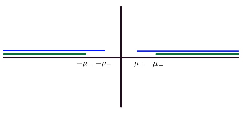
As $x\to\pm\infty$, the branch points are the values of $z$ for which $\lambda_{\pm}=0$, i.e. $z=\pm\mu_{\pm}$. We take the branch cuts on $\Xi_{\pm}$ (see Fig. 1). We define $\lambda_{\pm}$ as analytic functions for all $z\in\mathbb{C}\backslash\Xi_{\pm}$, and these functions remain continuous as $z$ approaches $\Xi_{\pm}$ from above. We see that Im$\lambda_{\pm}\geq 0$ and Im$(\lambda_{\pm}\pm z)\geq 0$ for all $z\in\mathbb{C}$. Clearly, $\Xi_{-}\subset\Xi_{+}$ and $\lambda_{\pm}\in\mathbb{R}$, $\forall$ $z\in\Xi_{-}$. Thus, continuous spectrum of the scattering problem consists of $z\in\Sigma_{-}$.

Similarly to [21], the eigenvector matrices of $U_{\pm}$ can be expressed as follows:

For $z\in\mathring{\Xi}_{\pm}$, we introduce the Jost solutions $\Psi_{\pm}(x,t,z)$ by

Let

where

We introduce the the modified eigenfunctions

It is evident that

One can formally integrate the ODE for $v_{\pm}$ to obtain

where $\hbox{e}^{\alpha\hat{\sigma}_{3}}A:=\hbox{e}^{\alpha\sigma_{3}}A\hbox{e}^{-\alpha\sigma_{3}}$ and $\Delta P_{\pm}(x,t):=P(x,t)-P_{\pm}(t)$.

Let $v_{\pm}=(v_{\pm,1},v_{\pm,2})$. Using the standard Neumann iteration for (2.15), we can prove that if $p(x,t)-p_{\pm}(t)\in L^{1}(\mathbb{R}^{\pm})$, then $v_{-,2}$ is analytic in $\mathbb{C}\backslash\Xi_{-}$, whereas $v_{+,1}$ is analytic in $\mathbb{C}\backslash\Xi_{+}$. In addition, for $t\geq 0$, when $(1+|x|)(p(x,t)-p_{\pm}(t))\in L^{1}(\mathbb{R}^{\pm})$, (2.15) are well-defined when $z\to\pm\mu_{\pm}$. We can see that $v_{-}$ and $v_{+}$ admit the form as $z\to\pm\mu_{-}$ and $z\to\pm\mu_{+}$, respectively,

Using tr$U=0$ and Abel’s formula, we find that $\hbox{det}\Psi_{\pm}$ is independent of $x$. Evaluate $\hbox{det}\Psi_{\pm}$ as $x\to\pm\infty$ to obtain

Since both $\Psi_{\pm}$ solve the scattering problem for $z\in\mathring{\Xi}_{-}$, one has

with

It is mentioned that $S$ is independent of $x$. From (2.19), we have $\hbox{det}S\neq 1$, which is a significant distinction from the case of symmetric NZBCs [21]. Let $S(z,t)=(s_{ij}(z,t))_{1\leq i,j\leq 2}$. Using (2.18), $s_{ij}$ $(i,j=1,2)$ can be expressed as follows:

From (2.20), it is shown that $s_{22}$ is analytic for $z\in\mathbb{C}\backslash\Xi_{+}$. Because $\Psi_{-,2}$ can be extended analytically to $z\in\mathbb{C}\backslash\Xi_{-}$, $\Psi_{+,1}$ and $\Psi_{+,2}$ are defined on $\Xi_{+}$, we may extend the definitions of $s_{12}$ and $s_{22}$ pointwise to $\mathring{\Xi}_{+}$. Since $d_{+}$ has a double zero at $z=\pm\mu_{+}$, $s_{12}$ and $s_{22}$ are singular at $z=\pm\mu_{+}$ .

It will be useful to introduce the reflection coefficients

which will be needed in the following discussions.

Due to the involutions $z\mapsto z^{*}$ and $\lambda_{\pm}(z)\mapsto-\lambda_{\pm}(z)$, we have the two kinds of symmetries.

(i) The first symmetry follows from $z\mapsto z^{*}$. It can be directly verified that $\sigma_{1}\Psi^{*}(x,t,z^{*})\sigma_{1}$ also satisfies the scattering problem and demonstrates identical asymptotic behavior to $\Psi(x,t,z)$ as $x\to\pm\infty$, where

Hence, we have

Combining the (2.18) and (2.22), we have the following symmetry relation

which yields

and

It follows from (2.19) and (2.24) that

From $d_{-}/d_{+}>0$ for $z\in\mathring{\Xi}_{-}$, we see that $s_{22}$ has no zeros on $z\in\mathring{\Xi}_{-}$.

Next, we consider $z\mapsto z^{*}$ for $z\notin\Sigma_{+}$. One can verify that if $\Psi(x,t,z)$ satisfies the scattering problem, then $\sigma_{1}\Psi^{*}(x,t,z^{*})$ also satisfies it. Taking the limit $x\to-\infty$, we have

Similarly, take the limit as $x\to\infty$ to obtain

Using the formula (2.20), we find that

(ii) The second symmetry arises from an alternative selection of $\lambda_{\pm}(z)$, i.e. $\lambda_{\pm}(z)\mapsto-\lambda_{\pm}(z)$. To prevent any confusion caused by notation, we denote

It is worth noting that this choice does not affect the formal independence of the integral equations for the eigenfunctions. If $\Psi_{\pm}(x,t,z,\lambda_{\pm}(z))$ represents the solution to the scattering problem, it follows that $\hat{\Psi}_{\pm}(x,t,z):=\Psi_{\pm}(x,t,z,\hat{\lambda}_{\pm}(z))$ is also a valid solution.

From (2.9) and (2.10), we define the Jost solutions $\hat{\Psi}_{\pm}(x,t,z)$ admit the following asymptotic behavior

Since $\Psi_{\pm}$ and $\hat{\Psi}_{\pm}$ are matrix solutions for the first part of the (2.1) for all $z\in\mathring{\Xi}_{\pm}$, we express

Define $\hat{S}(z,t)$ as the scattering matrix for $\hat{\Psi}_{\pm}$. Following direct calculations, we have

Thus, elements in $S$ are simply related to elements in $\hat{S}$ as

According to the definition of $\lambda_{\pm}$, it is clear that $\lambda_{\pm}$ are defined to be continuous as $z\to\Xi_{\pm}$ from above, i.e.

And, $\lambda_{\pm}^{-}$ as $z\to\Xi_{\pm}$ from below, are given by

Using the definition (2.13) and analytical properties of $v_{-,2}$ and $v_{+,1}$, we see that $\Psi_{-,2}$ is analytic for $z\in\mathbb{C}\backslash\Xi_{-}$ and exhibits continuity towards $\Xi_{-}$ from above, and $\Psi_{+,1}$ is analytic for $z\in\mathbb{C}\backslash\Xi_{+}$ and exhibits continuity towards $\Xi_{+}$ from above. On the other hand, $\Psi_{-,2}$ and $\Psi_{+,1}$ as $z\to\Xi_{\pm}$ from below, are given by

Using the relation (2.32), we have

From above relations, we get the limits of $s_{22}$ as $z\to\Xi_{\pm}$ from below:

Recall that $\Psi_{-}$ is well-defined as $z\to\pm\mu_{-}$ and $\Psi_{+}(x,t,\pm\mu_{-})$ solves the scattering problem, we see immediately that the scattering coefficients $s_{ij}$ are well defined at $z=\pm\mu_{-}$. When $z=\pm\mu_{-}$, $d_{-}(z)=0$. It follows that det$S(\pm\mu_{-},t)=0$ and the columns of $\Psi_{-}(x,t,\pm\mu_{-})$ are linearly dependent. By utilizing the asymptotics of $\Psi_{-}(x,t,\pm\mu_{-})$ as well as Wronskian definitions (2.20), we have

Then in view of the expressions (2.24) and (2.40), we find that

From (2.21), we have

Next, we consider $z\to\pm\mu_{+}$. From the definitions and properties of $\Psi_{\pm}$ as well as the Wronskian relations (2.20), we find that only scattering coefficients $s_{22}$ and $s_{12}$ are defined for $z\in\mathring{\Xi}_{\circ}$. Since $d_{+}$ has a double zero at $z=\pm\mu_{+}$, $s_{22}$ and $s_{12}$ have a double pole as $z\to\pm\mu_{+}$. Specifically, we obtain the limits of $s_{22}$ and $s_{12}$ as $z\to\pm\mu_{+}$:

Notice that

It follows that $|\hat{r}(\pm\mu_{+},t)|=1$.

Following the similar analysis in [33], we conclude that no zeros in the inverse scattering problem for $\mathring{\Xi}_{\circ}$. Specifically,

which shows that $\hat{r}(z,t)$ has no zeros in $\mathring{\Xi}_{\circ}$. In the following, we make the assumption that there exists a finite number of zeros of $s_{22}(z,t)$ lie in $(-\mu_{+},\mu_{+})$. This condition is satisfied if $s_{22}(\pm\mu_{+},t)\neq 0$.

Let $z_{1},\cdots,z_{W}$ represent the zeros of $s_{22}(z,t)$ in $(-\mu_{+},\mu_{+})$. At $z=z_{l}$, we get

where $b_{l}$ is a scalar independent of $x$ and $z$. Now, we define the norming constants

where ^′ indicates the derivative with respect to $z$.

From (2.27), (2.28) and (2.29), one can derive the following relations:

and

which yields

References

- [1] V. E. Zakharov, A. B. Shabat, Exact theory of two-dimensional self-focusing and one-dimensional self-modulation of waves in nonlinear media, Sov. Phys. JETP 34, 62–69 (1972).
- [2] G. Biodini, G. Kovai, Inverse scattering transform for the focusing nonlinear Schrdinger equation with nonzero boundary conditions, J. Math. Phys. 55, 031506 (2014).
- [3] V. E. Zakharov, A. B. Shabat, Interaction between solitons in a stable medium, Sov. Phys. JETP 37, 823–828 (1973).
- [4] F. Demontis, B. Prinari, C. van der Mee, F. Vitale, The inverse scattering transform for the defocusing nonlinear Schrdinger equations with nonzero boundary conditions, Stud. Appl. Math. 131(1), 1-40 (2013).
- [5] J. P. Wu, X. G. Geng, Inverse scattering transform of the coupled Sasa–Satsuma equation by Riemann–Hilbert approach, Commun. Theor. Phys. 67(5), 527 (2017).
- [6] W. X. Ma, Sasa–Satsuma type matrix integrable hierarchies and their Riemann–Hilbert problems and soliton solutions, Phys. D 446, 133672 (2023).
- [7] B. Yang, Y. Chen Y, High-order soliton matrices for Sasa–Satsuma equation via local Riemann–Hilbert problem, Nonlinear Anal-Real 45, 918-941 (2019).
- [8] D. J. Kaup, A. C. Newell, An exact solution for a derivative nonlinear Schrdinger equation, J. Math. Phys. 19(4), 798–801 (1978).
- [9] G. Q. Zhou, N. N. Huang, An -soliton solution to the DNLS equation based on revised inverse scattering transform, J. Phys. A: Math. Theor. 40(45), 13607 (2007).
- [10] T. Kawata, H. Inoue, Exact solutions of the derivative nonlinear Schrdinger equation under the nonvanishing conditions, J. Phys. Soc. Jpn. 44(6), 1968–1976 (1978).
- [11] X. J. Chen, W. K. Lam, Inverse scattering transform for the derivative nonlinear Schrdinger equation with nonvanishing boundary conditions, Phys. Rev. E 69(6), 066604 (2004).
- [12] G. Q. Zhang, Z. Y. Yan, Inverse scattering transforms and -double-pole solutions for the derivative NLS equation with zero/non-zero boundary conditions. arXiv preprint arXiv:1812.02387, 2018.
- [13] C. S. Gardner, J. M. Greene, M. D. Kruskal, R.M. Miura, Method for solving the Korteweg-de Vries equation, Phys. Rev. Lett. 19, 1095–1097 (1967).
- [14] M. Wadati, The modified Korteweg-de Vries equation, J. Phys. Soc. Japan 34, 1289–1296 (1973).
- [15] M. Wadati, K. Ohkuma, Multiple-pole solutions of the modified Korteweg-de Vries equation, J. Phys. Soc. Japan 51, 2029–2035 (1982).
- [16] F. Demontis, Exact solutions of the modified Korteweg–de Vries equation, Theoret. Math. Phys. 168, 886 (2011).
- [17] G. Q. Zhang, Z. Y. Yan, Focusing and defocusing mKdV equations with nonzero boundary conditions: Inverse scattering transforms and soliton interactions, Phys. D 410, 132521 (2020).
- [18] D. E. Baldwin, Dispersive shock wave interactions and wwo-dimensional ocean-wave soliton interactions (Ph.D. thesis), University of Colorado, 2013.
- [19] B. Prinari, M. J. Ablowitz, G. Biondini, Inverse scattering transform for the vector nonlinear Schrdinger equation with nonvanishing boundary conditions, J. Math. Phys. 47(6), 063508 (2006).
- [20] X. Zhang, S. Tian, J. Yang, Inverse scattering transform and soliton solutions for the Hirota equation with distinct arbitrary order poles, Adv. Appl. Math. Mech. 14(4), 893-913 (2022).
- [21] G. Zhang, S. Chen, Z. Yan, Focusing and defocusing Hirota equations with non-zero boundary conditions: Inverse scattering transforms and soliton solutions, Commun. Nonlinear Sci. 80, 104927 (2020).
- [22] W. X. Ma, Sasa-Satsuma type matrix integrable hierarchies and their Riemann-Hilbert problems and soliton solutions, Phys. D 446, 133672 (2023).
- [23] W. X. Ma, Riemann-Hilbert problems and inverse scattering of nonlocal real reverse-spacetime matrix AKNS hierarchies, Phys. D 430, 133078 (2022).
- [24] G. Q. Zhang, Z. Y. Yan, The derivative nonlinear Schrdinger equation with zero/nonzero boundary conditions: Inverse scattering transforms and -double-pole solutions, J. Nonlinear Sci. 30(6), 3089-3127 (2020).
- [25] Z. C. Zhang, E. G. Fan, Inverse scattering transform for the Gerdjikov–Ivanov equation with nonzero boundary conditions. Z. Angew. Math. Phys. 71, 149 (2020).
- [26] G. Biondini, D. Kraus, Inverse scattering transform for the defocusing Manakov system with nonzero boundary conditions, SIAM J. Math. Anal. 47(1), 706-757 (2015).
- [27] M. J. Ablowitz, G. Biondini, B. Prinari, Inverse scattering transform for the integrable discrete nonlinear Schrdinger equation with nonvanishing boundary conditions, Inverse Probl. 23(4), 1711 (2007).
- [28] X. J. Chen, W. K. Lam, Inverse scattering transform for the derivative nonlinear Schrdinger equation with nonvanishing boundary conditions, Phys. Rev. E 69, 066604 (2004).
- [29] Y. D. Zhuang, Y. Zhang, H. Y. Zhang, P. Xia, Multi-soliton solutions for the three types of nonlocal Hirota equations via Riemann–Hilbert approach, Commun. Theor. Phys. 74(11), 115004 (2022).
- [30] X. T. Chen, Y. Zhang, J. L. Liang, R. Wang, The -soliton solutions for the matrix modified Korteweg–de Vries equation via the Riemann–Hilbert approach, Eur. Phys. J. Plus 135, 1-9 (2020).
- [31] M. Boiti, F. Pempinelli, The spectral transform for the NLS equation with left–right asymmetric boundary conditions, Nuovo Cimento A 69, 213–227 (1982).
- [32] F. Demontis, B. Prinari, C. Van Der Mee, F. Vitale, The inverse scattering transform for the focusing nonlinear Schrdinger equation with asymmetric boundary conditions, J. Math. Phys. 55(10), 101505 (2014).
- [33] G. Biondini, E. Fagerstrom, B. Prinari, Inverse scattering transform for the defocusing nonlinear Schrdinger equation with fully asymmetric non-zero boundary conditions, Phys. D 333, 117-136 (2016).
- [34] R. Hirota, Exact envelope-soliton solutions of a nonlinear wave equation, J. Math. Phys. 14, 805–809 (1973).
- [35] J. Kim, Q. H. Park, H. J. Shin, Conservation laws in higher-order nonlinear Schrdinger equations. Phys. Rev. E 58, 6746–6751 (1998).
- [36] L. J. Li, Z. W. Wu, L. H. Wang, J. S. He, High-order rogue waves for the Hirota equation, Ann. Phys. 334, 198-211 (2013).
- [37] Z. Du, X. H. Zhao, Vector localized and periodic waves for the matrix Hirota equation with sign-alternating nonlinearity via the binary Darboux transformation, Phys. Fluids 35, 075108 (2023).
- [38] C. Q. Dai, J. F. Zhang, New solitons for the Hirota equation and generalized higher-order nonlinear Schrdinger equation with variable coefficients, J. Phys. A: Math. Theor. 39(4), 723 (2006).
- [39] Y. S. Tao, J. S. He, Multisolitons, breathers, and rogue waves for the Hirota equation generated by the Darboux transformation, Phys. Rev. E 85(2), 026601 (2012).
- [40] D. S. Wang, F. Chen, X. Y. Wen, Darboux transformation of the general Hirota equation: multisoliton solutions, breather solutions, and rogue wave solutions, Adv. Diff. Equ. 2016(1), 1-17 (2016).
- [41] S. Y. Chen, Z. Y. Yan, B. L. Guo, Long-time asymptotics for the focusing Hirota equation with non-zero boundary conditions at infinity via the Deift-Zhou approach, Math. Phys. Anal. Geom. 24(2), 17 (2021).
- [42] L. Huang, The initial-boundary-value problems for the Hirota equation on the half-line, Chin. Ann. Math. Ser. B 41(1), 117–132 (2020).
- [43] X. E. Zhang, L. M. Ling, Asymptotic analysis of high-order solitons for the Hirota equation, Phys. D 426, 132982 (2021).
- [44] J. Cen, A. Fring, Asymptotic and scattering behaviour for degenerate multi-solitons in the Hirota equation, Phys. D 397, 17-24 (2019).
- [45] B. Prinari, F. Vitale, Inverse scattering transform for the focusing nonlinear Schrdinger equation with one-sided nonzero boundary condition, Cont. Math. 651, 157-194 (2015).