Delay-sensitive Task Offloading in Vehicular Fog Computing-Assisted Platoons
Abstract
Vehicles in platoons need to process many tasks to support various real-time vehicular applications. When a task arrives at a vehicle, the vehicle may not process the task due to its limited computation resource. In this case, it usually requests to offload the task to other vehicles in the platoon for processing. However, when the computation resources of all the vehicles in the platoon are insufficient, the task cannot be processed in time through offloading to the other vehicles in the platoon. Vehicular fog computing (VFC)-assisted platoon can solve this problem through offloading the task to the VFC which is formed by the vehicles driving near the platoon. Offloading delay is an important performance metric, which is impacted by both the offloading strategy for deciding where the task is offloaded and the number of the allocated vehicles in VFC to process the task. Thus, it is critical to propose an offloading strategy to minimize the offloading delay. In the VFC-assisted platoon system, vehicles usually adopt the IEEE 802.11p distributed coordination function (DCF) mechanism while having various computation resources. Moreover, when vehicles arrive and depart the VFC randomly, their tasks also arrive at and depart the system randomly. In this paper, we propose a semi-Markov decision process (SMDP) based offloading strategy while considering these factors to obtain the maximal long-term reward reflecting the offloading delay. Our research provides a robust strategy for task offloading in VFC systems, its effectiveness is demonstrated through simulation experiments and comparison with benchmark strategies.
Index Terms:
Platoons, vehicular fog computing, offloading, delay.I Introduction
With the development of autonomous driving technology, platoons have been widely studied to improve the road safety. A platoon is composed of several autonomous driving vehicles such as a leader vehicle and other member vehicles. The leader vehicle controls the velocity, acceleration and driving direction of the platoon. The member vehicles along the same lane follow the leader vehicle one by one [1, 2]. The on-board equipments of vehicles in the platoon such as radar and lidar collect a large amount of data to support various real-time vehicular applications such as automatic navigation, multimedia entertainment, high definition (HD) map and precise positioning[3, 4, 5, 6]. These data are usually redundant and thus vehicles in the platoon could compute and analyze the data to extract useful information. Therefore, vehicles in platoons may have many tasks to deal with.
When a task arrives at a vehicle in a platoon, the vehicle may not be able to process the arrived task due to its limited computation resource. In this case, it usually offloads the task to the other vehicles in the platoon for assistant processing, whose result can be sent back to the vehicle. However, when the computation resources of the platoon are still insufficient, the task cannot be processed in time by offloading to the platoon. We have utilized a vehicular fog computing (VFC)-assisted system to tackle this problem, where the VFC is formed by the personal vehicles near the platoon. In VFC-assisted platoon, one vehicle is able to request to offload tasks to the VFC to assist the platoon for processing [7, 8, 9]. When the requested vehicle offloads a task to the VFC, it transmits the task to the leader vehicle. Afterwards, the system determines how many vehicles in the VFC to process and then the leader vehicle divides the task into the corresponding number of subtasks. Then the leader vehicle transmits the subtasks to the corresponding vehicles in the VFC one by one. After that the vehicles process the assigned subtasks and send back the computing result to the leader vehicle who further forwards the computing result to the requested vehicle.
Offloading delay is an important metric for the autonomous vehicles in the VFC-assisted platoon system [10]. If the offloading delay is large, the requested vehicle in the platoon would take a long time to receive the result, resulting in unsatisfying the requirements of vehicular applications. The offloading delay includes transmitting delay, computing delay, and backhaul delay. In fact, transmitting delay represents the time that the requested vehicle transmits the task to other vehicles for assistant processing; computing delay represents the time that the vehicles process the task and the backhaul delay is the time that vehicles send back the computing result. The offloading delay is impacted by both the locations where tasks are offloaded and the number of vehicles allocated for task processing. On the one hand, determining the place where the task is offloaded will affect the offloading delay. Specifically, offloading the task to the VFC will incur a higher transmitting delay, while the VFC can provide more computation resources to process the task, which would cause a lower computing delay. Offloading the task to the platoon will incur a lower transmitting delay, while the computation resources in the platoon are limited, which would cause a higher computing delay. Hence, it is important to determine where the task is offloaded to minimize the offloading delay. On the other hand, the number of the allocated vehicles in VFC to process the task will also affect the offloading delay. Specifically, if more vehicles are chosen for offloading, the sufficient computation resources reduce the computing delay, while more subtasks would be divided and transmitted to the vehicles in the VFC in turn, which increases the transmitting delay. Hence, it is another important problem to determine how many vehicles in the VFC to process tasks to minimize the offloading delay. As far as we know, there is no work to design a task offloading strategy in the VFC-assisted platoon, which motivates us to conduct this work.
In the VFC-assisted platoon system, vehicles usually adopt the IEEE 802.11p distributed coordination function (DCF) mechanism to offload tasks [11, 12, 13, 14, 15]. The computation resources of vehicles in the platoon are usually different. Meanwhile, tasks arrive and depart the system randomly, and the vehicles also arrive and depart the VFC randomly. These factors pose challenges to design the optimal offloading strategy to obtain the maximal the long-term reward related to offloading delay of the system. This paper jointly considers the 802.11p DCF mechanism and some factors, i.e., heterogeneous computation resource of vehicles in the platoon, the random task arrival and departure as well as the random arrival and departure of vehicles in the VFC, to design an semi-Markov decision process (SMDP) based offloading strategy by maximizing the long-term reward in the VFC-assisted platoon. The main contributions of this paper are summarized as follows.
-
1)
We propose an offloading strategy for a VFC-assisted platoon system. This strategy takes into account several factors, i.e., the heterogeneous computation resources of vehicles in the platoon, the random arrival and departure of task, the random arrival and departure of the vehicles in the VFC, and the 802.11p DCF mechanism.
-
2)
We adopt the SMDP to model the task offloading process and design the SMDP framework including state, action, reward and transition probability, where the transmitting delay is derived according to the 802.11p DCF mechanism to determine the reward.
-
3)
We propose an iterative algorithm to solve the SMDP model to obtain the optimal offloading strategy. Extensive experiments demonstrated that the proposed offloading strategy outperforms the baseline strategy.
The rest of this paper is organized as follows. Section II reviews the related work. Section III describes the system model briefly. Section IV sets up the SMDP framework to model the offloading process in VFC-assisted platoon. Section V solves the SMDP model by an iterative algorithm. Section VI presents the simulation results. Section VII concludes this paper.
II Related Work
In this section, we review the state-of-art works on the offloading in platoons and offloading in VFC.
II-A Task offloading in platoons
In recent years, some works designed the task offloading strategy in platoon to optimize various performances. In [16], Fan et al. designed the task offloading strategy in the mobile edge computing (MEC)-assisted platoon. They adopted the directed acyclic graph to model the task offloading process, and then employed the Lagrangian relaxation-based aggregated cost (LARAC) algorithm to minimize the cost of the task offloading. In [17], Ma et al. considered the change of vehicle velocity in the platoon and proposed a task offloading and task take-back strategy. The reinforcement learning is adopted to enhance the offloading efficiency and avoid the link disconnection resulting from task processing failures. In [18], Hu et al. designed the task offloading strategy in the MEC -assisted platoon under the stable condition of task queues. The Lyapunov optimization algorithm is employed to reduce the energy consumption of task execution and improve the offloading efficiency considering transmitting delay as well as computing delay. In [19], Du et al. considered the sensing, computation, communication and storage resources of a single autonomous vehicle and proposed a communication strategy for autonomous driving platoon. In addition, they adopted the genetic algorithm to design the offloading strategy to achieve the minimized processing delay. In [20], Zheng et al. proposed a platoon task offloading strategy based on the dynamic non-orthogonal multiple access (NOMA). The long-term energy consumption is minimized by optimizing the allocation of both the communication and computation resource based on the Lyapunov and block successive upper bound minimization (BSUM) methods. In [21], Xiao et al. considered a scenario where the requested vehicle offloads tasks to the vehicles in the platoon and proposed a resource allocation strategy based on the requested vehicle’s service pricing to effectively utilize the resources in the platoon. However, the computation resource in a platoon is limited. When the resources in the platoon are not enough to process the task, a potential threat will be posed for safety. In this situation, the vehicles driving near the platoon may form a VFC to provide computation resource.
II-B Task offloading in VFC
Many works have studied task offloading in the VFC. In [22], Liao et al. considered the uncertain information and designed a task offloading strategy in the VFC to get the minimized total network delay. In [23], Zhou et al. considered a two-stage VFC framework and designed a task offloading strategy according to the price-based matching algorithm to minimize the long-term task offloading delay. In [24], Shi et al. proposed a task offloading strategy, where vehicles are likely to share idle computation resources by dynamic pricing strategy to maximize the utility of offloading tasks. In [25], Yadav et al. considered the vehicular node mobility and end-to-end latency deadline constraints and designed an energy-efficient dynamic computation offloading and resources allocation strategy (ECOS) in the VFC to minimize energy consumption and service latency. In [26], Xie et al. considered the parallel computation task offloading problem in the VFC and proposed an offloading strategy to reduce the service time and improve the amount of the finished tasks by using the hidden Markov model. In [27], Lqbal et al. designed an offloading strategy to improve the performance of queuing delay, end-to-end delay and task completion rate based on the computing capacity and the workload of vehicles in the VFC. In [28], Misra et al. proposed a task offloading strategy in a software-defined VFC network to reduce the task computing delay and minimize the control overhead in the network. In [29], Liu et al. considered the dynamic requirements and resource constraints in the two-layer VFC architecture and proposed a task offloading strategy to maximize the task service rate. In [30], Wang et al. proposed an online learning-based task offloading algorithm in the VFC to minimize the task offloading latency. In [31], Zhu et al. proposed an event-triggered dynamic task allocation framework in the VFC by using linear programming-based optimization and binary particle swarm optimization to minimize average service latency. In [32], Zhao et al. proposed a contract-based incentive mechanism that combines resource contribution and resource utilization in the VFC to improve the quality of service of vehicles. Moreover, they proposed a task offloading strategy based on the queuing model to enhance the performance of task offloading and resource allocation. In [33], Tang et al. considered the task deadline and proposed an offloading strategy in the VFC to enhance the offloading efficiency. In [34], Yang et al. considered the effective time of tasks in the VFC at the crossroads and proposed a low-cost offloading strategy to enhance the offloading efficiency among vehicles. In [35], Mourad et al. considered the intrusion detection tasks in the VFC and proposed a task offloading strategy to minimize the computation execution time and energy consumption and meanwhile maximize the offloading survivability. In [36], Liu et al. considered a two-layer VFC and proposed an adaptive task offloading mechanism to get the maximal tasks’ completion ratio. In [37], Cho et al. adopted the adversarial multi-armed bandit theory to propose an adversarial online learning algorithm with bandit feedback, which aimed to optimize the selection of vehicles in the VFC to minimize the offloading service costs including the delay and energy. In [38], Wu et al. considered directional vehicle mobility to propose a network model to minimize the average response time of the tasks. They further chose the neighboring vehicles to assist to process task based on a greedy algorithm. In [39], Huang et al. jointly considered the task type as well as the velocity of vehicle to propose the task offloading and resource allocation strategy, which decreases the vehicles’ energy cost and increases the income of the vehicles considering the delay constraint. In [40], Alam et al. developed a three-layer generic decentralized cooperative VFC system to overcome the lack of robustness against the high mobility environment. In [41], Fan et al. proposed a joint task offloading and resource allocation strategy for a VFC including devices and vehicles covered by a base station. In [42], Chen et al. focused on a energy-powered multi-server VFC system with cybertwin, where vehicles send the current status of network and unprocessed vehicular application tasks to the macro base station to get the efficient resources allocation. In [43], Chen et al. proposed a distributed multi-hop task offloading model to get a low delay for the task execution in the VFC. In [44], Lin et al. proposed an online task offloading strategy for the unknown dynamics heterogeneous VFC environment based on the online clustering of bandits (CAB) approaches to minimize the expectation of total offloading energy consumption while satisfy stringent delay requirements by learning the relationship between historical observations and rewards. In [45], Liu et al. considered the vehicle mobility and proposed a task offloading strategy by exploiting the computation resources of vehicles in the VFC to get the minimized weighted sum of execution delay as well as computation cost. In [46], Ma et al. proposed a traffic routing-based computation offloading strategy in the cybertwin-driven VFC for vehicle-to-everything applications to reduce latency. However, these works have not considered the platooning scenario.
The works mentioned above show that the strategy of task offloading in VFC has been studied intensively, but for task offloading in the VFC-assisted platoon, to mitigate the limited computation resource, has not been studied. This motivates us to conduct this work. Different from the existing works about task offloading in VFC or platoons, we jointly take into account several factors, i.e., the heterogeneous computation resources of vehicles in the platoon, the random arrival and departure of task, the random arrival and departure of the vehicles in the VFC, and the 802.11p DCF mechanism. Moreover, we adopt the SMDP to model the task offloading process and design the SMDP framework including state, action, reward and transition probability.
III System Model
In this section, we first describe the VFC-assisted system, and then briefly review the IEEE 802.11p DCF mechanism.
III-1 The VFC-assisted platoon
Consider autonomous vehicles in a platoon driving on a lane with the same velocity and a VFC consisting of the personal vehicles within the communication range of the head vehicle of the platoon. The -th vehicle in the platoon is , where is the leader vehicle and are member vehicles. The computing rate of , i.e., central processing unit (CPU) cycles per second, is denoted as . The resource of each vehicle in the VFC is virtualized as a resource unit (RU) [47]. Each RU’s computing rate is the same and denoted as . We consider the computing rate of an autonomous vehicle in the platoon is larger than the computing rate of a RU, thus . The arrival and departure rate of vehicles in the VFC are denoted as and , respectively. The maximum number of vehicles in the VFC system is .
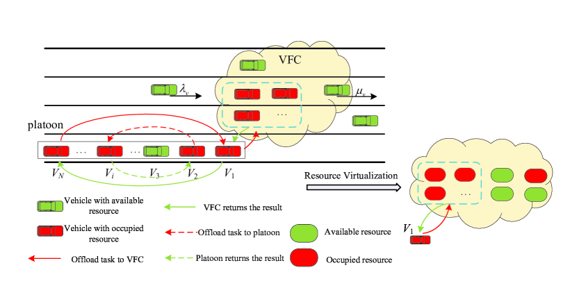

The tasks arrive at each vehicle in the platoon according to the Poisson distribution with arrival rate . When a task arrives at a vehicle in the platoon, the system will make a decision to offload the task to the platoon, VFC, or to discard the task according to the available resources in the platoon and VFC. We consider the following two most general cases, (1) the task can be offloaded to only one vehicle in the platoon due to the sufficient computing rate of each vehicle in the platoon and (2) the task can be offloaded to multiple RUs in the VFC due to the limited computing rate of each RU. Specifically, if the available resources in the platoon are sufficient, the vehicle with the arrival task will request to offload the task to the platoon. Otherwise, the system will check if the VFC has sufficient computation resource and offload the task to it instead. In this case, the requested vehicle first transmits the task to the leader vehicle of the platoon, then the system determines the vehicles in the VFC with available resources to process. The leader vehicle divides the task into the corresponding number of subtasks, and transmits the subtasks to the corresponding vehicles in the VFC one by one. After that each vehicle processes the assigned subtasks to him. Once all the subtasks are executed, the result is sent back to the leader vehicle and further forwarded to the requested vehicle. Note that after the system determines the VFC vehicles, they will not be occupied by other subtasks until all of them have finished the processing. Since the result is of small size, the backhaul delay is significantly small and thus can be neglected [48]. If the available resources are scarce in the platoon and VFC, the system will discard the task. Fig. 1 shows an example for the offloading process including task offloading to platoon and to VFC. The task offloading to platoon in Fig. 1 is described as follows. When a task arrives at in the platoon, and another vehicle in the same platoon has available resource, offloads the task to for processing. After completes processing the task, it returns the result back to . The task offloading to VFC in Fig. 1 is described as follows. When another task arrives at and all the sources of the vehicles in the platoon are occupied. first offloads the task to the leader vehicle in the platoon. Then offloads the task to three RUs in the VFC for processing. After processing, the result is returned to and then returned back to .
In the offloading process, it is assumed that all vehicles in the platoon and VFC communicate with each other within one-hop communication area by adopting the 802.11p DCF mechanism. We will introduce the process of the 802.11p DCF mechanism.
III-2 802.11p DCF mechanism
At the beginning, each vehicle sets the minimum contention window () based on 802.11p DCF mechanism [49]. When a vehicle transmits a task to vehicles, the vehicle will partition the task into sub-tasks. When the vehicle transmits the one sub-task to an allocated vehicle, it first detects the state of the channel. If the channel keeps idle for distributed inter-frame space (DIFS), the vehicle will transmit the sub-task. Otherwise, if the channel is busy, the vehicle will continue to detect the channel state until the channel keeps idle for DIFS. Then a back-off process is initialized to transmit the sub-task. Specifically, the vehicle randomly selects a natural number within for the backoff counter, where is the contention window and is initialized as (i.e., the minimum contention window). The value of the backoff counter is decremented by one if the vehicle detects the idle state in a time slot. The vehicle will transmit the sub-task if the backoff counter is decreased to zero.
The sub-task is transmitted successfully if the vehicle receives an acknowledgment (ACK) after a short inter-frame space (SIFS). If the vehicle has not received an ACK after a specific ACK time out interval, the transmission fails. Then the vehicle will initialize another backoff process to retransmit the sub-task, where the contention window is doubled. If the number of retransmissions does not reach the retransmission limit , the contention window will be doubled to and a new back-off process is initialized for retransmission. Otherwise, if the number of retransmissions reaches the maximum number , the vehicle will discard the sub-task and reset the contention window as to transmit the next sub-task. The following sub-tasks are transmitted sequentially according to the above procedure until all sub-tasks are transmitted successfully. Fig. 2 shows the process that the leader vehicle V1 transmits three sub-tasks to three vehicles (denoted as , and ) in the VFC system.
IV SMDP Framework
In this section, we adopt the SMDP to model the task offloading process in the VFC-assisted platoon system, where the system learns the offloading decision by interacting with the environment in continuous time steps. The duration of each time step follows an exponential distribution. In each step, the system observes the state and then makes an action according to a policy. Afterwards, the system receives a reward which is related to the offloading delay to evaluate the benefit of the system under the state and action. The state transits to the next one according to the state transition probability. After that the system starts the next time step and repeats the above procedures. The target of the SMDP is to find the optimal policy to maximize the long-term reward. Next, we construct the SMDP framework which includes the state set, action set, reward function and state transition probability. For clearity, the notations in this paper are listed in Table I.
| Notation | Description | Notation | Description |
|---|---|---|---|
| Number of vehicles in the platoon. | Number of retransmission. | ||
| The -th vehicle in the platoon. | Vehicles’ arriving /departing rate. | ||
| Task arrival rate. | Maximum number of RUs. | ||
| Required CPU cycles to process each task. | Computing rate of vehicle (CPU cycles per second). | ||
| Computing rate of each RU. | Minimum contention window. | ||
| Maximum number of retransmissions. | A task arrives at the system. | ||
| A task which occupies the resource of departs the system. | A task which occupies RUs departs the system. | ||
| Maximum number of RUs that each task can occupy. | A vehicle arrives at/ departs the VFC. | ||
| The system discards the task. | Vehicle is allocated to process the task. | ||
| The system allocates RUs in the VFC to process the task. | A binary to indicate whether the resource of is occupied. | ||
| Number of the tasks that occupy RUs. | State transition probability of the system. | ||
| Total number of RUs. | Delay that processing the task locally. | ||
| Transmitting delay that a vehicle transmits the task to another vehicle in the platoon. | Transmitting delay that the leader vehicle transmits the task to RUs. | ||
| Saved price of each time unit. | Number of the sub-tasks need to be transmitted. | ||
| Average number of time slots to transmit a task. | Average length of a time slot. | ||
| Number of vehicles in the one-hop communication area when a vehicle transmits a task. | Probability of idle/successful transmission/collision. | ||
| Duration of idle/successful transmission/collision. | Length of a task. | ||
| Propagation delay. | Transmission probability of a vehicle in a time slot. | ||
| Collision probability when a vehicle is transmitting. | Punishment of the system discarding the task/the vehicle which is processing the task departs the system. | ||
| Continuous-time discount factor. |
IV-A State set
The states reflect the resource conditions of the system, which is influenced by the events including a task’s arrival and departure, a vehicle’s arrival and departure in the VFC. Hence, we formulate the states as the resource conditions when different events occur. The state set is formulated as
| (1) |
where () is a binary to indicate whether the resource of is occupied or not, i.e., indicates that the resource of is occupied and indicates that the resource of is available. () is the number of the tasks that occupy RUs, is the maximum number of RUs that each task can occupy, is the total number of RUs in the VFC. Thus, the total number of occupied RUs is calculated as , where is the number of RUs a task occupies, and is the number of the tasks that occupy RUs. Then represents the number of the occupied RUs for the tasks occupied RUs. The total number of occupied RUs should not exceed the total number of RUs in VFC, i.e., . is an event, where denotes that a task arrives at the system, denotes that a task occupying the resource of leaves the system, denotes that a task occupying RUs in the VFC leaves the system, denotes that a vehicle arrives at the VFC, denotes that a vehicle leaves the VFC.
IV-B Action set
The actions reflect the offloading decisions of the system, depending on different events. Specifically, when there is a task arriving, the system will make an offloading decision such as offloading to the platoon, offloading to the VFC or discarding the task, while the system will make no decision when other events occur. Thus, the action set is formulated as
| (2) |
where indicates that vehicle in the platoon is allocated to process the offloaded task, indicates that the system offloads the task to the VFC and allocates total RUs in the VFC to process the task, indicates that the system discards the task. indicates that the system takes no action in the current moment.
IV-C Reward function
The reward function reflects the benefit which is related to the offloading delay under different states and actions. The system will transit from the current state to the next state when an action is taken, thus it gets an income when taking action under state , and incurs a cost during the duration from state to the next state. Hence, the reward function under state and action is calculated as
| (3) |
Next, we will formulate and , respectively.
IV-C1 Income
The state changes when an event occurs. Hence, we will formulate the income under the following situations.
-
(a)
: When there is a task arriving and the available resources of the platoon are sufficient, the system makes an offloading decision to offload the task to vehicle in the platoon. In this case, it has a lower offloading delay than being processed locally. The income is the saved delay. Hence, the income is formulated as , where is a constant to denote the saved price of each time unit [47], is the delay for processing the task locally, the transmitting delay means the duration that a vehicle transmits the task to another vehicle in the platoon, is the required CPU cycles to process each task, thus the processing delay of vehicle is .
-
(b)
: When there is a task arriving, VFC may have sufficient resources but not for the platoon, the system allocates RUs to process the task. Thus the task will be first transmitted to the leader vehicle, which then transmits the task to RUs for processing. Hence, task offloading delay is formulated as , where is the transmitting delay that the leader vehicle transmits the task to RUs, and is the processing delay of RUs.
-
(c)
: When there is a task arriving and the available resources of both platoon and VFC are insufficient, the system will make a decision to discard the task. This decision is detrimental because the vehicle cannot receive the result, thus the system receives a punishment .
-
(d)
: When a task departs the system or there is a vehicle arriving at the VFC, the system do not take action. In this situation, the income of the system is .
-
(e)
: When there is a vehicle departing the VFC and the VFC has the available RUs, the system takes no action and the income is also .
-
(f)
: When a vehicle departs the VFC and there is no available RU in the VFC, the system also does not take action, but the departing vehicle will interrupt its task processing. Hence, the system receives a punishment .
Conclusively, the income of system is expressed as
| (4) |
In (4), as and depend on the 802.11p DCF mechanism, we will derive and accordingly. Let be the number of transmitted sub-tasks, be the average length of a time slot, be the average number of time slots to transmit a task, thus the transmitting delay is calculated as
| (5) |
When a vehicle transmits the task to another vehicle in the platoon, the task is not divided and . In this case, . When the leader vehicle of the platoon transmits a task to RUs, the task is partitioned into sub-tasks and , and thus we can get .
Next, we will further derive and , respectively. For the 802.11p DCF mechanism, a time slot may be at different statuses, such as successful transmission, collision or idle. Thus the average duration of a time slot can be expressed as
| (6) |
where , and are the probabilities of idle, successful transmission and collision, respectively. , and indicates the durations of idle, successful transmission and collision, respectively.
Based on the 802.11p DCF mechanism[50, 51, 52], and are calculated, respectively, as
| (7) |
where denotes the packet header’s length, is a task’s length, is the propagation delay, , and are the length of SIFS, ACK and DIFS, respectively, and is the ACK time out interval’s length.
Next, , and are further derived. A time slot is idle when no other vehicles are transmitting in the one-hop communication range, which facilitates one vehicle to execute a successful transmission. Thus we have
| (8) |
| (9) |
| (10) |
where is the transmission probability of a vehicle in a time slot and is the number of vehicles in the one-hop communication area when a vehicle transmits a task. Note that vehicles in the platoon communicate with each other by one-hop communication over a common channel and the head vehicle communicates with the vehicles in the VFC through one-hop communication over another channel. Thus equals to when a vehicle is transmitting the task to another vehicle in the platoon while becomes when the leader vehicle is transmitting the task to vehicles in the VFC.
| (11) |
| (12) |
where is the collision probability when a vehicle is transmitting and is the minimum contention window.
| (13) |
IV-C2 Cost
We consider the long-term expected discounted cost during the time step as the cost . Since the duration of each time step is assumed to follow an exponential distribution with parameter , is calculated as [55]:
| (14) |
where is the continuous-time discount factor, is the expected service time’s cost rate under state and action , which is calculated as the number of vehicles that are occupied in the system, i.e.,
| (15) |
Meanwhile, is the sum of the rate of all events under state and action . In the system, the rate that the vehicles arrive at the system is , the rate that the vehicles depart the system is , and the rate that tasks arrive at the system is . In addition, the number of the tasks occupying vehicle and RUs are and , respectively, thus the rates that the departure tasks depart the system after being processed at vehicles in the platoon and VFC can be expressed as and , respectively. Since the state is changed when an event occurs, we will further analyze under different actions for different events.
-
(a)
: When there is a task arriving, the system offloads the task to . Thus the rate that the tasks occupying the vehicles in the platoon depart the system becomes .
-
(b)
: When there is a task arriving, system offloads the task to vehicles in VFC. Thus the rate that the tasks depart the system after being processed at vehicles of the VFC becomes .
-
(c)
: When there is a task occupying vehicle in the platoon, i.e., , departs the system, the system makes no action. Thus the rate that the tasks occupying the vehicles in the platoon depart the system becomes .
-
(d)
: When a task occupying vehicles in the VFC departs from the system, the system makes no action. Thus the corresponding event rate becomes .
-
(e)
: When there is a vehicle arriving/departing the system, the system makes no action. Thus the rate of each event does not change.
Based on analysis above, is summarized as:
| (16) |
IV-D State Transition Probability
In this section, we will derive the state transition probability from the current state to the next state after taking action . Let be the event at the next state , be the state transition probability from the current state to the next state after taking action . The definition of is discussed in the following six cases.
When a task arrives under the current state and the task is offloaded to vehicle in the platoon, the number of the tasks occupying vehicle is incremented by one. In this case, six kinds of different rates are listed as follows: the rate that tasks arrive at the system is , the rate that tasks occupying vehicle depart the system is , the rate that the tasks occupying vehicle () depart from the system is , the rate that the tasks occupying RUs depart the system is , the rate that vehicles arrive and depart the VFC are and , respectively.
Therefore, the corresponding are calculated respectively as follows:
-
(a)
If the next event is a task arriving at the system, is calculated as .
-
(b)
If the next event is that a task occupying vehicle leaves the system, is calculated as .
-
(c)
If the next event is that a task occupying vehicle () leaves the system, is calculated as .
-
(d)
If the next event is that a task occupying vehicles in the VFC leaves the system, is calculated as .
-
(e)
If the next event is a vehicle arriving at the VFC, is calculated as .
-
(f)
If the next event is a vehicle leaving the VFC, is calculated as .
Based on the above analysis, when and , the transition probability is given by
| (17) |
Similarly, the transition probability under other events and actions is calculated as Eqs. (18)-(22).
When :
| (18) |
When :
| (19) |
When :
| (20) |
When :
| (21) |
When :
| (22) |
V Solution
In this section, we will employ an value iterative algorithm to derive the optimal policy, thus maximizing the long-term reward. Next, we will describe our algorithm in detail.
At the beginning, the iteration number and the value function of each state are initialized to zero. Then, for each iteration , the maximum value function of each state under different actions is calculated based on the Bellman equation until the maximum value function of each state converges. Specifically, the continuous-time SMDP model is first transformed into the discrete-time SMDP model to enable the value iterative algorithm to solve it, where a normalization factor is introduced to normalize the reward, discount factor and state transition probability of the constructed continuous-time SMDP model [56], i.e.,
| (23) |
| (24) |
| (25) |
where is much larger than and is calculated as .
Substituting Eqs. (23)-(25) into Bellman equation [57], it calculates the normalized maximum value function of each state for iteration by
| (26) |
Then the absolute difference of this function of each state between two consecutive iterations, i.e., , is calculated. The algorithm is terminated if the absolute difference is smaller than a very small positive threshold, i.e., . Otherwise, the algorithm moves to the next iteration until it is terminated.
When the algorithm is terminated, it outputs the optimal policy under each state, i.e.,
| (27) |
The optimal offloading strategy is the actions under the optimal policy .
The pseudo-code of the value iteration algorithm is shown in Algorithm 1.
VI Simulation Results
In this section, we conduct simulation experiments to validate our strategy. We use two different strategies as benchmarks:
-
1)
Greedy strategy, which always selects the maximum available resources in the system to offload tasks.
-
2)
Equal probability strategy, where it does not consider the event and each action has an equal probability of being selected as specified in (2).
SMDP-based strategy has the polynomial complexity of [58], while the complexities of the greedy strategy and equal probability strategy are [59]. The experiment tool is MATLAB 2019a and the simulation scenario is described in section III. Some key parameters are listed in Table II by referring to [54].
| Parameter | Value | Parameter | Value |
|---|---|---|---|
| 4 | 4-10 | ||
| 9 | 8 | ||
| 3 | 1 | ||
| 5 | |||
| 28 | |||
In the simulation, , and represent the decisions to offload the arriving tasks to the platoon, VFC or to discard the tasks, respectively. , and represent that the system allocates one, two and three RUs of the VFC for processing, respectively.
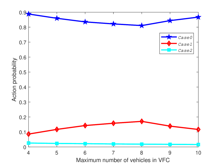
Fig. 3 shows the probabilities of , and for different maximum number of RUs in VFC when the task arrival rate is 20 and is 40 . We can see that the probability of always keeps a small value, which validates that our strategy can process most of tasks with high probability and only discard few tasks. In addition, the probability of is always larger than that of . This is because that the platoon has more available resources than VFC, and the system tends to offload the task to the platoon. Moreover, the probability of first gradually increases and the probability of first gradually decreases, because the resources in the VFC are gradually increasing with the increase of the maximum number of RUs in the VFC. In this case, more RUs in the VFC can be allocated to process tasks, which decreases the computing delay, thus the system tends to offload the tasks to the VFC to get a larger long-term reward. It also can be seen that the probability of is increasing while the probability of is decreasing as the maximum number of RUs continues to increase, because as the maximum number of RUs continues to increase, more vehicles in the VFC will face a higher collision probability and thus prolongs the transmitting delay. In this case, the system tends to offload the task to the platoon to get a higher long-term reward. In summary, there exists one best number of vehicles in VFC to deal with the tasks. This result will help us to control the number of VFC’s vehicles when designing VFC in applications.
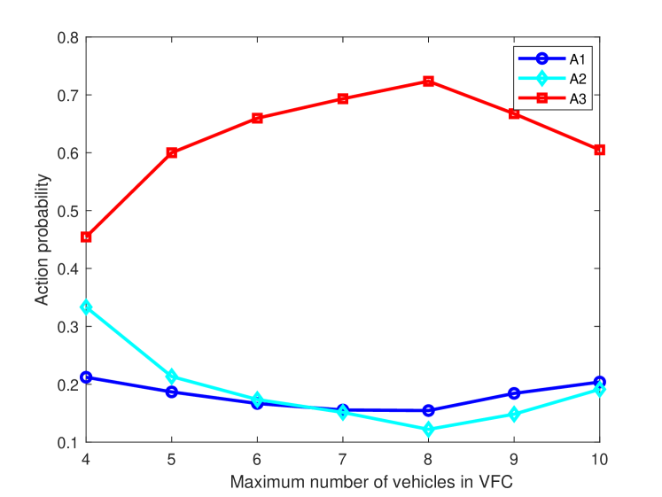
Fig. 4 shows the probabilities of , and when the task arrival rate is 20 and is 40 . We can see that the probability of is always larger than those of and , and the probability of is larger than that of at the beginning. This is because that the VFC needs to process a lot of tasks when the task arrival rate is 20 . The system tends to allocate RUs as many as possible to process the task, and the computing delay can be reduced. In addition, the probabilities of and first decrease and the probability of first increases with the increase of maximum number of RUs. This is because the resources in VFC gradually increase as the maximum number of RUs increases. The system tends to allocate more RUs in the VFC to reduce the computing delay and obtain a higher long-term reward. Moreover, the probability of becomes smaller than that of as the maximum number of RUs continues to increase. This is due to that the system allocates more RUs to process tasks due to the high probability of in the VFC, which increases the collision probability and transmitting delay. In this case, the system tends to allocate tasks to one RU rather than two RUs to reduce the collision probability. We can also observe that the probabilities of and increase and the probability of decreases as the maximum number of RUs continues to increase. This is because that more vehicles transmit data with the increase of the maximum number of RUs, which increases the collision probability and incurs a large transmitting delay. Thus the system will tend to allocate less RUs to process the task.
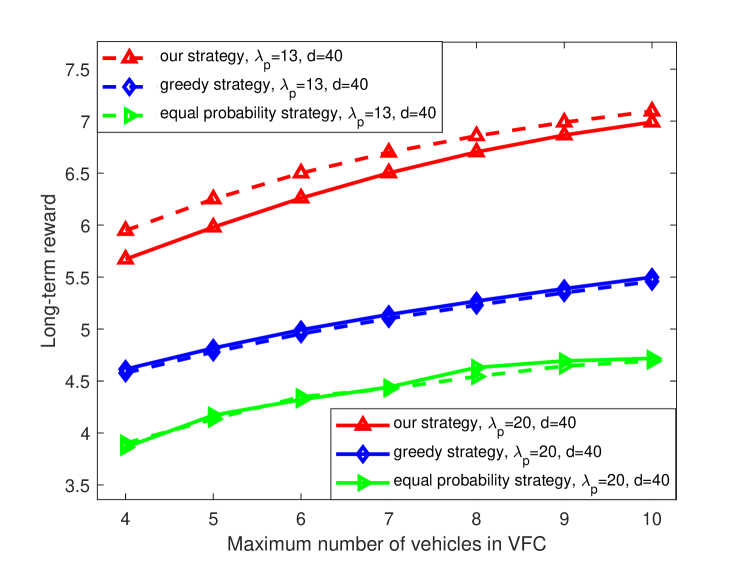
Fig. 5 shows the long-term rewards for different maximum numbers of vehicles in VFC, different strategies and task arrival rates when is 40 . We can see that the long-term reward of the system gradually under different strategies increases with the increase of the maximum number of vehicles in VFC. This is because that the available resource increases as the maximum number of vehicles in VFC increases, which reduces both computing delay and transmitting delay and further improves the long-term reward. In addition, we can find that under different task arrival rates, our proposed strategy can obtain a larger long-term reward than the greedy strategy while the equal probability strategy is inferior to greedy strategy. The reason is that the equal probability strategy does not consider the potential available resources in platoons and VFC, and the greedy strategy always allocates the maximum available resource in the system without considering the long-term reward, while our strategy jointly considers various factors to maximize the long-term reward. Moreover, we can see the long-term reward of our strategy for the task arrival rate being 20 is smaller than that for being 13 . This is because that when increases, there are more tasks in the system and thus the time of transmitting and processing tasks becomes longer, which results in smaller long-term reward. We also see that the long-term rewards of the greedy strategy and equal probability strategy are almost the same under different task arrival rates. This is because that the greedy strategy always allocates the maximum available resources for processing, and the equal probability strategy allocates resource based on equal probabilities without considering the variation of the task arrival rate.
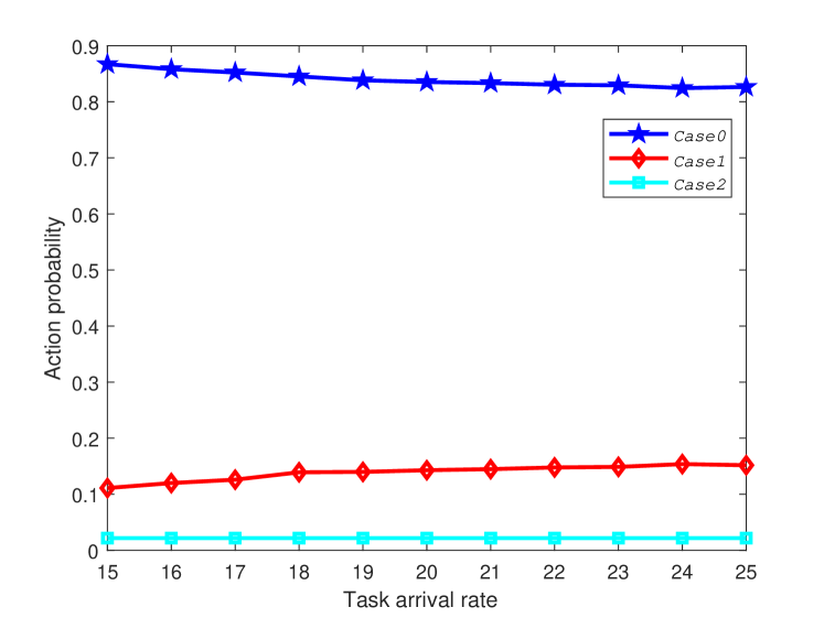
Fig. 6 shows the probabilities of , and for different task arrival rates when is 40 and is 6. We can see that our system can keep a small probability of discarding the tasks, which validates that our strategy can process most of tasks with high probability and only discard few tasks. In addition, the probability of is always larger than that of . This is because that the platoon has more available resources than VFC, and the system tends to offload the task to the platoon. When the task arrival rate is increasing, the probability of is decreasing and the probability of is increasing. This is because that the resources in the platoon are fixed, and thus when the task arriving rate is large, system tends to allocate more tasks to VFC to process quickly.
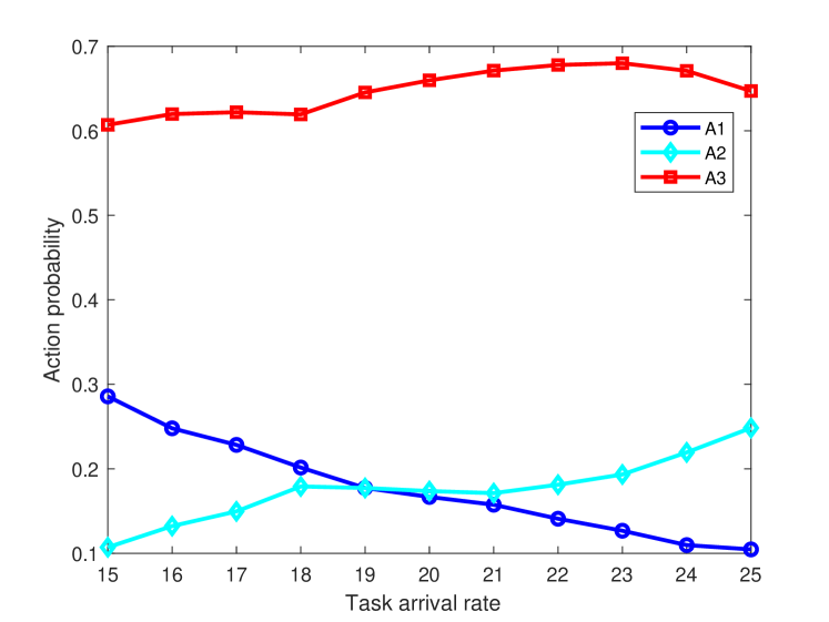
Fig. 7 shows the probabilities of , and for different task arrival rates when is 40 and is 6. We can see that when the task arrival rate increases, the probability of decreases, the probability of increases, and the probability of first increases and then decreases. This is becase that when the task arrival rate is small, the collision probability is small and allocating more RUs will lead to fast task processing. As the task arrival rate keeps increasing, allocating 3 RUs will lead a large collision probability because that each task will be divided to 3 subtasks to transmit. In this case, the negative impact caused by the collision probability will lead a large delay, which outweights the positive impact of fast task processing. Therefore, the probability of decreases when the task arrival rate is large.
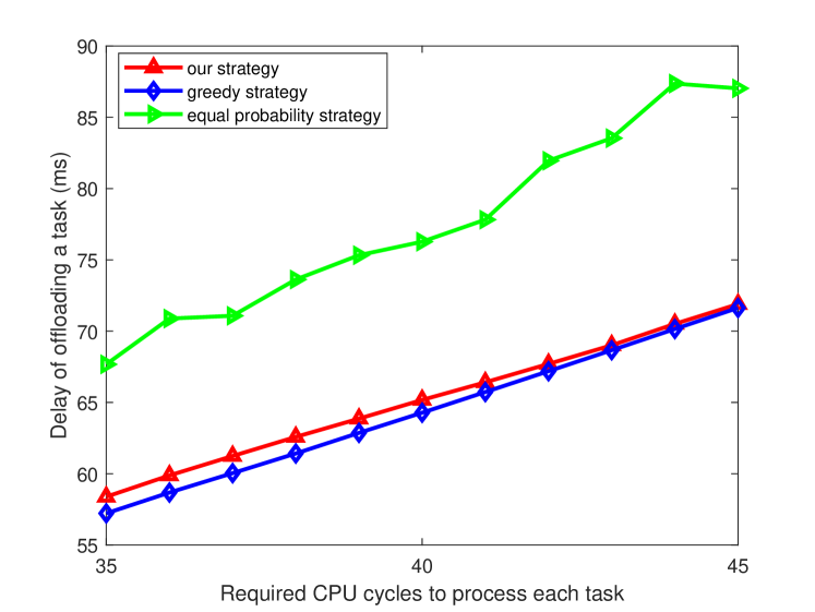
Fig. 8 shows the delay of offloading a task for different required CPU cycles to process each task and different strategies when is 20 and is 6. We can see that the offloading delay under different strategies increases with the increasing of required CPU cycles to process each task. This is the time of processing a task becoming longer, thus the offloading delay is also increased. We also see that the delay of the equal probability strategy is the highest and the delay of our strategy is slightly higher than that of the greedy strategy. This is because that the equal probability strategy allocates resource randomly without considering the performance including delay and resources consumption. In addition, our strategy has a slightly higher delay than that of the greedy strategy. This is because the optimization object of our strategy is not only the offloading delay but also the resource occupancy, which is detailed in Eq. (15). However, the system adopting greedy algorithm always chooses the available resource to minimize the offloading delay without considering the resource occupancy, thus its offloading delay is lower but its long-term reward is inferior to that of our strategy.
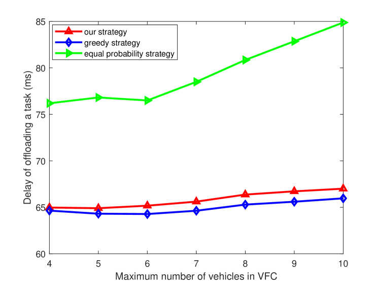
Fig. 9 shows the delay of offloading a task for different maximum numbers of vehicles and different strategies in VFC when is 20 and is 40 . We can see that the delay of different strategies increases with the maximum number of vehicles in VFC increases. It is because that with the number of vehicles in VFC increases, the collision probability increases, which causes more transmitting delay. Moreover, the delay of equal probability strategy is the highest and the delay of greedy algorithm is slightly lower than that of our strategy. This is due to the same reason as shown in Fig. 8.
VII Conclusions
In this paper, we jointly considered the 802.11p DCF mechanism, heterogeneous computation resource of vehicles in the platoon, random task arrival and departure as well as the random arrival and departure of vehicles in VFC. Then we proposed an offloading strategy to obtain the maximal long-term reward based on the SMDP. We first adopted the SMDP to model the offloading process and designed the SMDP framework including state set, action set, reward function and transition probability, where the transmitting delay are derived based on to the 802.11p DCF mechanism to determine the reward. Then we adopt the value iteration algorithm to solve the SMDP model to obtain the optimal offloading strategy. Extensive experiments have been conducted to demonstrate the outperformance of our strategy. According to the theoretical analysis and simulation results, the following conclusions are summarized:
-
•
Our strategy can process most of tasks and discard few tasks. In addition, the system prefers to offload to the platoon because the available resources in the platoon are larger than that in VFC. Moreover, there are more available RUs as the resources in the VFC increase, thus the system tends to offload task to the VFC. As the resources in the VFC keep increasing, the system tends to offload to the platoon due to the increase of the collision probability in the VFC.
-
•
The system under our strategy tends to allocate more RUs in the VFC for processing as increase of the resources in the VFC, but as the resources in the VFC keep increasing, the system tends to allocate less RUs for processing due to the increased collision probability in the platoon.
-
•
Our strategy performs better than the greedy strategy because the 802.11p DCF, heterogeneous computation resource of vehicles in the platoon, the random task arrival and departure as well as random arrival and departure of vehicles in VFC have been jointly considered to get the maximal long-term reward.
-
•
When the task is allocated to more RUs, the total delay which includes the transmitting delay in the platoon, transmitting delay form the leader vehicle to VFC and the computing delay in the RUs is small.
-
•
When and are fixed, different task arrival rates will influence the action probability of , , , , and . The offloading delay is increasing with the increase of required CPU cycles due to the increasing computing delay in the RUs.
Acknowledgment
The authors are indebted to Wenhua Wang and Jiahou Chu with Jiangnan University, for their help with this work.
References
- [1] Q. Wu, H. Ge, P. Fan, J. Wang, Q. Fan and Z. Li, “Time-Dependent Performance Analysis of the 802.11p-Based Platooning Communications Under Disturbance,” IEEE Transactions on Vehicular Technology, vol. 69, no. 12, pp. 15760-15773, 2020.
- [2] Q. Wu, S. Nie, P. Fan, H. Liu, Q. Fan and Z. Li, “A Swarming Approach to Optimize the One-Hop Delay in Smart Driving Inter-Platoon Communications,” Sensors, Vol. 18, No. 10, Doc. No. 3307, 2018.
- [3] N. Zhang, P. Yang, J. Ren, D. Chen, L. Yu and X. Shen, “Synergy of Big Data and 5G Wireless Networks: Opportunities, Approaches, and Challenges,” IEEE Wireless Communications, vol. 25, no. 1, pp. 12-18, 2018.
- [4] Jing Fan, Qiong Wu and Junfeng Hao, “Optimal Deployment of Wireless Mesh Sensor Networks based on Delaunay Triangulations,” in Proc. of IEEE International Conference on Information, Networking and Automation (ICINA’10), Kunming, China, Oct. 2010, pp. 1-5.
- [5] Q. Wu, Y. Zhao, Q. Fan, P. Fan, J. Wang and C. Zhang, “Mobility-Aware Cooperative Caching in Vehicular Edge Computing Based on Asynchronous Federated and Deep Reinforcement Learning,” IEEE Journal of Selected Topics in Signal Processing, vol. 17, no. 1, pp. 66-81, 2023.
- [6] Q. Wu, S. Shi, Z. Wan, Q. Fan, P. Fan and C. Zhang, “Towards V2I Age-aware Fairness Access: A DQN Based Intelligent Vehicular Node Training and Test Method,” Chinese Journal of Electronics, published online, 2022, doi: 10.23919/cje.2022.00.093.
- [7] X. Hou, Y. Li, M. Chen, D. Wu, D. Jin and S. Chen, “Vehicular Fog Computing: A Viewpoint of Vehicles as the Infrastructures,” IEEE Transactions on Vehicular Technology, vol. 65, no. 6, pp. 3860-3873, 2016.
- [8] X. Liu, W. Chen, Y. Xia and C. Yang, “SE-VFC: Secure and Efficient Outsourcing Computing in Vehicular Fog Computing,” IEEE Transactions on Network and Service Management, vol. 18, no. 3, pp. 3389-3399, 2021.
- [9] A. Hammoud, H. Otrok, A. Mourad and Z. Dziong, “On Demand Fog Federations for Horizontal Federated Learning in IoV,” IEEE Transactions on Network and Service Management, vol. 19, no. 3, pp. 3062-3075, 2022.
- [10] Z. Liu, Y. Yang, K. Wang, Z. Shao and J. Zhang, “POST: Parallel Offloading of Splittable Tasks in Heterogeneous Fog Networks,” IEEE Internet of Things Journal, vol. 7, no. 4, pp. 3170-3183, 2020.
- [11] N. Ding, S. Cui, C. Zhao, Y. Wang and B. Chen, “Multi-Link Scheduling Algorithm of LLC Protocol in Heterogeneous Vehicle Networks Based on Environment and Vehicle-Risk-Field Model,” IEEE Access, vol. 8, pp. 224211-224223, 2020.
- [12] Qiong Wu and Jun Zheng, “Performance Modeling of the IEEE 802.11p EDCA Mechanism for VANET,” in Proc. of IEEE Global Communications Conference (Globecom’14), Austin, USA, Dec. 2014, pp. 57-63.
- [13] Q. Wu, S. Xia, P. Fan, Q. Fan and Z. Li, “Velocity-Adaptive V2I Fair Access Scheme Based on IEEE 802.11 DCF for Platooning Vehicles,” Sensors, No. 4198, Dec. 2018.
- [14] H. Nguyen, X. Xiaoli, Md. Noor-A-Rahim, Y. Guan, D. Pesch, H. Li and A. Filippi. “Impact of Big Vehicle Shadowing on Vehicle-to-Vehicle Communications,” IEEE Transactions on Vehicular Technology, vol. 69, no. 7, pp. 6902-6915, 2020.
- [15] J. Zheng, Q. Wu, “Performance Modeling and Analysis of the IEEE 802.11p EDCA Mechanism for VANET,” IEEE Transactions on Vehicular Technology, Vol. 65, No. 4, pp. 2673-2687, 2016.
- [16] X. Fan, T. Cui, C. Cao, Q. Chen and K. Kwak. “Minimum-Cost Offloading for Collaborative Task Execution of MEC-Assisted Platooning,” Sensors, vol. 19, no. 4, pp. 847, 2019.
- [17] X. Ma, J. Zhao, Q. Li and Y. Gong. “Reinforcement learning based task offloading and take-back in vehicle platoon networks,” 2019 IEEE International Conference on Communications Workshops (ICC Workshops), Shanghai, China, 2019, pp. 1-6, doi: 10.1109/ICCW.2019.8756836.
- [18] Y. Hu, T. Cui, X. Huang and Q.Chen. “Task Offloading Based on Lyapunov Optimization for MEC-assisted Platooning,” 2019 11th International Conference on Wireless Communications and Signal Processing (WCSP), Xi’an, China, 2019, pp. 1-5, doi: 10.1109/WCSP.2019.8928035.
- [19] H. Du, S. Leng, F. Wu and L. Zhou, “A Communication Scheme for Delay Sensitive Perception Tasks of Autonomous Vehicles,” 2020 IEEE 20th International Conference on Communication Technology (ICCT), Nanning, China, 2020, pp. 687-691, doi: 10.1109/ICCT50939.2020.9295766.
- [20] D. Zheng, Y. Chen, L. Wei, B.Jiao and L. Hanzo. “Dynamic NOMA-Based Computation Offloading in Vehicular Platoons,” IEEE Transactions on Vehicular Technology, doi: 10.1109/TVT.2023.3274252.
- [21] T. Xiao, C. Chen, Q. Pei and H. H. Song, “Consortium Blockchain-Based Computation Offloading Using Mobile Edge Platoon Cloud in Internet of Vehicles,” IEEE Transactions on Intelligent Transportation Systems, vol. 23, no. 10, pp. 17769-17783, Oct. 2022, doi: 10.1109/TITS.2022.3168358.
- [22] H. Liao, Z. Zhou, X. Zhao, B. Ai and S. Mumtaz, “Task Offloading for Vehicular Fog Computing under Information Uncertainty: A Matching-Learning Approach,” 2019 15th International Wireless Communications and Mobile Computing Conference (IWCMC), Tangier, Morocco, 2019, pp. 2001-2006, doi: 10.1109/IWCMC.2019.8766579.
- [23] Z. Zhou, H. Liao, X. Wang, S. Mumtaz and J. Rodriguez, “When Vehicular Fog Computing Meets Autonomous Driving: Computational Resource Management and Task Offloading,” IEEE Network, vol. 34, no. 6, pp. 70-76, 2020.
- [24] J. Shi, J. Du, J. Wang, J. Wang and J. Yuan, “Priority-Aware Task Offloading in Vehicular Fog Computing Based on Deep Reinforcement Learning,” IEEE Transactions on Vehicular Technology, vol. 69, no. 12, pp. 16067-16081, 2020.
- [25] R. Yadav, W. Zhang, O. Kaiwartya, H. Song and S. Yu, “Energy-Latency Tradeoff for Dynamic Computation Offloading in Vehicular Fog Computing,” IEEE Transactions on Vehicular Technology, vol. 69, no. 12, pp. 14198-14211, 2020.
- [26] J. Xie, Y. Jia, Z. Chen, Z. Nan and L. Liang, “Efficient task completion for parallel offloading in vehicular fog computing,” China Communications, vol. 16, no. 11, pp. 42-55, 2019.
- [27] S. Iqbal, A. W. Malik, A. U. Rahman and R. M. Noor, “Blockchain-Based Reputation Management for Task Offloading in Micro-Level Vehicular Fog Network,” IEEE Access, vol. 8, pp. 52968-52980, 2020, doi: 10.1109/ACCESS.2020.2979248.
- [28] S. Misra and S. Bera, “Soft-VAN: Mobility-Aware Task Offloading in Software-Defined Vehicular Network,” IEEE Transactions on Vehicular Technology, vol. 69, no. 2, pp. 2071-2078, 2020.
- [29] C. Liu, K. Liu, X. Xu, H. Ren, F. Jin and S. Guo, “Real-time Task Offloading for Data and Computation Intensive Services in Vehicular Fog Computing Environments,” 2020 16th International Conference on Mobility, Sensing and Networking (MSN), Tokyo, Japan, 2020, pp. 360-366, doi: 10.1109/MSN50589.2020.00066.
- [30] K. Wang, Y. Tan, Z. Shao, S. Ci and Y. Yang, “Learning-Based Task Offloading for Delay-Sensitive Applications in Dynamic Fog Networks,” IEEE Transactions on Vehicular Technology, vol. 68, no. 11, pp. 11399-11403, 2019.
- [31] C. Zhu, J. Tao, G. Pastor, Y. Xiao, Y. Ji, Q. Zhou, Y. Li and A. Ylä-Jääski. “Folo: Latency and Quality Optimized Task Allocation in Vehicular Fog Computing,” IEEE Internet of Things Journal, vol. 6, no. 3, pp. 4150-4161, 2019.
- [32] J. Zhao, M. Kong, Q. Li and X. Sun, “Contract-Based Computing Resource Management via Deep Reinforcement Learning in Vehicular Fog Computing,” IEEE Access, vol. 8, pp. 3319-3329, 2020, doi: 10.1109/ACCESS.2019.2963051.
- [33] W. Tang, S. Li, W. Rafique, W. Dou and S. Yu, “An Offloading Approach in Fog Computing Environment,” 2018 IEEE SmartWorld, Ubiquitous Intelligence and Computing, Advanced and Trusted Computing, Scalable Computing and Communications, Cloud and Big Data Computing, Internet of People and Smart City Innovation (SmartWorld/SCALCOM/UIC/ATC/CBDCom/IOP/SCI), Guangzhou, China, 2018, pp. 857-864, doi: 10.1109/SmartWorld.2018.00157.
- [34] B. Yang, M. Sun, X. Hong and X. Guo, “A Deadline-Aware Offloading Scheme for Vehicular Fog Computing at Signalized Intersection,” 2020 IEEE International Conference on Pervasive Computing and Communications Workshops (PerCom Workshops), Austin, TX, USA, 2020, pp. 1-6, doi: 10.1109/PerComWorkshops48775.2020.9156078.
- [35] A. Mourad, H. Tout, O. A. Wahab, H. Otrok and T. Dbouk, “Ad Hoc Vehicular Fog Enabling Cooperative Low-Latency Intrusion Detection,” IEEE Internet of Things Journal, vol. 8, no. 2, pp. 829-843, 2021.
- [36] C. Liu, K. Liu, S. Guo, R. Xie, V. C. S. Lee and S. H. Son, “Adaptive Offloading for Time-Critical Tasks in Heterogeneous Internet of Vehicles,” IEEE Internet of Things Journal, vol. 7, no. 9, pp. 7999-8011, 2020.
- [37] B. Cho and Y. Xiao, “Learning-Based Decentralized Offloading Decision Making in an Adversarial Environment,” IEEE Transactions on Vehicular Technology, vol. 70, no. 11, pp. 11308-11323, 2021.
- [38] Y. Wu, J. Wu, L. Chen, G. Zhou and J. Yan, “Fog Computing Model and Efficient Algorithms for Directional Vehicle Mobility in Vehicular Network,” IEEE Transactions on Intelligent Transportation Systems, vol. 22, no. 5, pp. 2599-2614, 2021.
- [39] X. Huang, L. He, X. Chen, L. Wang and F. Li, “Revenue and Energy Efficiency-Driven Delay-Constrained Computing Task Offloading and Resource Allocation in a Vehicular Edge Computing Network: A Deep Reinforcement Learning Approach,” IEEE Internet of Things Journal, vol. 9, no. 11, pp. 8852-8868, 2022.
- [40] M. Z. Alam and A. Jamalipour, “Multi-Agent DRL-based Hungarian Algorithm (MADRLHA) for Task Offloading in Multi-Access Edge Computing Internet of Vehicles (IoVs),” IEEE Transactions on Wireless Communications, vol. 21, no. 9, pp. 7641-7652, 2022.
- [41] W. Fan, J. Liu, M. Hua, F. Wu and Y. Liu, “Joint Task Offloading and Resource Allocation for Multi-Access Edge Computing Assisted by Parked and Moving Vehicles,” IEEE Transactions on Vehicular Technology, vol. 71, no. 5, pp. 5314-5330, 2022.
- [42] Y. Chen, F. Zhao, X. Chen and Y. Wu, “Efficient Multi-Vehicle Task Offloading for Mobile Edge Computing in 6G Networks,” IEEE Transactions on Vehicular Technology, vol. 71, no. 5, pp. 4584-4595, 2022.
- [43] C. Chen, Y. Zeng, H. Li, Y. Liu and S. Wan, “A Multi-hop Task Offloading Decision Model in MEC-enabled Internet of Vehicles,” IEEE Internet of Things Journal, vol. 10, no. 4, pp. 3215-3230, 2023.
- [44] Y. Lin, Y. Zhang, J. Li, F. Shu and C. Li, “Popularity-Aware Online Task Offloading for Heterogeneous Vehicular Edge Computing Using Contextual Clustering of Bandits,” IEEE Internet of Things Journal, vol. 9, no. 7, pp. 5422-5433, 2022.
- [45] L. Liu, M. Zhao, M. Yu, M. A. Jan, D. Lan and A. Taherkordi, “Mobility-Aware Multi-Hop Task Offloading for Autonomous Driving in Vehicular Edge Computing and Networks,” IEEE Transactions on Intelligent Transportation Systems, vol. 24, no. 2, pp. 2169-2182, 2023.
- [46] B. Ma, Z. Ren and W. Cheng, “Traffic Routing-Based Computation Offloading in Cybertwin-Driven Internet of Vehicles for V2X Applications,” IEEE Transactions on Vehicular Technology, vol. 71, no. 5, pp. 4551-4560, 2022.
- [47] K. Zheng, H. Meng, P. Chatzimisios, L. Lei and X. Shen, “An SMDP-Based Resource Allocation in Vehicular Cloud Computing Systems,” IEEE Transactions on Industrial Electronics, vol. 62, no. 12, pp. 7920-7928, 2015.
- [48] C. Wang, C. Liang, F. R. Yu, Q. Chen and L. Tang, “Computation Offloading and Resource Allocation in Wireless Cellular Networks With Mobile Edge Computing,” IEEE Transactions on Wireless Communications, vol. 16, no. 8, pp. 4924-4938, 2017.
- [49] Wireless LAN Medium Access Control (MAC) and Physical Layer (PHY) Specifications Amendment 7: Wireless Access in Vehicular Environments, IEEE Std. P802.11p/D8.0, Jul. 2009.
- [50] D. Malone, K. Duffy and D. Leith, “Modeling the 802.11 Distributed Coordination Function in Nonsaturated Heterogeneous Conditions,” IEEE/ACM Transactions on Networking, vol. 15, no. 1, pp. 159-172, 2007.
- [51] Q. Wu, H. Liu, C. Zhang, Q. Fan, Z. Li and K. Wang, “Trajectory Protection Schemes Based on a Gravity Mobility Model in IoT,” Electronics, Vol. 8, No. 148, 2019.
- [52] Q. Wu, J. Zheng, “Performance Modeling and Analysis of the ADHOC MAC Protocol for Vehicular Networks,” Wireless Networks, Vol. 22, No. 3, pp. 799-812, 2016.
- [53] G. Bianchi, “Performance analysis of the IEEE 802.11 distributed coordination function,” IEEE Journal on Selected Areas in Communications, vol. 18, no. 3, pp. 535-547, 2000.
- [54] Q. Wu, H. Liu, R. Wang, P. Fan, Q. Fan and Z. Li, “Delay Sensitive Task Offloading in the 802.11p Based Vehicular Fog Computing Systems,” IEEE IoT-J, vol. 7, no. 1, pp. 773-785, 2020.
- [55] S. Mine and M. Puterman, “Markovian Decision Process,” Amsterdam, The Netherlands: Elsevier, 1970.
- [56] M. Puterman, “Markov Decision Processes: Discrete Stochastic Dynamic Programming,” New York, NY , USA: Wiley, 2005.
- [57] B. Luo, Y. Yang, H. -N. Wu and T. Huang, “Balancing Value Iteration and Policy Iteration for Discrete-Time Control,” IEEE Transactions on Systems, Man, and Cybernetics: Systems, vol. 50, no. 11, pp. 3948-3958, 2020.
- [58] M. Puterman, Markov Decision Processes: Discrete Stochastic Dynamic Programming, New York, NY, USA: Wiley, 2005.
- [59] T. Cormen, C. Leiserson, R. Rivest and C. Stein, Introduction to Algorithms, Cambridge, MA, USA: MIT Press, 2001.