Delicatessen: M-Estimation in Python
2Institute of Global Health and Infectious Diseases, School of Medicine, University of North Carolina at Chapel Hill, Chapel Hill, NC
3Department of Biostatistics, Gillings School of Global Public Health, University of North Carolina at Chapel Hill, Chapel Hill, NC
September 27, 2025)
Abstract
M-estimation is a general statistical framework that simplifies estimation. Here, we introduce delicatessen, a Python library that automates the tedious calculations of M-estimation, and supports both built-in user-specified estimating equations. To highlight the utility of delicatessen for quantitative data analysis, we provide several illustrations common to life science research: linear regression robust to outliers, estimation of a dose-response curve, and standardization of results.
M-estimation is a general large-sample statistical framework [1]. Widespread application of M-estimation is hindered by tedious derivative and matrix calculations. To address this barrier, we developed delicatessen, an open-source Python library that flexibly automates the mathematics of M-estimation. Delicatessen supports both built-in and custom, user-specified estimating equations. To help contextualize the value of M-estimation and delicatessen, we showcase several applications common to statistical analyses in life sciences research: regression with outliers, dose-response curves, and standardization.
To begin, we briefly review M-estimation; see Stefanski and Boos (2002) for a thorough introduction [1]. An M-estimator, , is the solution for to the vector equation , where is the parameter vector, is a ()-dimension estimating equation, and are the observed data for independent and identically distributed units. As an example, the M-estimator for the mean () of a variable () is , which is equivalent to the usual mean estimator, . To find , root-finding procedures can be used, which iteratively search for the value(s) of where . The variance of can be estimated using the empirical sandwich variance estimator (see Appendix). Key advantages of the sandwich estimator are reduced computational burden for variance estimation relative to common alternatives (e.g., bootstrapping [2, 3], Monte Carlo methods [4], etc.), automation of the delta method, and valid variance estimation for parameters that depend on other estimated parameters [1].
M-estimators are implemented in delicatessen via the MEstimator class. Input to MEstimator includes the estimating equation(s) and starting values for the root-finding algorithm. Root-finding algorithms implemented in SciPy [5], as well as custom root-finding algorithms, are supported. After finding , the ‘bread’ of the sandwich estimator is calculated by numerically approximating the partial derivatives via the central difference formula and the ‘filling’ of the sandwich is calculated using NumPy [6]. Finally, the sandwich covariance matrix is constructed. While other M-estimation implementations exist [7, 8, 9], delicatessen provides greater support for both user-specified and pre-built estimating equations (Appendix Table 1).
To demonstrate application of delicatessen, we provide three examples common to life sciences research. First, consider linear regression with outliers [10, 11]. A common approach to handling outliers is to exclude them. However, exclusion ignores all information contributed by outliers, and should only be done when outliers are unambiguously a result of experimental error [11]. Yet, including outliers with simple linear regression can lead to unstable or unreliable estimates. Robust regression has been proposed as an alternative, whereby outliers contribute but their influence is curtailed [12, 13]. The estimating equations for the intercept and slope with robust linear regression are
where is the independent variable, is the dependent variable(s), is the parameter vector for the regression model, and truncates or bounds the residuals at . To illustrate, 15 observations were simulated following Altman & Krzywinski (2016) [11] and all models were fit using delicatessen with built-in estimating equations. As a reference, a linear model was fit to the simulated data (Figure 1a, original reference slope: ). An outlying value of was then generated by replacing with for the observation with the smallest value. When fitting a linear model with this outlier, the slope is noticeably decreased (). With robust regression and [14], the influence of the outlier was curtailed and the estimated slope () was closer to the reference.
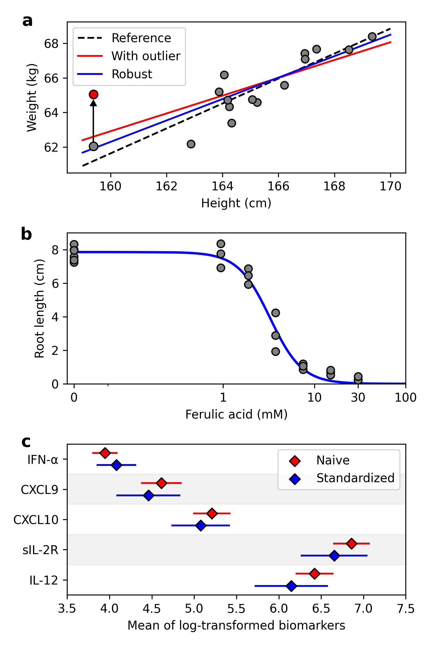
a: The reference line was estimated using simple linear regression based on the gray data points. The ‘with outlier’ simple and ‘robust’ were estimated with the induced outlier, indicated by the red data point.
b: Dose-response curve for herbicide on ryegrass root length. Dots indicate the data points, and the blue line is the estimated dose-response curve.
c: Forest plot for the mean of the log-transformed biomarkers. Naive corresponds to the means for the original HIV patients. Standardized corresponds to the inverse odds weighted means. Lines indicate the 95% confidence intervals.
As the second example, consider estimating the dose-response curve of herbicides on ryegrass root length [15, 16]. Since there is a natural lower bound of zero on root length, a three-parameter log-logistic (3PL) model was used. Parameters of the 3PL model are the halfway maximum effective concentration (), steepness of the dose-response curve (), and upper limit on the response (). Let denote the estimating equations (see Appendix), where is the dose and is the response. Besides the halfway maximum effective concentration, other concentration levels may also be of interest. Let denote the % effective concentration, where . Here, estimation of the 20% effective concentration was of interest, with the estimating equation . As is a transformation of the other parameters, this estimating equation does not depend on the observations but is instead a delta-method transformation of the parameters. Here, the estimating equations can be ‘stacked’ together
where . The variance for is automatically estimated through the sandwich. The sandwich variance can then be used to construct Wald-type 95% confidence intervals (CI). The estimated dose-response curve using delicatessen and the built-in estimating equations is shown in Figure 1b. The estimated 20% effective concentration was 1.86 (95% CI: 1.58, 2.14). This example highlights how M-estimation can be used to apply the delta method, with delicatessen automating the process.
Finally, consider the problem of standardization. Often the available data is not a random sample of the population. Consider the biomarker data from a convenience sample of HIV patients () in Kamat et al. (2012) [17]. When comparing the prevalence of recent drug use (either cocaine or opiates) to a more generalizable cohort,[18] drug use was notably higher in Kamat et al.’s sample (70% versus 8%). As Kamat et al. reported differential biomarker expression by cocaine use, differential patterns in drug use between data sets indicates that the summary statistics on biomarker expression may not be generalizable. To account for the discrepancy in drug use, we standardized the mean for select biomarkers to the distribution of drug use in the secondary data source using inverse odds weights [19]. Inverse odds weights were estimated using a logistic regression model [20], with the estimating equations
where indicates drug use for individual , indicates if the individual was in the Kamat et al. study () or in the cohort (), and is the inverse logit. The estimating equation for the weighted mean is
where is the log-transformed biomarker , is the mean for biomarker , and
is the inverse odds weight. While is not of primary interest, the estimates of depend on through the inverse odds weights. This dependence means that the estimated variance of should carry forward into the estimated variance of . Ignoring this dependence puts us in danger of underestimating the uncertainty in the means for biomarker expression. M-estimators address this issue via the sandwich, where the uncertainty of parameters are propagated through the stacked estimating equations. Therefore, estimating equations for the logistic model and for the biomarker means were stacked together and . The stacked estimating equations were implemented in delicatessen by a combination of built-in and user-specified estimating equations. Results for select biomarkers are presented in Figure 1c. Notably, the means for log-transformed sIL-2R and IL-12 decreased after standardization. While these results were standardized by drug use, definitions varied between studies and other important differences between the populations the samples were drawn from likely exist. Therefore, these results should only be viewed as an illustration of how M-estimation can be used.
To summarize, M-estimation is a flexible framework. To automate the mathematics of M-estimators, we developed delicatessen, which supports both pre-built and user-created estimating equations. Key features of delicatessen were highlighted through examples in life science research. Further examples can be found on our website.
Acknowledgments
The authors would like to thank Drs. Michael Love, Adaora Adimora, and trainees on HIV/STI training grant at University of North Carolina at Chapel Hill for their feedback.
PNZ was supported by T32-AI007001 at the time of the software development and writing of this paper.
All code is available on GitHub (github.com/pzivich/Delicatessen) and through the Python Package Index. Documentation and further examples can be found on GitHub and the project website (deli.readthedocs.io/en/latest/). Feature requests, bug reports, or help requests can be done through the GitHub repository.
References
- [1] L. A. Stefanski and D. D. Boos, “The calculus of m-estimation,” The American Statistician, vol. 56, no. 1, pp. 29–38, 2002.
- [2] B. Efron, “Nonparametric estimates of standard error: the jackknife, the bootstrap and other methods,” Biometrika, vol. 68, no. 3, pp. 589–599, 1981.
- [3] A. Kulesa, M. Krzywinski, P. Blainey, and N. Altman, “Sampling distributions and the bootstrap,” Nature Methods, vol. 12, pp. 477–478, 2015.
- [4] G. Hamra, R. MacLehose, and D. Richardson, “Markov chain monte carlo: an introduction for epidemiologists,” International journal of epidemiology, vol. 42, no. 2, pp. 627–634, 2013.
- [5] P. Virtanen, R. Gommers, T. E. Oliphant, M. Haberland, T. Reddy, D. Cournapeau, E. Burovski, P. Peterson, W. Weckesser, J. Bright, et al., “Scipy 1.0: fundamental algorithms for scientific computing in python,” Nature Methods, vol. 17, no. 3, pp. 261–272, 2020.
- [6] C. R. Harris, K. J. Millman, S. J. Van Der Walt, R. Gommers, P. Virtanen, D. Cournapeau, E. Wieser, J. Taylor, S. Berg, N. J. Smith, et al., “Array programming with numpy,” Nature, vol. 585, no. 7825, pp. 357–362, 2020.
- [7] B. C. Saul and M. G. Hudgens, “The calculus of m-estimation in r with geex,” Journal of Statistical Software, vol. 92, no. 2, 2020.
- [8] F. Pedregosa, G. Varoquaux, A. Gramfort, V. Michel, B. Thirion, O. Grisel, M. Blondel, P. Prettenhofer, R. Weiss, V. Dubourg, et al., “Scikit-learn: Machine learning in python,” the Journal of Machine Learning Research, vol. 12, pp. 2825–2830, 2011.
- [9] S. Seabold and J. Perktold, “Statsmodels: Econometric and statistical modeling with python,” in Proceedings of the 9th Python in Science Conference, vol. 57, p. 61, Austin, TX, 2010.
- [10] N. Altman and M. Krzywinski, “Points of significance: Simple linear regression.,” Nature Methods, vol. 12, no. 11, 2015.
- [11] N. Altman and M. Krzywinski, “Analyzing outliers: influential or nuisance?,” Nature Methods, vol. 13, no. 4, pp. 281–283, 2016.
- [12] P. J. Huber, “Robust estimation of a location parameter,” in Breakthroughs in Statistics, pp. 492–518, Springer, 1992.
- [13] P. J. Huber, “Robust regression: asymptotics, conjectures and monte carlo,” The Annals of Statistics, pp. 799–821, 1973.
- [14] P. J. Huber, Robust statistics, vol. 523. John Wiley & Sons, 2004.
- [15] Inderjit, J. C. Streibig, and M. Olofsdotter, “Joint action of phenolic acid mixtures and its significance in allelopathy research,” Physiologia Plantarum, vol. 114, no. 3, pp. 422–428, 2002.
- [16] C. Ritz, F. Baty, J. C. Streibig, and D. Gerhard, “Dose-response analysis using r,” PloS One, vol. 10, no. 12, p. e0146021, 2015.
- [17] A. Kamat, V. Misra, E. Cassol, P. Ancuta, Z. Yan, C. Li, S. Morgello, and D. Gabuzda, “A plasma biomarker signature of immune activation in hiv patients on antiretroviral therapy,” PloS one, vol. 7, no. 2, p. e30881, 2012.
- [18] G. D’Souza, F. Bhondoekhan, L. Benning, J. B. Margolick, A. A. Adedimeji, A. A. Adimora, M. L. Alcaide, M. H. Cohen, R. Detels, M. R. Friedman, et al., “Characteristics of the macs/wihs combined cohort study: opportunities for research on aging with hiv in the longest us observational study of hiv,” American journal of epidemiology, vol. 190, no. 8, pp. 1457–1475, 2021.
- [19] D. Westreich, J. K. Edwards, C. R. Lesko, E. Stuart, and S. R. Cole, “Transportability of trial results using inverse odds of sampling weights,” American journal of epidemiology, vol. 186, no. 8, pp. 1010–1014, 2017.
- [20] J. Lever, M. Krzywinski, and N. Altman, “Logistic regression: Regression can be used on categorical responses to estimate probabilities and to classify,” Nature Methods, vol. 13, no. 7, pp. 541–543, 2016.
Appendix
Empirical Sandwich Covariance Estimator
The empirical sandwich variance estimator, , for the asymptotic covariance matrix is
where the ‘bread’ of the sandwich estimator is
with indicating the matrix derivative, and the ‘filling’ of the sandwich estimator is
The finite sample variance estimator is obtained by scaling the asymptotic variance estimate by , .
Estimating Equations
The estimating equations for the 3-parameter log-logistic model with a lower dose-response limit of zero are
where and . The first, second, and third estimating equations are for , , and , respectively. The effective dose estimating equation is
As previously stated, the effective dose estimating equation is a transformation of the 3-parameter log-logistic model parameters (i.e., it does not depend on or ).
| Built-in EE | |||||||||||||||
| Library | Language |
|
|
|
|
g-computation | IPW | AIPW | |||||||
| delicatessen | Python | x | x | x | x | x | x | x | |||||||
| statsmodels | Python | x | x | ||||||||||||
| sklearn | Python | x | |||||||||||||
| geex | R | x | |||||||||||||
| sandwich | R | x | x | ||||||||||||
| MASS | R | x | x | ||||||||||||
| rlm | R | x | |||||||||||||
| drc | R | x | |||||||||||||
| Mestimation | Julia | x | |||||||||||||
EE: estimating equation(s). IPW: inverse probability weighting, AIPW: augmented inverse probability weighting.
* Available features based on most recent version of each software as of 2022/02/13.
See pages - of appendix_code.pdf