Demonstration of an optical-coherence converter

In general $S\leq S_{\mathrm{p}}+S_{\mathrm{s}}$, with equality achieved only when the two DoFs are independent, in which case $\mathbf{G}$ can be written in separable form $\mathbf{G}=\mathbf{G}_{\mathrm{s}}\otimes\mathbf{G}_{\mathrm{p}}$. In general, $S_{\mathrm{s}}$ and $S_{\mathrm{p}}$ are obtained from the $2\times 2$ ‘reduced’ spatial and polarization coherency matrices

which are obtained from $\mathbf{G}$ by a ‘partial trace’ ¹⁹, that is, by tracing over one DoF ^{6; 7}

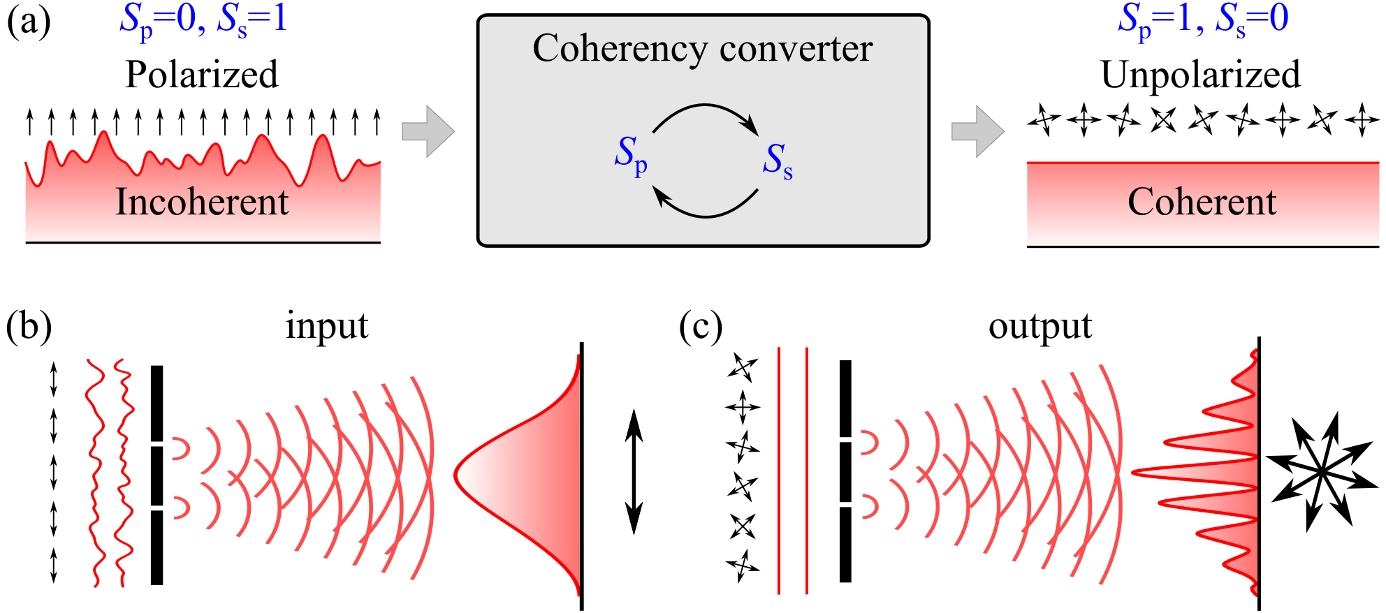
The concept of an optical-coherence converter is illustrated in Fig. 1(a). Consider the case when the field carries one bit of entropy ($S=1$) and the DoFs are independent ($S=S_{\mathrm{p}}+S_{\mathrm{s}}$), in which case a single DoF can accommodate this entropy. The field may be maximally incoherent but polarized ($S_{\mathrm{s}}=1$ and $S_{\mathrm{p}}=0$), whereupon no interference fringes can be observed [Fig. 1(b)]. Alternatively, the field may be spatially coherent but unpolarized ($S_{\mathrm{s}}=0$ and $S_{\mathrm{p}}=1$), in which case full-visibility fringes can be observed [Fig. 1(c)]. We demonstrate here that an optical field can be reversibly transformed from the former configuration to the latter without loss of energy, thus converting coherence from one DoF (polarization) to the other (spatial). Throughout the procedure $S$ remains constant; that is, no uncertainty is added or removed from the field, only an internal reorganization of the field engendered by a unitary transformation confines the statistical fluctuations to one DoF while freeing the other from uncertainty. We call such a system a ‘coherence converter’.

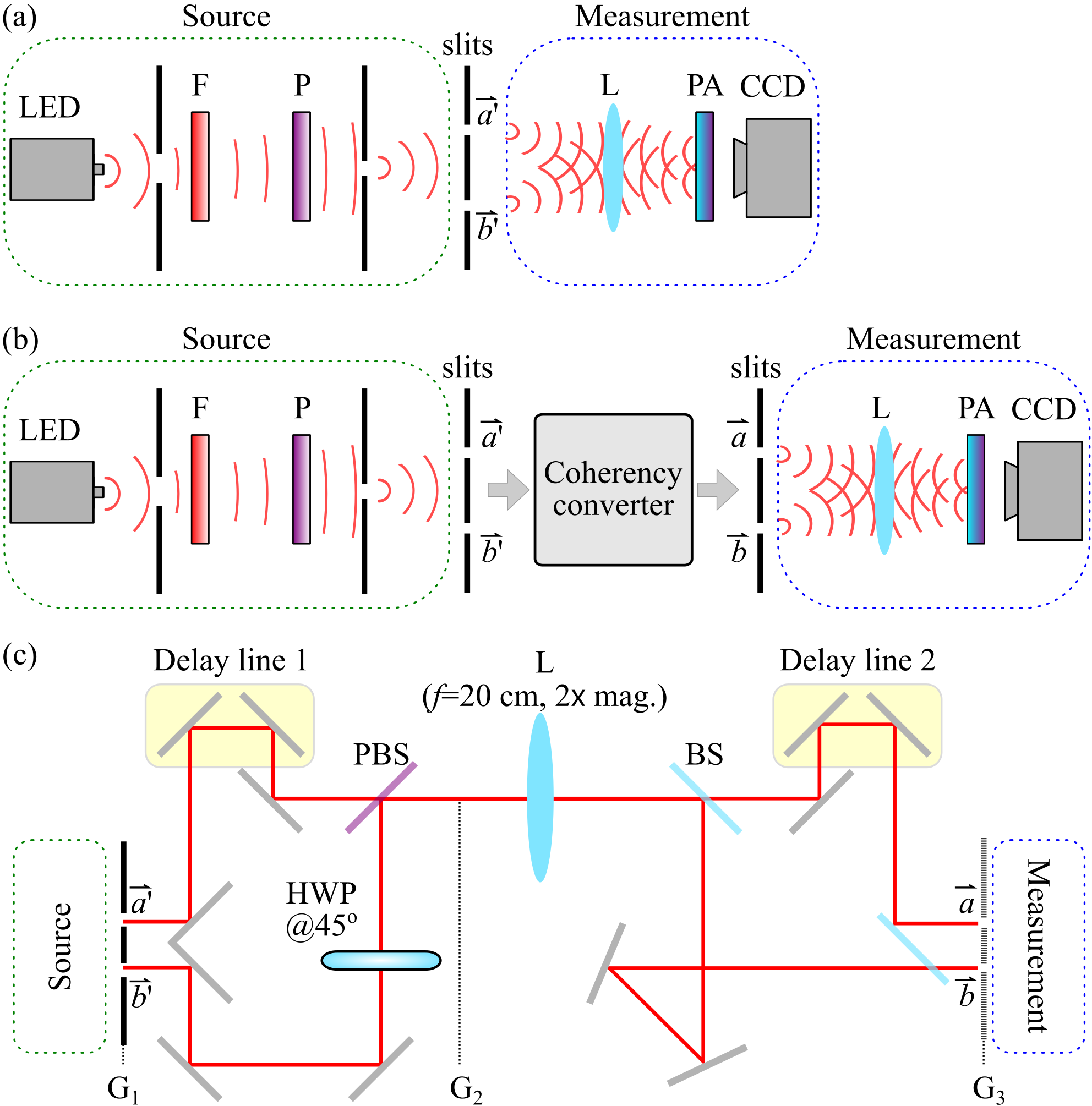
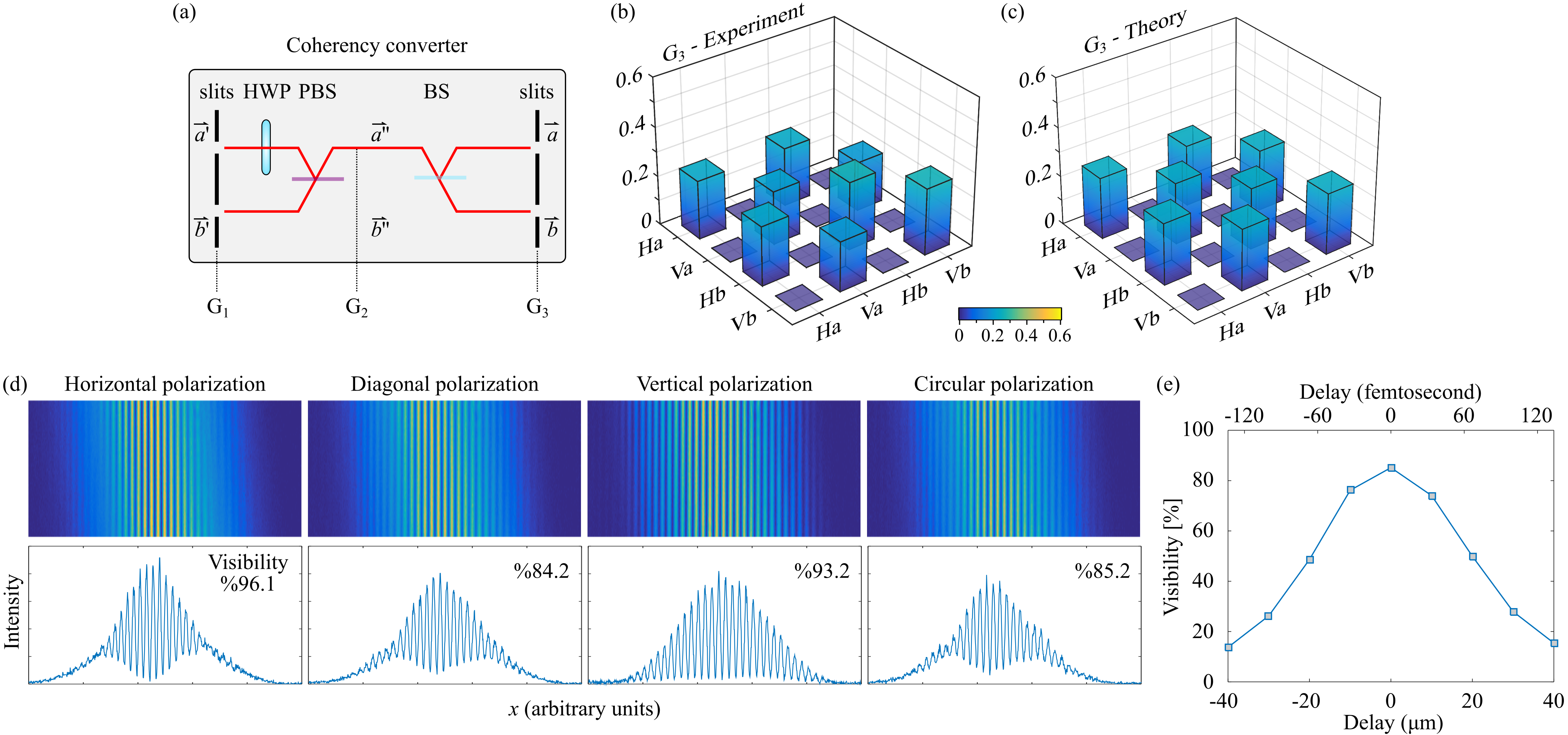
The optical arrangement we propose to convert coherency between the spatial and polarization DoFs is depicted in Fig. 2. We start from two points $\vec{a}^{\prime}$ and $\vec{b}^{\prime}$ of equal intensity in a spatially incoherent H-polarized field (the fields are mutually incoherent or statistically independent), which thus produce no interference fringes. The polarization at $\vec{b}^{\prime}$ is rotated to become orthogonal to that at $\vec{a}^{\prime}$ $(\mathrm{H}\rightarrow\mathrm{V})$ before combining the fields at a polarizing beam splitter (PBS), which yields an unpolarized field. We then split the field into two points $\vec{a}$ and $\vec{b}$ using a nonpolarizing beam splitter, which creates two copies of the field that can demonstrate high-visibility interference fringes. We proceed now to present the measurements at each step of this coherency-conversion process.

The optical field we study is extracted from a broadband, unpolarized LED (center wavelength 850 nm, 30-nm-FWHM bandwidth; Thorlabs M850L3 IR). The field is spectrally filtered (10-nm-FWHM), polarized along H, and spatially filtered through a 100-$\mu$m-wide slit placed at a distance of 180 mm from the source. The ‘input’ plane that includes the points $\vec{a}^{\prime}$ and $\vec{b}^{\prime}$ (each defined by a 100-$\mu$m-wide slit) is located 420 mm away from the slit [the source in Fig. 2(a)]. We first confirm that the field is spatially coherent within $\vec{a}^{\prime}$ and $\vec{b}^{\prime}$ separately (i.e., the spatial coherence width of the field, estimated to be $\sim$1 mm, is larger than the slit width). This is accomplished using a narrow pair of slits (50-$\mu$m-wide separated by $\Delta=150$ $\mu$m) at either $\vec{a}^{\prime}$ or $\vec{b}^{\prime}$ and observing the double-slit interference on a CCD camera (Hamamatsu 1394) at a distance of $d=200$ mm away. High-visibility fringes ($V=0.98$) are observed separated by $\lambda d/\Delta\approx 1170$ $\mu$m. Next, we superpose the fields from $\vec{a}^{\prime}$ and $\vec{b}^{\prime}$ [’measurement’ in Fig. 2(a)] and observe no interference fringes [Fig. 3(a)], confirming that the two points are separated by more than the field coherence width. We have thus confirmed the relationship between the two length scales involved: the size of the locations at $\vec{a}^{\prime}$ and $\vec{b}^{\prime}$ (100 $\mu$m) is smaller than the coherence width, and the separation between them (10 mm) is larger. The field that we start from is linearly polarized (scalar) but spatially incoherent, thus $\mathbf{G}$ has the form

where the subscripts ‘s’ and ‘p’ refer to the spatial and polarization DoFs, respectively, and the notation $\mathrm{diag}\{\dot{\}}$ identifies a diagonal matrix with the entries along the diagonal listed between the curly brackets.

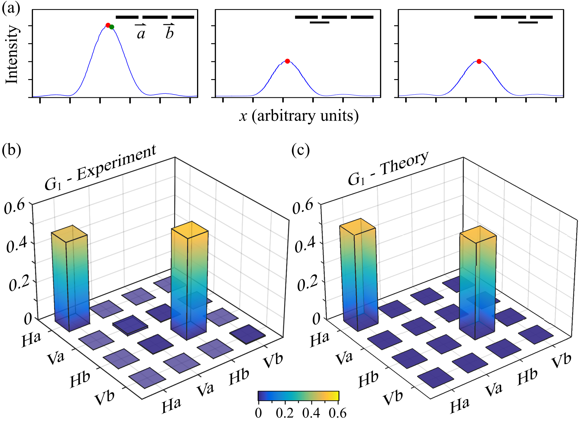
To fully characterize the field coherence across the spatial and polarization DoFs, we measure $\mathbf{G}_{1}$ via OCmT ^{7; 8}, which requires 16 measurements to reconstruct $\mathbf{G}_{1}$. Since 4 polarization projections are required to identify $\mathbf{G}_{\mathrm{p}}$ and 4 spatial projections are required to determine $\mathbf{G}_{\mathrm{s}}$ for a scalar field, $4\times 4$ linearly independent combinations of these spatial and polarization projections are necessary to reconstruct $\mathbf{G}$ subject to the constraints of Hermiticity, semi-positiveness, and unity-trace. These measurements are in one-to-one correspondence to those required to reconstruct a two-qubit density matrix in quantum mechanics, a process known as ‘quantum state tomography’ ^{20; 21; 22}. Carrying out these optical measurements (see ⁸ for details), $\mathbf{G}_{1}$ is reconstructed [Fig. 3(b)] and is found to be in good agreement with the theoretical expectation [Fig. 3(c)], with the remaining slight deviations attributable to unequal powers at $\vec{a}^{\prime}$ and $\vec{b}^{\prime}$.

The measured coherency matrix $\mathbf{G}_{1}$ in the $(\vec{a}^{\prime},\vec{b}^{\prime})$-plane yields $S=1.001$, and the reduced spatial and polarization coherency matrices $\mathbf{G}_{\mathrm{s}}^{(\mathrm{r})}$ and $\mathbf{G}_{\mathrm{p}}^{(\mathrm{r})}$ obtained from $\mathbf{G}$ yield $S_{\mathrm{s}}=0.991$, $S_{\mathrm{p}}=0.037$, respectively. The field entropy is thus associated with the spatial DoF and not polarization, resulting in an absence of interference fringes [Fig. 3(a)]. The lack of interference fringes is consistent with the fact that all measures of spatial coherence or double-slit interference fringes for a vector field rely on the cross-correlation matrix ¹⁴ or beam-coherence matrix ²³, $\mathbf{G}_{ab}=\footnotesize{\left(\begin{array}[]{cc}G_{ab}^{\mathrm{HH}}&G_{ab}^{\mathrm{HV}}\\ G_{ab}^{\mathrm{VH}}&G_{ab}^{\mathrm{VV}}\end{array}\right)}$, which is the top right $2\times 2$ block of the coherency matrix $\mathbf{G}$. For example, the degree of coherence proposed by E. Wolf ¹⁴, the degree of electromagnetic coherence ^{15; 16}, the complex degree of mutual polarization ²⁴, the visibility predicted through a generalized form of the Fresnel-Arago law ²⁵, or the maximal visibility obtainable through local unitary transformations ^{17; 18} all predict that the observed visibility will be zero if all the entries in $\mathbf{G}_{ab}$ are zero. Because the measured and theoretically expected $\mathbf{G}_{1}$ has all zero entries in the $\mathbf{G}_{ab}$ block, it follows that interference fringes do not form. We proceed to show that interference fringes nevertheless appear once the coherence has been reversibly converted from polarization to the spatial DoF.

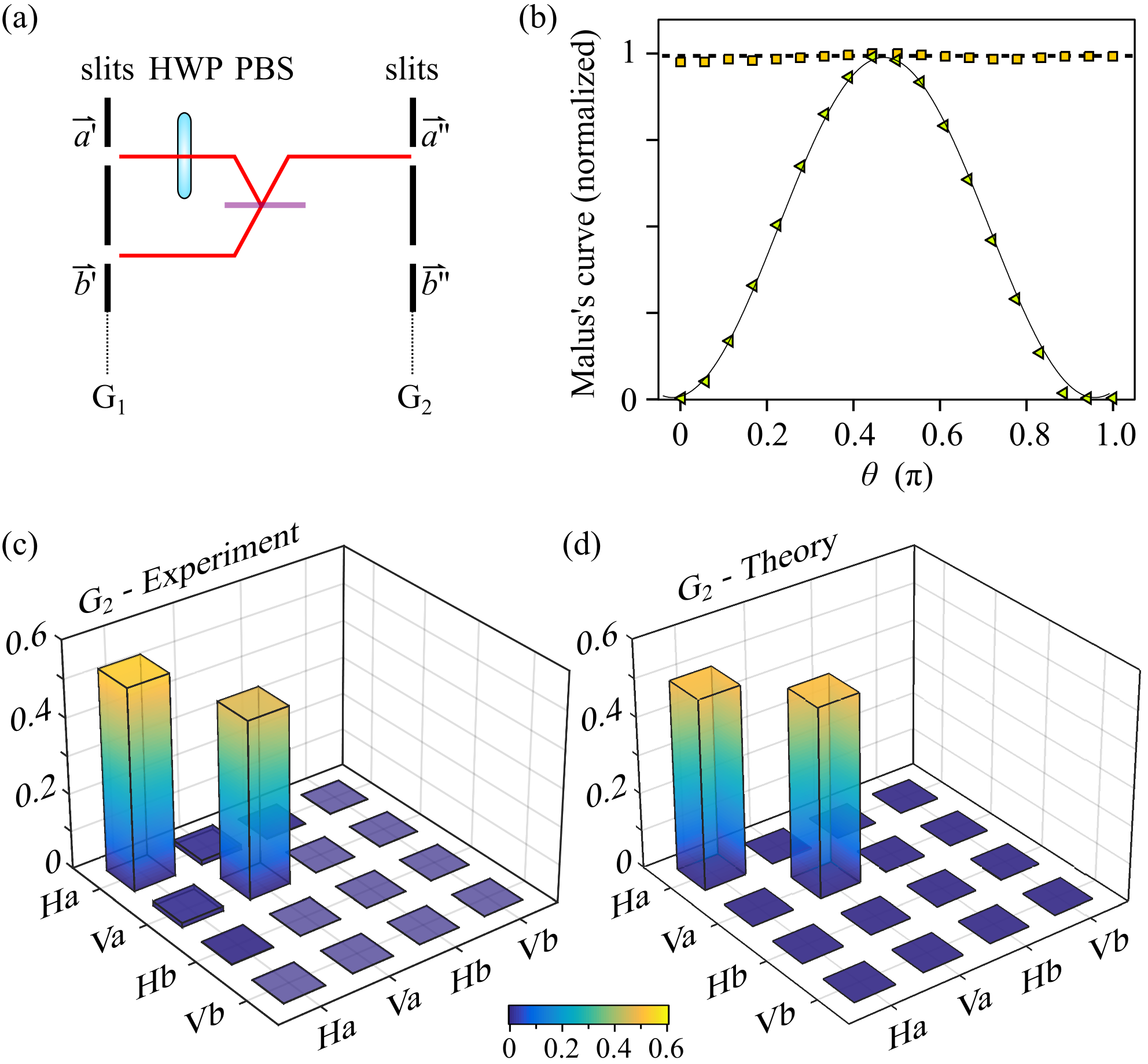
Converting the coherence reversibly from polarization to the spatial DoF entails maximizing the polarization entropy $S_{\mathrm{p}}$ and minimizing the spatial entropy $S_{\mathrm{s}}$ at fixed total entropy $S$. A half-wave plate (HWP) placed after $\vec{b}^{\prime}$ rotates the polarization H$\rightarrow$V, resulting in a new coherency matrix $\mathbf{G}=\tfrac{1}{2}\mathrm{diag}\{1,0,0,1\}$. The fields from $\vec{a}^{\prime}$ and $\vec{b}^{\prime}$ are then directed by mirrors to the two input ports of a PBS (Thorlabs CM1-PBS252), where the V component is transmitted and H is reflected [Fig. 4(a)]. Consequently, the H and V components overlap in the same output port at $\vec{a}^{\prime\prime}$ (minimal power in the other port $\vec{b}^{\prime\prime}$). Note that a PBS is a reversible device: when the two output fields reverse their direction and return to the PBS, the input fields are reconstituted. The field is now unpolarized, which we confirm by registering a flat Malus curve and comparing it to the sinusoidal Malus curve produced by the linearly polarized input fields [Fig. 4(b)]. That is, each incident field on the PBS is linearly polarized, whereas their superposition at the output – with the initial optical power now concentrated in a single path – is randomly polarized. The coherency matrix $\mathbf{G}_{2}$ at $\vec{a}^{\prime\prime}$ and $\vec{b}^{\prime\prime}$ is reconstructed via OCmT [Fig. 4(c)], and is found to be in good agreement with the expected form [Fig. 4(d)]:

From the reconstructed $\mathbf{G}_{2}$ in the $(\vec{a}^{\prime\prime},\vec{b}^{\prime\prime})$-plane, the total entropy is $S=0.997$, but the new values of entropy for the spatial and polarization DoFs are $S_{\mathrm{s}}=0.001$, and $S_{\mathrm{p}}=0.996$, respectively. The entropy has now been converted between the two DoFs. To observe interference fringes, the randomly polarized field at $\vec{a}^{\prime\prime}$ is split symmetrically into two halves by a 50:50 non-polarizing beam splitter to points $\vec{a}$ and $\vec{b}$ [Fig. 5(a)], which can then be overlapped to produce high-visibility fringes. This step does not change the values of $S$, $S_{\mathrm{s}}$, or $S_{\mathrm{p}}$. The $(\vec{a},\vec{b})$-plane is the image plane relayed from the $(\vec{a}^{\prime},\vec{b}^{\prime})$-plane by a lens [Fig. 2(c)]. The coherency matrix $\mathbf{G}_{3}$ in this plane:

The measured $\mathbf{G}_{3}$ reconstructed via OCmT [Fig. 5(b)] is in good agreement with the theoretical expectation [Fig. 5(c)].

Now that we have $G_{ab}^{\mathrm{HH}}+G_{ab}^{\mathrm{VV}}=\tfrac{1}{2}$, the predicted visibility is $V=1$ ¹⁴. Furthermore, because the two DoFs are independent and the field is unpolarized (as is clear from the separable form of $\mathbf{G}_{3}$ in Eq. 27), projecting the polarization on any direction will not affect the high visibility [Fig. 5(d)]. Note that the coherence time of the field is determined by its spectral bandwidth, and observing the fringes [Fig. 5(d)] requires introducing a relative delay in the path of the fields from $\vec{a}$ or $\vec{b}$ before overlapping them [delay line 2 in Fig. 2(c)]. The variation in the measured visibility with introduced relative time delay corresponds to the expected field coherence time $\approx 100$ fs (coherence length $\approx 30$ $\mu$m) [Fig. 5(e)].

The ability to redistribute or reallocate the field entropy $S$ between the DoFs can be exploited in protecting a DoF from the deleterious impact of a randomizing medium. Consider a depolarizing medium represented by a Mueller matrix $\hat{M}=\mathrm{diag}\{1,0,0,0\}$ that converts any state of polarization into a completely unpolarized state. The initial field $\mathbf{G}_{1}$ [Fig. 3(b,c)] would be converted into the incoherent unpolarized field $\mathbf{G}^{\prime}_{1}=\tfrac{1}{4}\mathrm{diag}\{1,1,1,1\}$ upon traversing this medium with $S_{\mathrm{p}}\rightarrow 1$, such that $S\rightarrow 2$. If, however, coherence is first reversibly converted from the spatial DoF to polarization ($S_{\mathrm{p}}\rightarrow 1$ and $S_{\mathrm{s}}\rightarrow 0$), then traversing a depolarizing medium cannot increase $S_{\mathrm{p}}$, and the field is thus left unchanged. Subsequently, the coherence-conversion can be reversed and a polarized field retrieved after emerging from the depolarizing medium without loss of energy.

We have carried out the proof-of-concept experiment depicted in Fig. 6(a) where we place a depolarizer or polarization scrambler in the path of the field $\mathbf{G}_{2}$ in the $(\vec{a}^{\prime\prime},\vec{b}^{\prime\prime})$-plane. The polarization scrambler is implemented by rotating a HWP. The CCD camera exposure time is increased to 10 s, corresponding to the rotation time of the waveplate, to capture the averaged interference pattern in a single shot. The Mueller matrix associated with a polarization scrambler is $\hat{M}=\mathrm{diag}\{1,0,0,0\}$. The visibility observed after the $(\vec{a},\vec{b})$-plane remains high. This result can be modeled theoretically by first noting that a unitary transformation $\hat{U}$ transforms the field according to $\mathbf{G}_{2}\rightarrow\mathbf{G}^{\prime}_{2}=\hat{U}\mathbf{G}_{2}\hat{U}^{{\dagger}}$, where $\hat{U}$ is a $4\times 4$ unitary transformation that spans the spatial and polarization DoFs. If the device in question impacts the two DoFs independently, then $\hat{U}=\hat{U}_{\mathrm{s}}\otimes\hat{U}_{\mathrm{p}}$, where $\hat{U}_{\mathrm{s}}$ and $\hat{U}_{\mathrm{p}}$ are $2\times 2$ unitary transformations for the spatial and polarization DoFs, respectively. The impact of a randomizing but energy-conserving transformation can be modeled as a statistical ensemble of unitary transformations ^{26; 27; 28}. The transformation of $\mathbf{G}_{2}$ upon traversing a polarization scrambler can be expressed as

where $\hat{\mathbb{I}}$ is the $2\times 2$ identity matrix and the ensemble $\{U_{\mathrm{p}}^{(j)}\}$ comprises with equal probabilities $p_{j}=\tfrac{1}{4}$ the Jones matrices: $\tfrac{1}{\sqrt{2}}\footnotesize{\left(\begin{array}[]{cc}1&-1\\ 1&1\end{array}\right)}$, $\tfrac{1}{\sqrt{2}}\footnotesize{\left(\begin{array}[]{cc}1&1\\ -1&1\end{array}\right)}$, $\footnotesize{\left(\begin{array}[]{cc}1&0\\ 0&-1\end{array}\right)}$, $\footnotesize{\left(\begin{array}[]{cc}0&1\\ 1&0\end{array}\right)}$, which correspond to polarization rotations of $\pm 45^{\circ}$ in the H-V basis, and a HWP in the H-V basis and rotated by $45^{\circ}$. Substituting the ensemble $\{\hat{U}_{\mathrm{p}}^{(j)}\}$ into Eq. 28 yields $\mathbf{G}_{2}^{\prime}=\mathbf{G}_{2}$, which entails that the high-visibility seen in Fig. 5(d) should be retained, as confirmed in Fig. 6(a). In other words, $\mathbf{G}_{2}$ is invariant with regards to any polarization randomization.

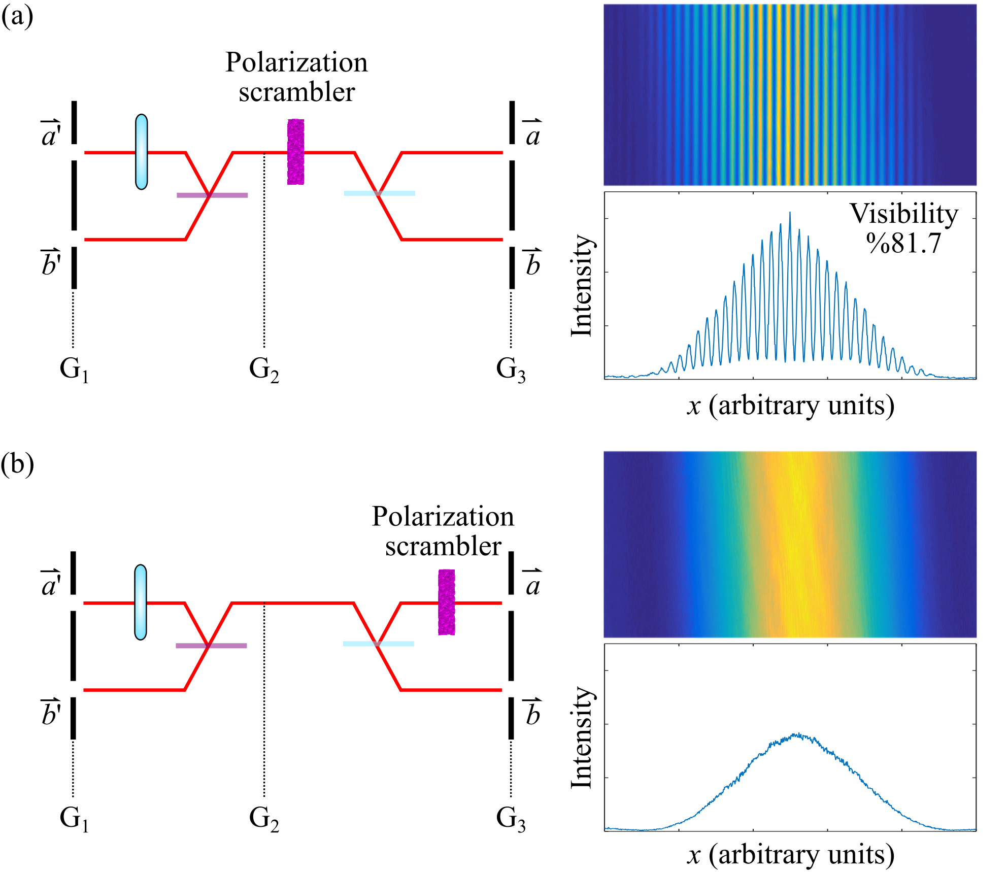
If the polarization scrambler is position-dependent, the coherency matrix $\mathbf{G}_{2}$ will no longer be invariant under randomization (because the spatial and polarization DoFs become coupled). In the experiment illustrated in Fig. 6(b), the polarization scrambler is placed at $\vec{a}$ in the plane of $\mathbf{G}_{3}$. The spatial-polarization transformation of $\mathbf{G}_{3}$ takes the form

where we have $\hat{\Lambda}_{a}=\footnotesize{\left(\begin{array}[]{cc}1&0\\ 0&0\end{array}\right)}$ and $\hat{\Lambda}_{b}=\footnotesize{\left(\begin{array}[]{cc}0&0\\ 0&1\end{array}\right)}$, resulting in $\mathbf{G}_{3}^{\prime}=\tfrac{1}{2}\hat{\mathbb{I}}\otimes\tfrac{1}{2}\hat{\mathbb{I}}=\tfrac{1}{4}\mathrm{diag}\{1,1,1,1\}$; that is, an unpolarized and spatially incoherent field with maximal entropy $S=2$ is produced. No fringes will appear in this case [Fig. 6(b)].

To facilitate the analysis of the coherence of optical fields encompassing multiple DoFs, it is becoming increasingly clear that the mathematical formalism of multi-partite quantum mechanical states is most useful ^{29; 5; 6}. The underlying foundation for this utility is the analogy between the mathematical description used in these domains. The Hilbert space of a multi-partite system is the tensor product of the Hilbert spaces of the single-particle subsystems. In classical optics, the multiple DoFs of a beam are described in a linear vector space having formally the structure of a tensor product of the linear vector spaces of the individual DoFs. In the quantum setting, pure multi-partite states that cannot be separated into products of single-particle states are said to be entangled; whereas in the classical setting, fields in which the DoFs cannot be separated are now being called ‘classically entangled’ ⁶, coherence can be viewed as a ‘resource’ that may be reversibly converted from one DoF of the beam to another, just as entanglement is a resource shared among multiple quantum particles. There is a critical difference though between the quantum and classical settings. Entanglement between initially separable particles requires nonlocal operations of particle-particle interactions (which are particularly challenging for photons ³⁰); on the other hand, entangling operations that couple different DoFs of a beam are readily available in classical optics. Adopting this information-driven standpoint has led to a host of novel opportunities and applications. For example, Bell’s measure, originally developed for ascertaining nonlocality, becomes a useful in quantifying the coherence of a multi-DoF beam and assessing the resources required to synthesize a beam of given characteristics ⁶; beams in which spatial modes and polarization are classically entangled have been shown to enable fast particle tracking ³¹ and full Mueller characterization of a sample ^{32; 33}; and introducing spatio-temporal spectral correlations leads to propagation-invariant pulsed optical beams ^{34; 35}.

We have demonstrated – for the first time to the best of our knowledge – the ‘conversion’ or transformation of coherence from one DoF of an optical field to another; namely, from polarization to the spatial DoF. Starting from a field that is spatially incoherent but polarized, we redirect the statistical fluctuations from space towards polarization, resulting in an unpolarized field that is spatially coherent – reversibly, without losing optical energy along the way. Specifically, the 1 bit of entropy characterizing the spatial DoF was removed and added instead to the initially zero-entropy polarization. Entropy-engineering of partially coherent optical fields can open the path to a variety of possible future extensions and applications with regards to optimizing the interaction of optical fields with disordered media.

References

- Mandel and Wolf (1995) L. Mandel and E. Wolf, Optical Coherence and Quantum Optics (Cambridge Univ. Press, Cambridge, 1995).
- Zernike (1938) F. Zernike, Physica 5, 785 (1938).
- Born and Wolf (1999) M. Born and E. Wolf, Principles of Optics (Cambridge Univ. Press, Cambridge, 1999).
- Brosseau (1998) C. Brosseau, Fundamentals of Polarized Light (Wiley, New York, 1998).
- Qian and Eberly (2011) X.-F. Qian and J. H. Eberly, Opt. Lett. 36, 4110 (2011).
- Kagalwala et al. (2013) K. H. Kagalwala, G. Di Giuseppe, A. F. Abouraddy, and B. E. A. Saleh, Nat. Photon. 7, 72 (2013).
- Abouraddy et al. (2014) A. F. Abouraddy, K. H. Kagalwala, and B. E. A. Saleh, Opt. Lett. 39, 2411 (2014).
- Kagalwala et al. (2015) K. H. Kagalwala, H. E. Kondakci, A. F. Abouraddy, and B. E. A. Saleh, Sci. Rep. 5, 15333 (2015).
- Wolf (2007) E. Wolf, Introduction to the Theory of Coherence and Polarization of Light (Cambridge Univ. Press, Cambridge, 2007).
- Al-Qasimi et al. (2007) A. Al-Qasimi, O. Korotkova, D. James, and E. Wolf, Opt. Lett. 32, 1015 (2007).
- Abouraddy (2017) A. F. Abouraddy, Opt. Express , unpublished (2017).
- Brosseau and Dogariu (2006) C. Brosseau and A. Dogariu, in Progress in Optics Vol. 49, edited by E. Wolf (Elsevier, Amsterdam, 2006) Chap. 4, pp. 315–380.
- Gori et al. (2006) F. Gori, M. Santarsiero, and R. Borghi, Opt. Lett. 31, 858 (2006).
- Wolf (2003) E. Wolf, Phys. Lett. A 312, 263 (2003).
- Tervo et al. (2003) J. Tervo, T. Setälä, and A. T. Friberg, Opt. Express 11, 1137 (2003).
- Setälä et al. (2004) T. Setälä, J. Tervo, and A. T. Friberg, Opt. Lett. 29, 328 (2004).
- Gori et al. (2007) F. Gori, M. Santarsiero, and R. Borghi, Opt. Lett. 32, 588 (2007).
- Martínez-Herrero and Mejías (2007) R. Martínez-Herrero and P. M. Mejías, Opt. Lett. 32, 1471 (2007).
- Peres (1995) A. Peres, Quantum Theory: Concepts and Methods (Kluwer Academic Publishers, Dordrecht, 1995).
- Wootters (1990) W. K. Wootters, in Complexity, Entropy, and the Physics of Information, SFI Studies in the Sciences of Complexity, Vol. VIII, edited by W. H. Zurek (Addison-Wesley, Reading, 1990) pp. 39–46.
- James et al. (2001) D. F. V. James, P. G. Kwiat, W. J. Munro, and A. G. White, Phys. Rev. A 64, 052312 (2001).
- Abouraddy et al. (2002) A. F. Abouraddy, A. V. Sergienko, B. E. A. Saleh, and M. C. Teich, Opt. Comm. 201, 93 (2002).
- Gori (1998) F. Gori, Opt. Lett. 23, 241 (1998).
- Ellis and Dogariu (2004) J. Ellis and A. Dogariu, Opt. Lett. 29, 536 (2004).
- Mujat et al. (2004) M. Mujat, A. Dogariu, and E. Wolf, J. Opt. Soc. Am. A 21, 2414 (2004).
- Kim et al. (1987) K. Kim, L. Mandel, and E. Wolf, J. Opt. Soc. Am. A 4, 433 (1987).
- Gil (2000) J. J. Gil, J. Opt. Soc. Am. A 17, 328 (2000).
- Gamel and James (2011) O. Gamel and D. F. V. James, Opt. Lett. 36, 2821 (2011).
- Simon et al. (2010) B. N. Simon, S. Simon, F. Gori, M. Santarsiero, R. Borghi, N. Mukunda, and R. Simon, Phys. Rev. Lett. 104, 023901 (2010).
- Venkataraman et al. (2013) V. Venkataraman, K. Saha, and A. L. Gaeta, Nat. Photon. 7, 138 (2013).
- Berg-Johansen et al. (2015) S. Berg-Johansen, F. Töppel, B. Stiller, P. Banzer, M. Ornigotti, E. Giacobino, G. Leuchs, A. Aiello, and C. Marquardt, Optica 2, 864 (2015).
- Töppel et al. (2014) F. Töppel, A. Aiello, C. Marquardt, E. Giacobino, and G. Leuchs, New J. Phys. 16, 073019 (2014).
- Tripathi and Toussaint (2009) S. Tripathi and K. C. Toussaint, Opt. Express 17, 21396 (2009).
- Kondakci and Abouraddy (2016) H. E. Kondakci and A. F. Abouraddy, Opt. Express 24, 28659 (2016).
- Parker and Alonso (2016) K. J. Parker and M. A. Alonso, Opt. Express 24, 28669 (2016).