[a]M. A. Petri [b,c]A. D. M. Valois
Dense and magnetized QCD from imaginary chemical potential
Abstract
In this work, we computed the equation of state of dense QCD in the presence of background magnetic fields using lattice QCD simulations at imaginary baryon chemical potential. Our simulations include 2+1+1 flavors of stout-smeared staggered fermions with masses at the physical point and a tree-level Symanzik-improved gauge action. Using several expansion schemes, we tuned our simulation parameters such that the equation of state satisfies strangeness neutrality and isospin asymmetry constraints, which are relevant to the phenomenology of heavy-ion collisions. Our results suggest a strong change in the equation of state due to the magnetic field, in particular, around the crossover temperature. A continuum extrapolation of our data is still needed for future applications of our equation of state to heavy-ion-collision phenomenology.
1 Introduction
It is widely believed that strongly interacting matter existed as a Quark-Gluon Plasma (QGP) during the first microseconds of the Universe, where quarks and gluons were subjected to high temperatures and densities. During that epoch, the so-called electroweak phase transition may have generated magnetic fields comparable with the typical energy scale of the strong interactions [1]. In the present Universe, this strongly interacting phase of matter is believed to exist inside the core of neutron stars, some of which also show strong magnetic fields. The study of such extreme environments in the lab has been pioneered by experiments of Heavy-Ion Collisions (HICs). These experiments also account for the strongest magnetic fields ever produced on Earth. In peripheral collisions, for instance, the motion of charged particles generates field lines that reinforce each other at the center of the collision. The sizeable impact of such fields on experimentally measurable observables has been recently seen by the STAR Collaboration [2]. In phenomenological studies, theoretical estimates indicate that magnetic fields reach – for typical Au+Au collisions – at RHIC energies [3] and – for typical Pb+Pb collisions – at LHC energies [4].
Besides strong magnetic fields, high densities can also be created in HICs. High-density strongly interacting matter produced in relativistic collisions is relevant not only for ongoing experiments, such as RHIC, but also for future ones, like NICA and FAIR. From a theoretical viewpoint, high densities also provide a path to understanding the different phases of the strong interactions via its underlying microscopic theory: Quantum Chromodynamics (QCD).
At vanishing density, the QCD phase transition is a smooth crossover [5], whereas at high densities it is conjectured to become first order. The presence of a first-order line would imply the existence of a second-order transition point, known as a Critical Endpoint (CEP). This hypothesis has been corroborated by analytical approaches, such as the Functional Renormalization Group [6], Dyson-Schwinger equations [7], holographic models [8], etc.
On the one hand, first-principles numerical simulations of the strong interactions on a lattice – Lattice QCD (LQCD)– successfully account for all non-perturbative features of QCD at vanishing and low densities. On the other hand, the approach becomes unfeasible at moderate and high densities due to the sign (or complex action) problem. Although various techniques have been used to circumvent this issue (see Ref. [9] for a recent review), to this day, the determination of the phase structure of QCD at high from first principles remains a widely open problem.
Theoretically, one can extend the QCD phase diagram to the (imaginary) domain, where lattice simulations are sign-problem-free. Interestingly, at imaginary , the phase diagram has a second-order transition point called Roberge-Weiss CEP [10]. Also, the QCD phase diagram in the - plane is directly accessible within lattice simulations. In the presence of a magnetic field, the QCD crossover becomes sharper and the transition temperature is lowered, suggesting that the crossover would eventually become a first-order transition starting at a CEP. Moreover, lattice simulations of asymptotically strong magnetic fields found further indication for this scenario [11], thus supporting previous expectations based on generic arguments [12] (see also Ref. [13]). Recent LQCD results constrained this CEP to the region: , [14]. The impact of magnetic fields on the Roberge-Weiss CEP has also been studied using LQCD, where the findings indicate that this point approaches the - plane, thus opening the possibility of a connection between the two critical points [15].
Another way of probing thermodynamic features of QCD is via the Equation of State (EoS). Moreover, knowing the EoS as a function of thermodynamic variables (, , , etc.) is essential to model the hydrodynamic evolution of relativistic collisions across the phase diagram. In this regard, the present knowledge of the interplay between finite densities and magnetic fields is limited. Currently, the EoS at is known from LQCD in a broad range of temperatures at vanishing with 2+1 flavors [16, 17], as well as at non-vanishing with 2+1 flavors [18], and 2+1+1 flavors [19]. At , the EoS has been calculated with 2+1 flavors at non-zero but vanishing strangeness chemical potential [20]. For a recent review on lattice investigations of the phase diagram and the EoS at nonzero magnetic fields, see Ref. [21].
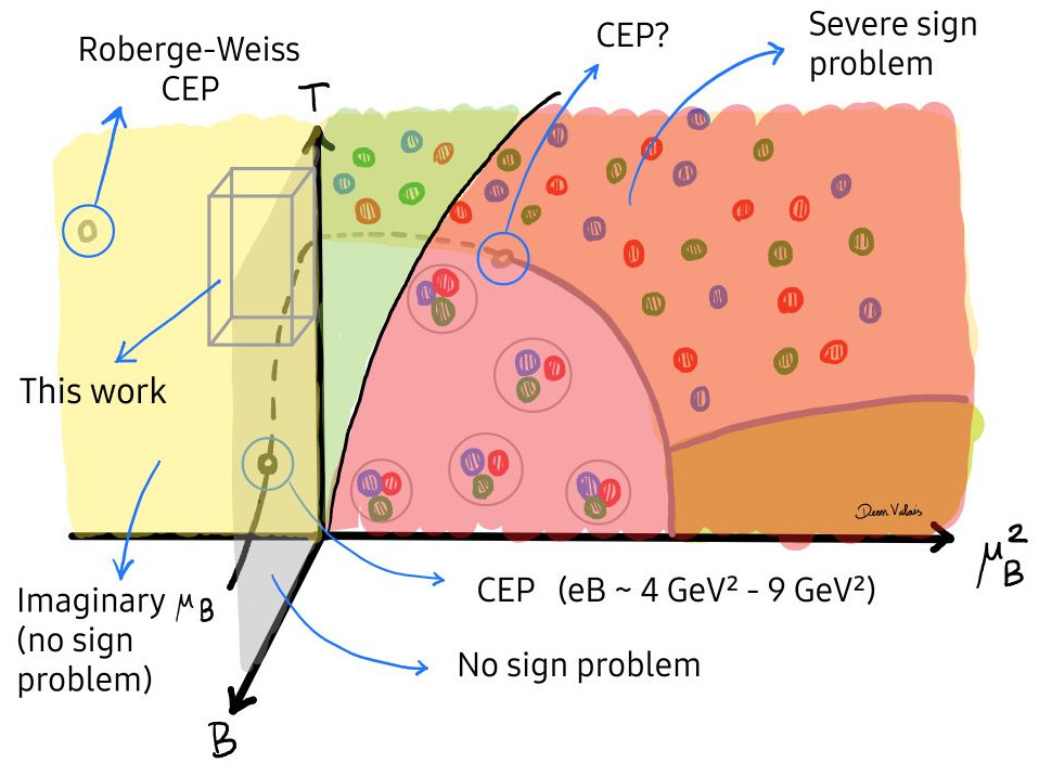
Hence, in this proceedings article, we aim to shed light on the EoS of dense and magnetized QCD matter with four dynamical quark flavors. Our method of choice to circumvent the sign problem is analytic continuation from simulations at imaginary , thus extending our previous work [22], where we carried out simulations at vanishing . Our EoS is taken along a trajectory satisfying two constraints motivated by the HIC setup, namely, strangeness neutrality and isospin asymmetry. Our discussions revolve around two main quantities: the chemical potentials and required by our constraints, and the leading-order behavior of the EoS. We show that the magnetic field significantly impacts the latter, in particular, near the crossover temperature. In Fig. 1, we illustrate the conjectured QCD phase diagram in the -- space and indicate where we carried out simulations.
This article is organized as follows: In Sec. 2, we describe the simulation setup, including our lattice action and simulation parameters. In Sec. 3, we introduce the definitions of the observables we compute as well as the constraints that we impose on our EoS. This is followed by Sec. 4, in which we explain our method to fulfill the constraints at non-zero chemical potential. Finally, in Secs. 5 and 6, we present our results and conclusions, respectively.
2 Simulation setup
In the fermion sector, we employed flavors of rooted-staggered fermions with four stout-smearing steps and masses tuned to the physical point. For details on our Line of Constant Physics (LCP), see Ref. [23]. In the gauge sector, we used the tree-level Symanzik-improved gauge action [24]. In this setup, we generated gauge configurations on a lattice for various temperatures, imaginary chemical potentials, and magnetic field strengths. We varied the temperature via the inverse gauge coupling according to , where is the lattice spacing and the number of sites in the temporal extent, and the imaginary chemical potential via , with . We scanned the temperature in the range – MeV in steps of MeV, and the following chemical potentials: . Finally, without loss of generality, we considered a uniform magnetic field pointing in the direction. To simulate the magnetic field, we multiplied the gluon links by the corresponding U(1) factors at each lattice site. For the exact form of these factors, see [25].
In a finite volume, the magnetic field flux satisfies the following quantization condition
| (1) |
where and are the lattice extents along the and directions, respectively. Due to QED-related charge- and magnetic-field renormalizations, the amplitude of the field is typically expressed in terms of the renormalization-group-invariant quantity . In this fashion, we simulated GeV2 magnetic fields, which encompass the values expected in the physical systems described in Sec. 1. To achieve the desired values of – given that the change of flux can only be carried out in integer steps – for each of the aforementioned field strengths, we simulated two values of that surround the desired value. Thus, we obtained results at the desired using a linear interpolation.
3 Equation of state and constraints
Here, we give the definitions of the observables that we compute. Let us start by introducing the pressure in terms of the grand canonical partition function of QCD in the rooted-staggered formalism
| (2) |
where is the spatial volume, , and are the reduced chemical potentials in the quark basis. Notice that we do not include the charm chemical potential although the charm quark is dynamically included in our simulations. Moreover, we define the quark-number susceptibilities as
| (3) |
These susceptibilities can be converted to the physical basis – involving baryon, charge, and strangeness quantum numbers – yielding, for instance, the following number densities
| (4) |
Using these quantities, we can now introduce the constraints that we impose on the EoS, namely,
| (5) |
These are known respectively as strangeness neutrality and isospin asymmetry. The ratio and the value of are chosen to match the experimental values expected for the byproducts of typical Pb+Pb collisions, for instance. These constraints imply that there is only one independent chemical potential, since and can be expressed in terms of .
Taking these constraints into account, we can compute the pressure change at finite chemical potential along the line of strangeness neutrality and isospin asymmetry using the integral method
| (6) |
where was introduced in (2). In terms of the number densities (4), the total derivative of the pressure with respect to can be written as
| (7) |
where the partial derivatives of and with respect to appear due to the constraints. Knowing the right-hand side of Eq. (7) allows us to compute the pressure shift via the integral method. Next, we discuss how to tune the charge and strangeness chemical potentials in terms of such that strangeness neutrality and isospin asymmetry are fulfilled.
4 Matching the experimental conditions
This section focuses on realizing the experimental conditions of HICs on the lattice. One way is to precisely tune the simulation parameters. Another way is to compute additional derivatives and extrapolate to strangeness neutrality afterwards. To avoid large computational costs during tuning while still simulating close to the strangeness neutral case to avoid a complicated extrapolation, we combine both. To simulate close to strangeness neutrality at we estimate and from all simulations up to . The shift into exact strangeness neutrality, which is a small difference in and . The determination of the shift is performed after the simulation. We determine the new simulation parameters at by performing extrapolations in using Taylor-expansions up to a certain order, depending on the number of simulation in direction already performed. This means we make an ansatz such as Eq. (8), where are the parameters we want to determine.
| (8) |
To estimate systematic effects we calculate the parameters using different approaches. Combining simulations with estimated parameters with a correction to strangeness neutrality afterwards has the advantage that we keep the computational cost for both the simulation and analysis in balance with low statistical uncertainties. The small deviation of the estimated parameters from the true ones in strangeness neutrality ensures that by performing a linear extrapolation we can calculate the shift and in the chemical potentials to reach the experimental conditions while keeping the impact on the uncertainties in our observables as small as possible. The susceptibilities in strangeness neutrality after the shift, denoted as read as written in Eq. (9).
| (9) |
We will now discuss the different approaches to estimating the chemical potentials for the simulations
4.1 Algebraic Determination
For the algebraic procedure, let us start by taking the derivative of Eq. (8) with respect to .
| (10) |
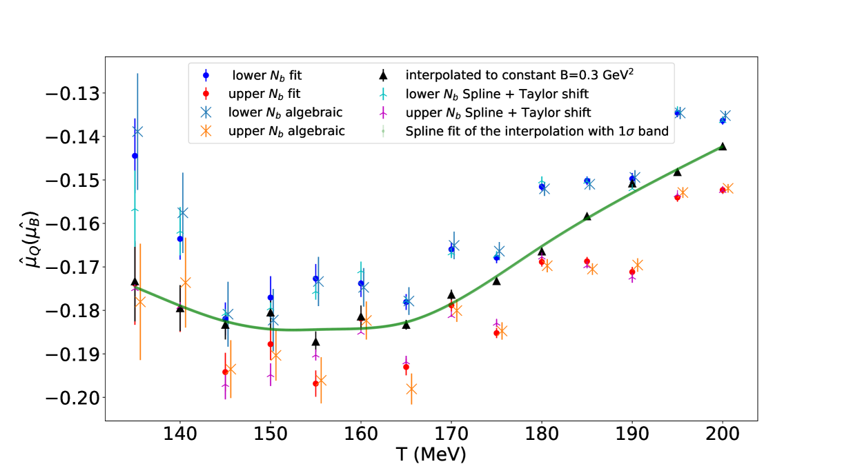
Taking we see that the coefficient is given by . Since the simulation at is already in strangeness neutrality, we have a given parameter for the Taylor expansion of Eq. (8). The expansion to the first order can be used to estimate the . For the determination of higher order parameters, one can use the measurements of both as well as higher order derivatives of the expansion, in order to solve algebraically for the parameters . The advantage of this procedure is its computational simplicity and efficiency, which provides a fast result. However, a notable drawback is that higher-order parameters often have large statistical uncertainties, which can significantly impact the results and lead to larger overall errors, particularly when the higher-order parameters are compatible with zero. This effect is particularly pronounced at low temperatures, as shown in Fig. 2, where obtaining a sufficient amount of reliable statistics is also more computationally expensive.
4.2 Fit procedure
Another approach would be to perform a global fit and minimize . For this, we account for the fact that higher-order terms in Eq. (8) are associated with larger statistical uncertainties. We fit the value of in strangeness neutrality as well as the first derivative . The model used is the Taylor expansion (8). The expansion order must be adjusted to balance the number of degrees of freedom with the fact that higher-order terms tend to have larger uncertainties, which can make parameters indistinguishable from zero within errors.
4.2.1 Incorporating the line of constant magnetic field
As an additional step to further reduce statistical uncertainties, we leverage the fact that the desired values lie on a line of constant magnetic field. We perform a spline interpolation of the values interpolated to the line of constant magnetic field of as well as for their discrete derivatives with respect to changes in . Using these interpolated values and their derivatives, we apply a Taylor expansion (linear in ) to extrapolate the values from the line of constant magnetic field to the nearest integer values of above and below. This is to reduce systematic effects due to the different distances from the two integer values of to the constant magnetic field value for . In Fig. 2 we observe that this approach yields even smaller statistical uncertainties compared to the simple fit results at the integer values.
4.3 Conclusion of the methods
The results for of the described methods are shown in Fig. 2. The temperature scan with both values for the different at each temperature for the simulation for at an external magnetic field value around GeV2 is shown. For better visibility, a small shift in the temperature axis was inserted for the different methods. The methods agree within errors for most temperatures. In the low-temperature regime, the overall error is larger for all methods than for the high temperatures. Consequently, the chosen values for the next simulation originate from the spline fit routine, combined with the Taylor expansion to map the results back to integer-valued .
5 Results
5.1 Chemical potentials
In this section, we focus on the impact of the extrapolation to , as well as the physical interpretation of our findings in the presence of an external magnetic field for simulations with a chemical potential. First, we examine the difference between the baryon number calculated using Eq. (3), measured directly after the simulation, and the baryon number after imposing strangeness neutrality and isospin asymmetry calculated via Eq. (9), as shown in Fig. 3.
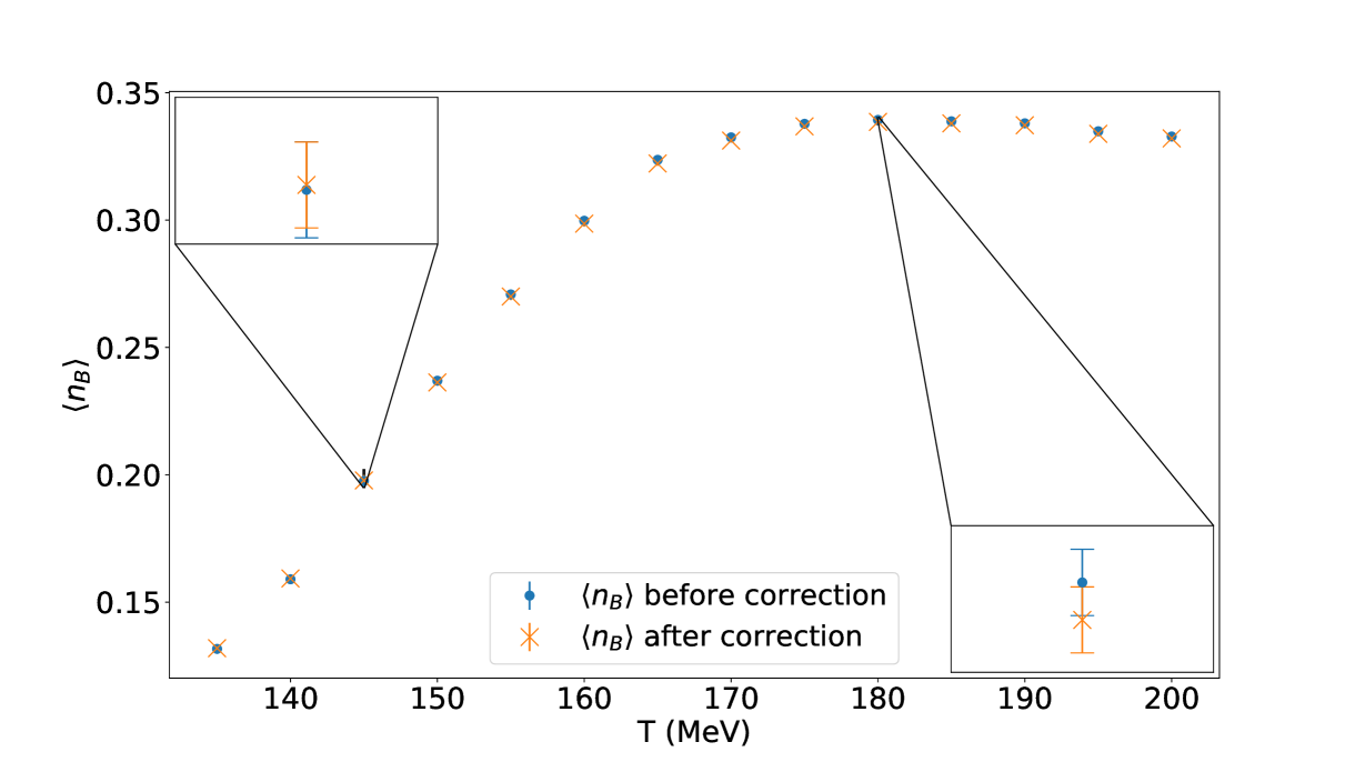
The figure confirms two predictions. First of all, we observe that the shift we have to take in order to reach strangeness neutrality is within the errors of the measurements without the shift. Secondly, we observe that the error is manageable – it does not obscure the trend of the data with respect to temperature – and remains stable with the shift. This demonstrates that our procedure is sufficient for determining new simulation parameters, where the shift to strangeness neutrality can be effectively handled using a linear Taylor expansion.
At the next point, we would like to study how an external magnetic field impacts the chemical potentials, and why. For that let us take a look at the choice of the charge and strange chemical potential per baryon chemical potential for different external magnetic fields in Figs. 4(a) and 4(b).
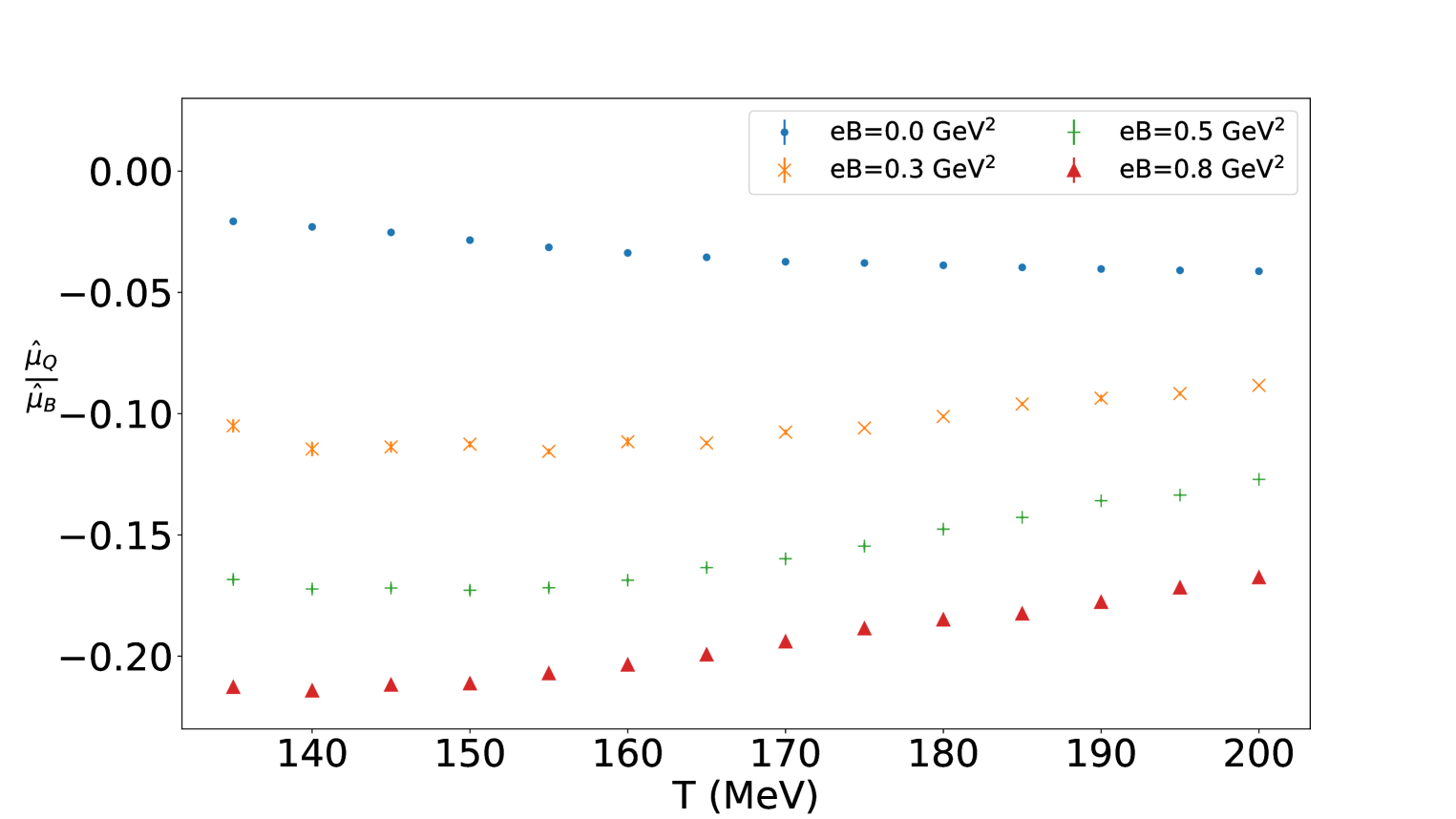
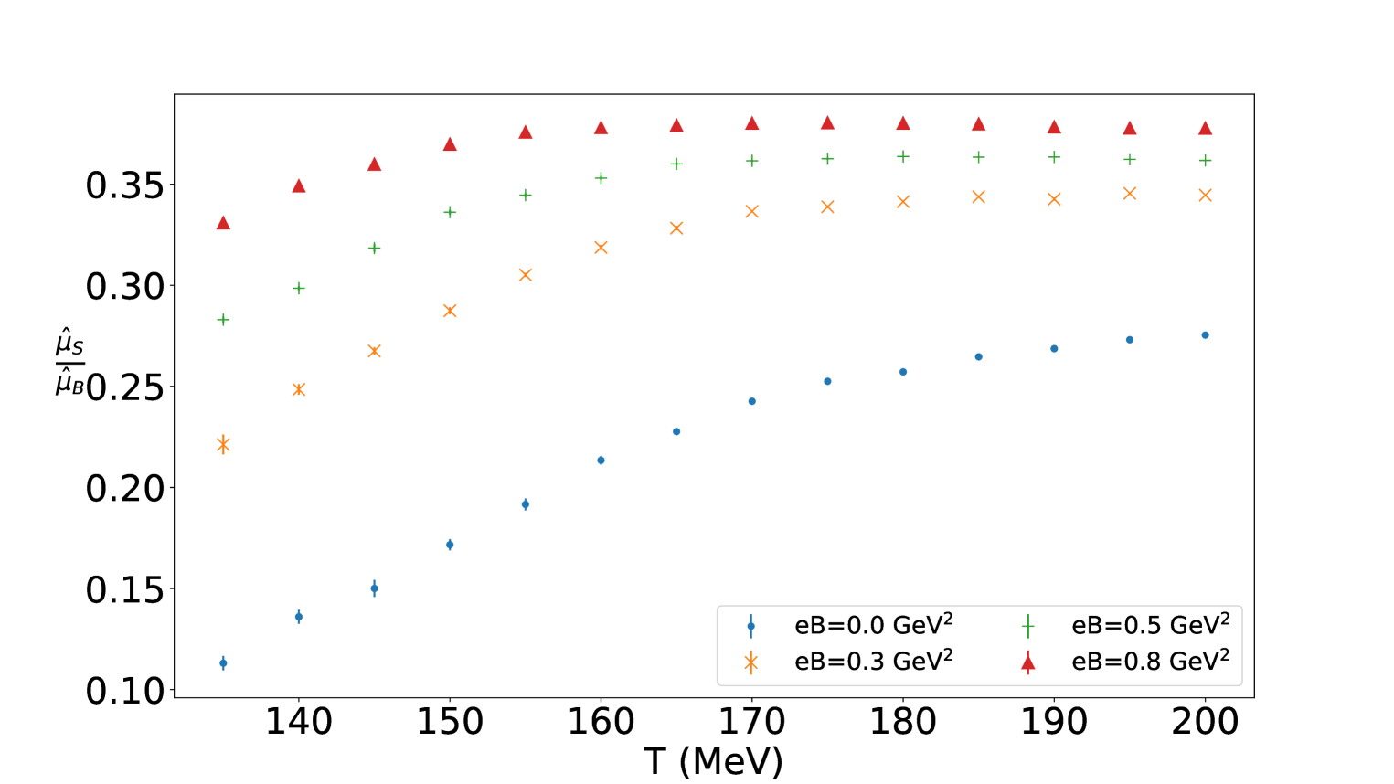
First, let us focus on the Fig. 4(a). The overall negative value of originates from the fact that the constraint (5) for requires an excess of down quarks over up quarks and, therefore, a suppression of electric charge. According to the figure, this negative value decreases consistently throughout the temperature range as the magnetic field grows. To understand this behavior intuitively, let us focus on the low-temperature regime, where the baryon number and electric charge are mostly carried by protons and neutrons. The effect we observe can be attributed to the coupling of these particles to the magnetic field. The lowest energy state is affected by the magnetic field via the spin and the angular momentum terms. Taking into account both of these couplings, together with the proton and neutron gyromagnetic ratios [26], the ground state energies for both hadrons reduce by similar amounts, thus enhancing the abundance of protons and neutrons similarly and pushing the system towards isospin symmetry. To compensate for this, the charge chemical potential needs to be reduced further. This qualitative behavior may be quantified more using the standard hadron resonance gas model approach considered at nonzero magnetic field [27] and nonzero chemical potentials [28, 29]. A similar argument applies to the strange chemical potential shown in Fig. 4(b). Here, instead of comparing the gyromagnetic ratios of protons and neutrons, one must examine those of hyperons relative to baryons. This, combined with the requirement of zero net strangeness in the system, leads to a similar conclusion.
5.2 Analytic continuation
Finally, in this section, we present preliminary results from our approach to the analytic continuation of the EoS. Our main observable is shown in Eq. (7), i.e. the total derivative of the pressure with respect to the baryon chemical potential. The analytic continuation procedure was carried out by fitting a multidimensional spline surface to the quantity taking into account the , and directions. The advantage of this particular combination is that, in leading order, this observable is linear in , which permits an extrapolation to the real axis using a linear surface along the direction. Notice that, even though vanishes at , the quantity has a non-zero value there.
The functional form of the spline surface is a fourth-order polynomial in the and directions, whereas it is linear in the direction. This allows us to extract the leading-order behavior of the EoS in the real- axis. In order to account for systematic errors in the spline fit, we stochastically generated multiple sets of node points using a Monte Carlo algorithm, for more details see Refs. [30, 31], where the spline solutions are weighted according to the Akaike criterion [32]. Moreover, to have a more realistic estimation of the systematic effects, we also included spline solutions where the data at were removed from the global fit. In Fig. 5 we show the result of the multidimensional spline fit for different values of the magnetic field.
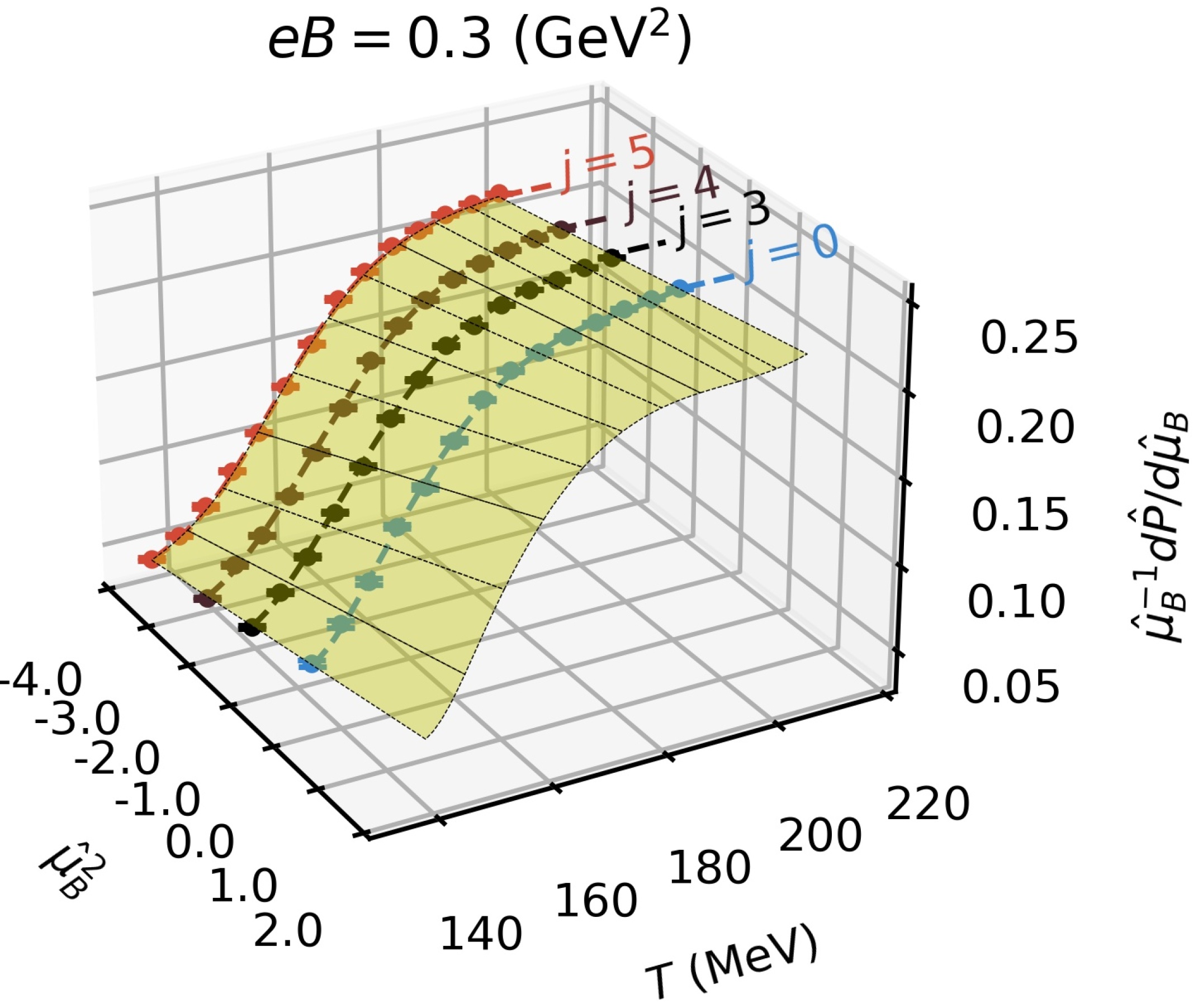
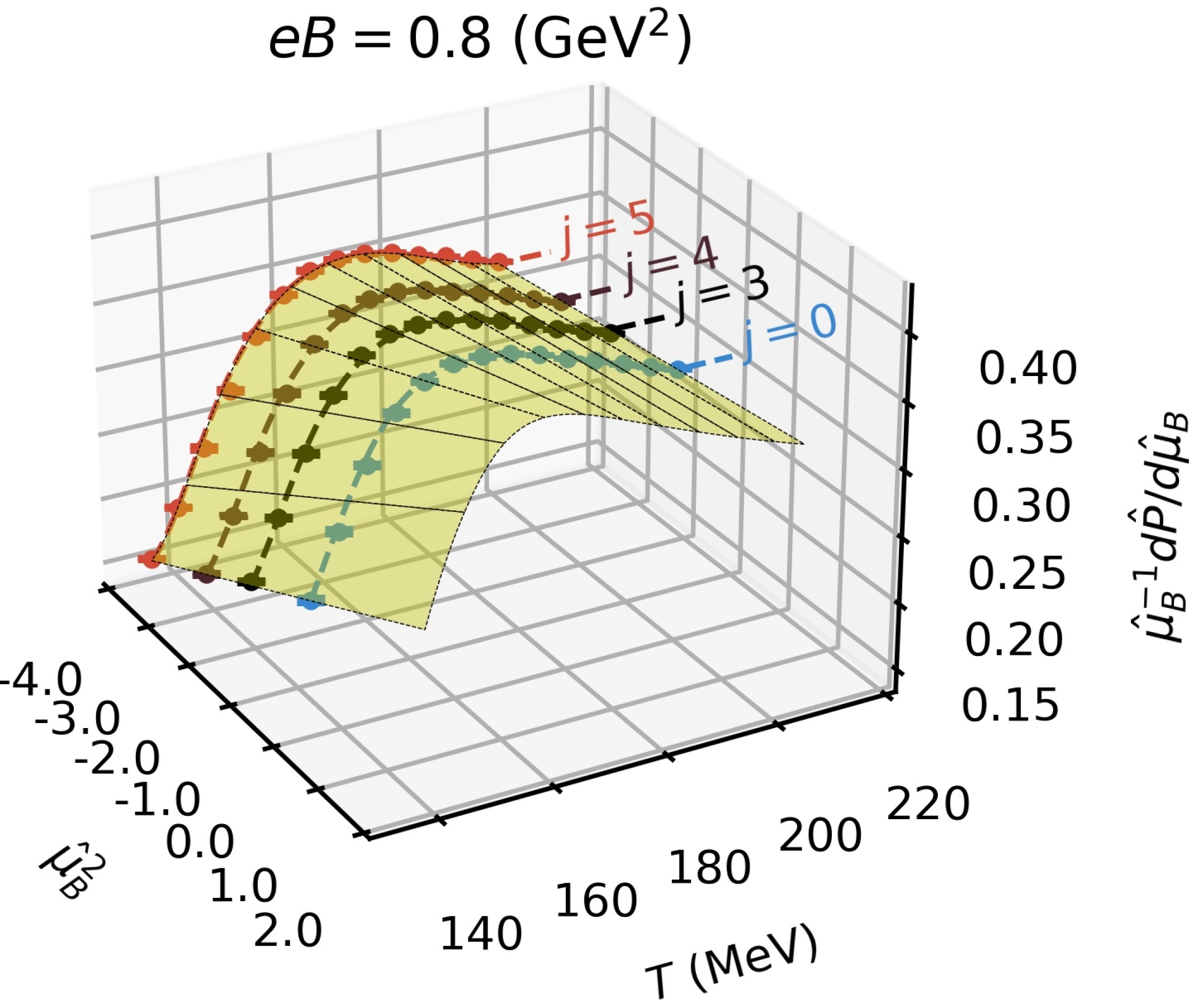
The most striking consequence of the non-zero magnetic field, as seen from the surfaces in Fig. 5, is the bending towards high temperatures, where the data shows a peak structure near the crossover temperature. Moreover, whereas the behavior of is still monotonic at low , it becomes non-monotonic at higher .
6 Conclusions and outlook
In this proceedings article, we investigated the interplay between finite density and nonzero magnetic fields in QCD in the light of observables that can be related to the EoS. We performed simulations at imaginary chemical potential with 2+1+1 dynamical quarks and a physical pion mass. We used different expansion schemes to constrain our simulation parameters to a strangeness-neutral and isospin-asymmetric line, where we defined as the isospin asymmetry ratio. These constraints are motivated by phenomenological expectations in HICs.
Using a multidimensional spline fit, we took the first steps towards the analytic continuation of our data to the real-chemical-potential axis. At this stage, our results show that the magnetic field has a significant impact on the observables, especially around the crossover temperature. Specifically, we observed that the quantity ceased to be monotonic with temperature in the presence of strong enough magnetic fields, namely, for GeV2. This behavior has previously been observed in second-order susceptibilities and in the leading-order coefficient of the EoS [22]. See also Ref. [33] for further discussion about the impact of on these observables.
In order to make contact with continuum QCD physics, the continuum limit of the results presented here must still be carried out, as well as the full analytic continuation of our data. Nevertheless, our current findings reveal interesting features of the impact of strong magnetic fields on hot and dense QCD matter which might be insightful for the modeling of systems where such medium is created: HICs.
Acknowledgments
This work is supported by the MKW NRW under the funding code NW21-024-A. The authors gratefully acknowledge the Gauss Centre for Supercomputing e.V. for funding this project by providing computing time on the GCS Supercomputer SuperMUC-NG at Leibniz Supercomputing Centre. The authors are also grateful to Gergely Markó for discussions that shaped our approach to the results presented here. Moreover, we acknowledge Arpith Kumar and Jin-Biao Gu for helpful discussions on dense and magnetized QCD during this conference. Gergely Endrődi acknowledges funding by the Hungarian National Research, Development and Innovation Office (Research Grant Hungary 150241) and the European Research Council (Consolidator Grant 101125637 CoStaMM).
Acronyms
- CEP
- Critical Endpoint
- EoS
- Equation of State
- HIC
- Heavy-Ion Collision
- LCP
- Line of Constant Physics
- LQCD
- Lattice QCD
- QCD
- Quantum Chromodynamics
- QGP
- Quark-Gluon Plasma
References
- [1] T. Vachaspati, Magnetic fields from cosmological phase transitions, Phys. Lett. B 265 (1991) 258.
- [2] STAR Collaboration, M. I. Abdulhamid et al., Observation of the electromagnetic field effect via charge-dependent directed flow in heavy-ion collisions at the Relativistic Heavy Ion Collider, Phys. Rev. X 14 (2024) 011028, [2304.03430].
- [3] D. E. Kharzeev, L. D. McLerran, and H. J. Warringa, The Effects of topological charge change in heavy ion collisions: ’Event by event P and CP violation’, Nucl. Phys. A 803 (2008) 227, [0711.0950].
- [4] V. Skokov, A. Y. Illarionov, and V. Toneev, Estimate of the magnetic field strength in heavy-ion collisions, Int. J. Mod. Phys. A 24 (2009) 5925, [0907.1396].
- [5] Y. Aoki, G. Endrődi, Z. Fodor, S. D. Katz, and K. K. Szabó, The Order of the quantum chromodynamics transition predicted by the standard model of particle physics, Nature 443 (2006) 675, [hep-lat/0611014].
- [6] W.-j. Fu, J. M. Pawlowski, and F. Rennecke, QCD phase structure at finite temperature and density, Phys. Rev. D 101 (2020) 054032, [1909.02991].
- [7] C. S. Fischer, QCD at finite temperature and chemical potential from Dyson–Schwinger equations, Prog. Part. Nucl. Phys. 105 (2019) 1, [1810.12938].
- [8] M. Hippert, J. Grefa, T. A. Manning, J. Noronha, J. Noronha-Hostler, I. Portillo Vazquez, C. Ratti, R. Rougemont, and M. Trujillo, Bayesian location of the QCD critical point from a holographic perspective, Phys. Rev. D 110 (2024) 094006, [2309.00579].
- [9] C. E. Berger, L. Rammelmüller, A. C. Loheac, F. Ehmann, J. Braun, and J. E. Drut, Complex Langevin and other approaches to the sign problem in quantum many-body physics, Phys. Rept. 892 (2021) 1, [1907.10183].
- [10] A. Roberge and N. Weiss, Gauge Theories With Imaginary Chemical Potential and the Phases of QCD, Nucl. Phys. B 275 (1986) 734.
- [11] G. Endrődi, Critical point in the QCD phase diagram for extremely strong background magnetic fields, JHEP 07 (2015) 173, [1504.08280].
- [12] T. D. Cohen and N. Yamamoto, New critical point for QCD in a magnetic field, Phys. Rev. D 89 (2014) 054029, [1310.2234].
- [13] V. V. Braguta, M. N. Chernodub, A. Y. Kotov, A. V. Molochkov, and A. A. Nikolaev, Finite-density QCD transition in a magnetic background field, Phys. Rev. D 100 (2019) 114503, [1909.09547].
- [14] M. D’Elia, L. Maio, F. Sanfilippo, and A. Stanzione, Phase diagram of QCD in a magnetic background, Phys. Rev. D 105 (2022) 034511, [2111.11237].
- [15] K. Zambello, M. D’Elia, L. Maio, and G. Zanichelli, The Roberge-Weiss endpoint in (+)-flavor QCD with background magnetic fields, PoS LATTICE2024 (2025) 169, [2412.06326].
- [16] S. Borsányi, G. Endrődi, Z. Fodor, A. Jakovác, S. D. Katz, S. Krieg, C. Ratti, and K. K. Szabó, The QCD equation of state with dynamical quarks, JHEP 11 (2010) 077, [1007.2580].
- [17] HotQCD Collaboration, A. Bazavov et al., Equation of state in ( 2+1 )-flavor QCD, Phys. Rev. D 90 (2014) 094503, [1407.6387].
- [18] A. Bazavov et al., The QCD Equation of State to from Lattice QCD, Phys. Rev. D 95 (2017) 054504, [1701.04325].
- [19] S. Borsanyi, J. N. Guenther, R. Kara, Z. Fodor, P. Parotto, A. Pasztor, C. Ratti, and K. K. Szabo, Resummed lattice QCD equation of state at finite baryon density: Strangeness neutrality and beyond, Phys. Rev. D 105 (2022) 114504, [2202.05574].
- [20] N. Astrakhantsev, V. V. Braguta, A. Y. Kotov, and A. A. Roenko, QCD equation of state at nonzero baryon density in an external magnetic field, Phys. Rev. D 109 (2024) 094511, [2403.07783].
- [21] G. Endrődi, QCD with background electromagnetic fields on the lattice: A review, Prog. Part. Nucl. Phys. 141 (2025) 104153, [2406.19780].
- [22] S. Borsányi, B. Brandt, G. Endrődi, J. N. Guenther, R. Kara, and A. D. Marques Valois, QCD equation of state in the presence of magnetic fields at low density, PoS LATTICE2023 (2024) 164, [2312.15118].
- [23] R. Bellwied, S. Borsanyi, Z. Fodor, S. D. Katz, A. Pasztor, C. Ratti, and K. K. Szabo, Fluctuations and correlations in high temperature QCD, Phys. Rev. D 92 (2015) 114505, [1507.04627].
- [24] P. Weisz, Continuum Limit Improved Lattice Action for Pure Yang-Mills Theory. 1., Nucl. Phys. B 212 (1983) 1.
- [25] G. S. Bali, F. Bruckmann, G. Endrődi, Z. Fodor, S. D. Katz, S. Krieg, A. Schäfer, and K. K. Szabó, The QCD phase diagram for external magnetic fields, JHEP 02 (2012) 044, [1111.4956].
- [26] E. Tiesinga, P. J. Mohr, D. B. Newell, and B. N. Taylor, CODATA recommended values of the fundamental physical constants: 2018, Rev. Mod. Phys. 93 (2021) 025010.
- [27] G. Endrődi, QCD equation of state at nonzero magnetic fields in the Hadron Resonance Gas model, JHEP 04 (2013) 023, [1301.1307].
- [28] V. Vovchenko, Magnetic field effect on hadron yield ratios and fluctuations in a hadron resonance gas, Phys. Rev. C 110 (2024) 034914, [2405.16306].
- [29] M. Marczenko, M. Szymański, P. M. Lo, B. Karmakar, P. Huovinen, C. Sasaki, and K. Redlich, Magnetic effects in the hadron resonance gas, Phys. Rev. C 110 (2024) 065203, [2405.15745].
- [30] B. B. Brandt and G. Endrődi, QCD phase diagram with isospin chemical potential, PoS LATTICE2016 (2016) 039, [1611.06758].
- [31] B. B. Brandt, F. Cuteri, and G. Endrodi, Equation of state and speed of sound of isospin-asymmetric QCD on the lattice, JHEP 07 (2023) 055, [2212.14016].
- [32] H. Akaike, A new look at the statistical model identification, IEEE Transactions on Automatic Control 19 (1974) 716.
- [33] H.-T. Ding, J.-B. Gu, A. Kumar, S.-T. Li, and J.-H. Liu, Baryon Electric Charge Correlation as a Magnetometer of QCD, Phys. Rev. Lett. 132 (2024) 201903, [2312.08860].