Depth360: Self-supervised Learning for Monocular Depth Estimation using Learnable Camera Distortion Model
Abstract
Self-supervised monocular depth estimation has been widely investigated to estimate depth images and relative poses from RGB images. This framework is promising because the depth and pose networks can be trained from just time-sequence images without the need for the ground truth depth and poses.
In this work, we estimate the depth around a robot (360∘ view) using time-sequence spherical camera images, from a camera whose parameters are unknown. We propose a learnable axisymmetric camera model which accepts distorted spherical camera images with two fisheye camera images as well as pinhole camera images. In addition, we trained our models with a photo-realistic simulator to generate ground truth depth images to provide supervision. Moreover, we introduced loss functions to provide floor constraints to reduce artifacts that can result from reflective floor surfaces. We demonstrate the efficacy of our method using the spherical camera images from the GO Stanford dataset and pinhole camera images from the KITTI dataset to compare our method’s performance with that of baseline method in learning the camera parameters.
I INTRODUCTION
Accurately estimating three-dimensional (3D) information of objects and structures in the environment is essential for autonomous navigation and manipulation [1, 2]. Self-supervised monocular depth estimation without ground truth (GT) depth images is one of the most popular approaches for obtaining 3D information [3, 4, 5, 6, 7]. In self-supervised monocular depth estimation, there are several limitations including that this method requires the camera parameters, it cannot estimate the real scale of the depth image, and it functions poorly for highly reflective objects. These limitations hinder the amount of available datasets for training and critical artifacts for robotics applications.
This paper proposes a novel self-supervised monocular depth estimation approach for a spherical camera image view. We propose a learnable axisymmetric camera model to handle images from a camera whose camera parameter is unknown. Because this camera model is applicable to highly distorted images, such as spherical camera images based on two fisheye images, we can obtain 360∘ 3D point clouds all around a robot from only one camera.
In addition to self-supervised learning with real images, we rendered many pairs of spherical RGB images and their corresponding depth images from a photo-realistic robot simulator. In training, we mixed these rendered images with real images to achieve sim2real transfer in an attempt to provide scaling for the estimated depth. Moreover, we introduce additional cost functions to improve the accuracy of depth estimation for reflective floor areas. We provide supervision for estimated depth images from the future and past robot footprints, which are obtained from the reference velocities in the data collection. Main contributions are summarized as:
-
•
A novel learnable axisymmetric camera model capable of handling distorted images with unknown camera parameters,
-
•
Sim2real transfer using ground truth depth from a photo-realistic simulator to sharpen the estimated depth image and provide scaling,
-
•
Proposal of novel loss functions that use the robot footprints and trajectories to provide constraints against reflective floor surfaces.
In addition to these main contributions, we blended front- and back-side fisheye images to reduce the occluded area for image prediction in self-supervised learning. As a result, our method can estimate the depth image without the large artifacts from a low-resolution spherical image.
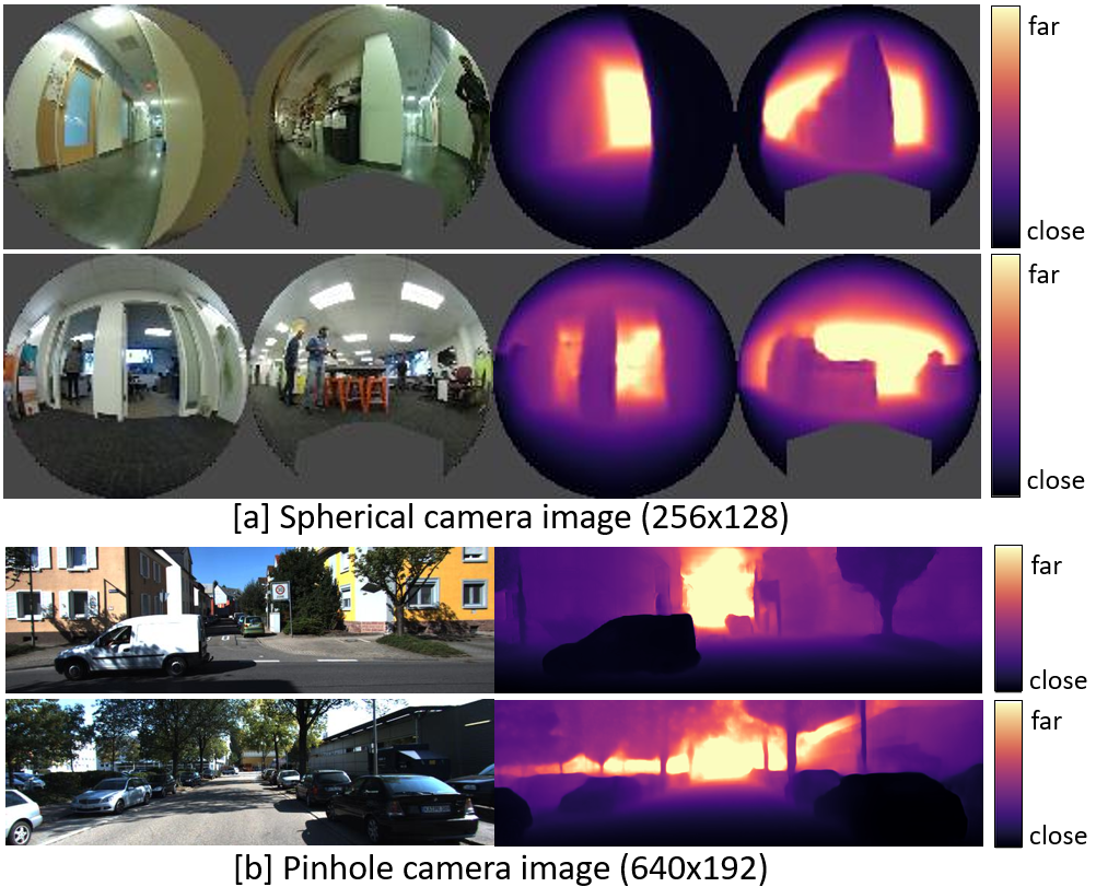
Our method was trained and evaluated on the GO Stanford (GS) dataset [9, 10, 11], as depicted in in Fig 1[a], with time-sequence spherical camera images and associated reference velocities for dataset collection. Moreover, we solely evaluated the most important contribution, that is, the learnable axisymmetric camera model on the common KITTI dataset [12], as depicted in Fig 1[b], to provide a comparison with other learnable camera models [13, 14]. We quantitatively and qualitatively evaluated our method with the GS and KITTI datasets.
II RELATED WORK
Monocular depth estimation using self-supervised learning has been widely investigated by several approaches that use deep learning [15, 16, 17, 6, 18, 19, 20, 4, 13, 21, 22]. Zhou et al. [3], and Vijayanarasimhan et al. [23] applied spatial transformer modules [24] based on the knowledge of structure from motion to achieve self-supervised learning from time-sequence images. Since the publication of [3] and [23], several subsequent studies have attempted to estimate accurate depth using different methods, including a modified loss function [25], an additional loss function to penalize geometric inconsistencies [5, 26, 13, 27, 7], a probabilistic approach to estimate the reliability of depth estimation [22, 28], masking dynamic objects [4, 13], and an entirely novel model structure [17, 29, 30]. We review the two categories most related to our method.
Fisheye camera image. Various approaches have attempted to estimate depth images from fisheye images. [31] proposed supervised learning with sparse GT from LiDAR. [32, 33, 34] leveraged multiple fisheye cameras to estimate a 360∘ depth image. Similarly, Kumar et al. proposed self-supervised learning approaches with a calibrated fisheye camera model [35] and semantic segmentation [36].
Learning camera model. Gordon et al. [13] proposed a self-supervised monocular depth estimation method that can learn the camera’s intrinsic parameters. Vasiljevic et al. [14] proposed a learnable neural ray surface (NRS) camera model for highly distorted images.
In contrast to the most related work [14], our learnable axisymmetric camera model is fully differentiable without the softmax approximation. Hence, end-to-end learning can be achieved without adjusting the hyperparameters during training. In addition, we provide supervision for the estimated depth images by using a photo-realistic simulator and robot trajectories from the dataset. As a result, our method can accurately estimate the depth from low-resolution spherical images.
III PROPOSED METHOD
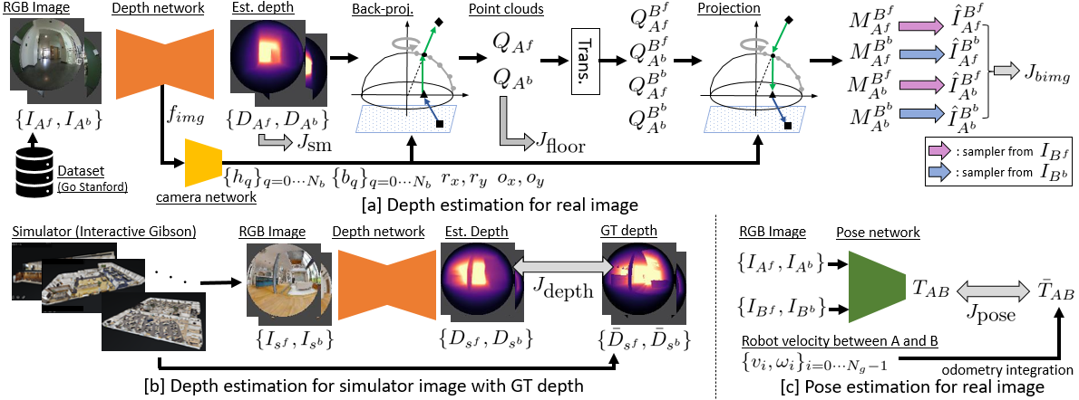
From the process in Fig. 2, we designed the following cost functions to train the depth, pose and camera networks:
| (1) |
In , we propose a learnable camera model to handle the image sequences with unknown camera parameters. Our camera model can be trained without the GT camera parameters, through minimization of for self-supervised monocular depth estimation. The camera model has the learnable convex projection surface to deal with the arbitrary distortion, e.g. spherical camera image with two fisheye images. Contrary to the image loss of baseline methods [3, 25], is an occlusion-aware image loss using our learnable camera model to leverage the advantage of the 360∘ view around the robot by the spherical camera.
penalizes the depth difference using the GT depth from photo-realistic simulator. By penalizing with , our model can learn sim2real transfer and can thereby estimate accurate depths from real images. is the proposed loss function that provides supervision against floor areas by using robot’s footprint and trajectory.
In addition to these major contributions, penalizes the difference between the estimated pose and the GT pose calculated from the reference velocities in the dataset. penalizes the discontinuity of the estimated depth using the exactly same objective, following [16, 25].
In the following sections, we first present and in the overview of the training process. Then, we explain our camera model as the main contribution. Finally, we introduce and to improve the performance of depth estimation.
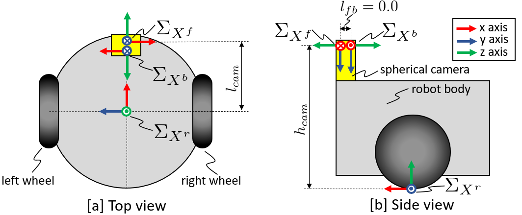
We define the robot and camera coordinates based on the global robot pose , as shown in Fig. 3. is the base coordinate of the robot. In addition, and are the camera coordinates of the front- and back-side fisheye cameras in the spherical camera, respectively. The axes directions are shown in Fig. 3. Following convention of the camera coordinate, we define the axis as downward and the axis as forward in and . Additionally, and are opposite around axis on their coordinates. We assume that the relative poses between each coordinate are known after measuring the height and the offset of the camera position.
III-A Overview
III-A1 Process of depth estimation
Fig. 2[a] presents the calculation of depth estimation for real images. Since there are no GT depth images, we employed self-supervised learning approach using time-sequence images. Unlike previous approaches[3, 25], our spherical camera can capture both the front- and back-side of the robot. Hence, we propose a cost function to blend the front- and back-side images and thereby reduce the negative effects of occlusion.
We feed the front-side images and back-side image at robot pose into the depth network to estimate the corresponding depth images as . By back-projection with our proposed camera model, we can obtain the corresponding point clouds and for each camera coordinate and , respectively.
| (2) |
Opposed to the baseline methods, our method predicts both the front- and back-side images from a single side image to blend them in . Hence, “Trans.” in Fig. 1[a] transforms the coordinates of the estimated point clouds as follows:
| (3) | |||
Here, denotes the point clouds on the coordinate estimated from image . is the estimated transformation matrix between and . is the known transformation matrix between and . By projecting these point clouds with our learnable camera model, we can estimate four matrices ,
| (4) |
where, and . According to [24], we estimate by sampling the pixel value of as . Here denotes the estimated image of by sampling . Note that we estimated four images from the combination of and , as shown in Fig. 2[a]. We calculate the blended image loss to penalize the model during training.
| (5) | |||
Here, selects a smaller value at each pixel and calculates the mean of all the pixels. is the pixel-wise structural similarity (SSIM) [37], following [25]. By selecting a smaller value in , we can equivalently select the non-occluded pixel value of or to calculate L1 and SSIM [25]. is a mask to remove the pixels without RGB values and those of the robot itself, which are depicted in gray color in Fig. 1[a].
III-A2 Process of pose estimation
Fig. 2[c] denotes the process to estimate . Unlike previous monocular depth estimation approaches, we use the GT transformation matrix from the integral of the reference velocities to move between poses and . is designed as .
III-B Learnable axisymmetric camera model
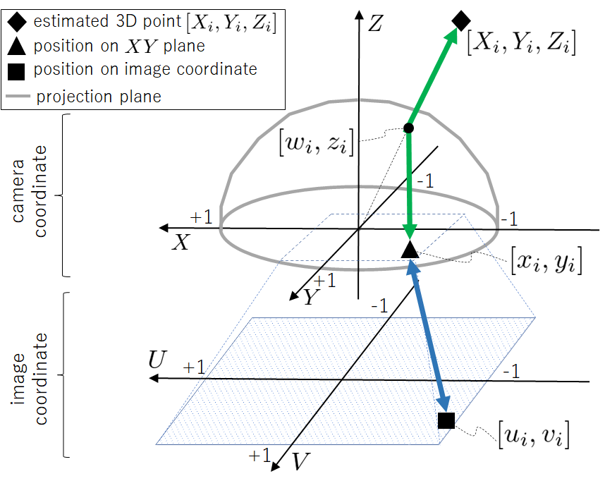
Our camera model defines the relationship between the pixel position on the image coordinates and corresponding 3D point on the camera coordinates. This mapping has been written as or during the training process. Since we formulate a differentiable model, all parameters in our model can be simultaneously trained along with depth and pose networks.
Figure 4 shows an overview of the camera model. There are two individual processes: 1) (blue double arrow) for modeling the field of view (FoV) and the offset similar to the camera intrinsic parameters, and 2) (green double arrow) for handling the camera distortion. These processes are connected at on plane of the camera coordinate. We explain each of the separate processes in the following paragraphs. To accept arbitrarily sized images, the image coordinate is regularized within [-1, 1] and origin is positioned at the center of the image.
III-B1 Part I
The mapping between and is defined by four independent parameters: for the FoV, and for the offset between and . Assuming linear relationships, this part of is written as follows,
| (6) |
where . Owing to the linearity and regularity, defining the inverse transformation for as is straightforward.
III-B2 Part II
Next, we show the process of the green double arrow between and in Fig. 4 to model the distortion. At first, we design the learnable projection surface (grey color lines in Fig. 4). Then, we explain the computation procedure in and .
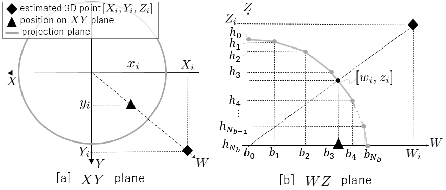
Projection surface
Figure 5 indicates the details of our projection surface, which is axisymmetric around the axis and convex upwards. Unlike the baseline camera model [38, 39], our projection surface is modeled as a linear interpolation of a discrete surface to effectively train the camera model in self-supervised learning, inspired by Bhat et al. [40]. Note that Bhat et al. [40] discritizes the estimated depth itself and interpolates them in supervised learning architecture for explicit depth estimation, unlike our approach.
This projection surface can define a unique mapping between the angle of incident light and radial position of projected point on the plane, which reflects the distortion property of the camera. The projection surface on the plane is defined as consecutive line segments by the points in Fig. 5[b]. Here, the axis is defined as the radial direction from the origin towards as shown in Fig. 5[a]. Because the parameters are normalized to stabilize the training process, the projection surface on the plane can be depicted as a unit circle centered at the origin, as shown in Fig. 5[a]. By giving the constraint and , the convex upwards shape can be ensured. This constraint is indispensable to be fully differentiable model, as shown in b) Back-projection and c) Projection. Here , . indicates the variable before applying normalization.
Our camera network estimates all parameters in our camera model as follows:
| (7) |
where is the image features from the depth encoder. In , we provide a sigmoid function at the last layer to achieve and . By simple algebra with and , we can obtain . By performing normalization to stabilize the training process, we can obtain and .
Back-projection
To calculate from the estimated depth at , we first calculate , which is the intersection point on the projection surface. The line of the -th line segment of the projection surface on the plane can be expressed as:
| (8) |
To achieve a fully differentiable process, we calculate the intersection points between all lines of the projection surface and the vertical line . Then, we select the minimum height at all intersections as because the projection surface is upwardly convex.
| (9) |
Here, the min function is a differentiable function. Note that searching the corresponding line segment by element-wise comparison instead of the above calculation is not differentiable. Based on , we can obtain and .
Projection
Similarly to back-projection, we first calculate the intersection point and derive from . The line between the origin and can be expressed as . Much like the back-projection process, the minimum value at all intersections on the axis can be . Hence, and can be derived as follows:
| (10) |
Thus, . Here, .
In both back-projection and projection, we clamp between and , and do not consider the points outside the unit circle on the plane as the out of view points.
III-C Floor loss
The highly reflective floor surface in indoor environments can often cause significant artifacts in depth estimation. Our floor loss function provides geometric supervision for floor areas. Assuming that the camera is horizontally mounted on the robot and its height is known, the floor loss function is constructed by two components: .
III-C1 Footprint consistency loss
The robot footprint is almost horizontally flat, and its height is obtained from the camera mounting position. According to the method shown below, we obtain the GT depth only around the robot footprint between steps and provide the supervision as follows:
| (11) |
where is the mask, which masks out the pixels without the GT values in , and is the number of pixel with the GT depth. can be derived as:
| (12) |
where and are the values of the axis of . Here, is the point clouds of the robot footprint between steps on . To obtain , we calculate the robot local positions using the teleoperator’s velocity between steps. And, is the known transformation matrix from to . By assigning all point clouds into using (12), we can take to calculate . Note that is a sparse matrix. No GT pixel in is excluded by .
III-C2 lower boundary loss
In indoor scenes, floor areas often reflect ceiling lights. This can cause it to appear that there are holes on the floor in the estimated depth image. To provide a lower boundary for the height of estimated point clouds, we observe two key points: 1) the camera is horizontally mounted on the robot, and 2) most objects around the robot are higher than the floor. One exception would be anything that is downstairs, which would be lower than the floor. However, it is rare in to find such occurrences in the dataset, because teleoperation around the stairs is dangerous and ill-advised.
To provide the constraint for the axis ( hight) value of the estimated point clouds, can be given as follows:
| (13) |
where . penalizes , which is larger ( lower) than the floor height ().
III-D Sim2real transfer with
In conjunction with self-supervised learning using time-sequence real images, we used the GT depth image from a photo-realistic robot simulator [41, 42], as shown in Fig. 2[b]. Although there is an appearance gap between real and simulated images, the GT depth from the simulator can help the model understand the 3D geometry of the environment from the image. Here, , where . and are front- and back-side fisheye images, respectively, from the simulator. We employed the same metric as the baseline method [43] to measure the depth differences. To achieve a sim2real transfer, we simultaneously penalized and .
IV EXPERIMENT
IV-A Dataset
Our method was mainly evaluated using the GO Stanford (GS) dataset with time-sequence spherical camera images. In addition, we used the KITTI dataset with pinhole camera images for comparison with the baseline methods, which attempts to learn the camera parameters.
IV-A1 GO Stanford dataset
We used the GS dataset [9, 10, 11] with time-sequence spherical camera images (256128) and the reference velocities, which were collected by teleoperating turtlebot2 with Ricoh THETA S. The GS dataset contains 10.3 hours of data from twelve buildings at the Stanford University campus. To train our networks, we used a training dataset from eight buildings, following [11].
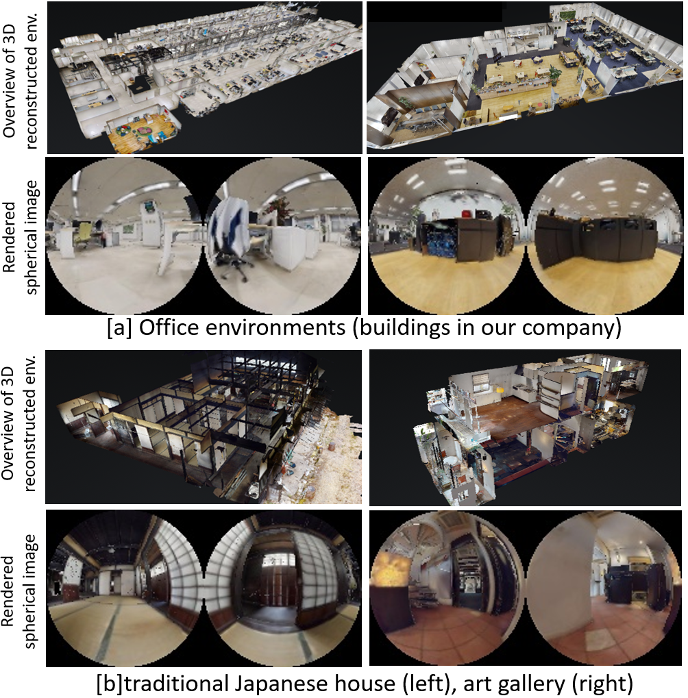
In addition to the real images of the GS dataset, we collected pairs of simulator images and GT depth images for . We scanned 12 floors (e.g., office rooms, meeting rooms, laboratories) in our company buildings and ten environments (e.g., a traditional Japanese house, art gallery, fitness gym) for the simulator by Matterport pro2, as shown in Fig. 6. We separated them into groups: eight floors in our company buildings for training, four floors in our company buildings for validation, and ten environments not in our company for testing. For training, we rendered 10,000 data from each environment using interactive Gibson [41, 42]. In addition, we collected 1,000 data points for testing from ten environments.
Data collection of the GT depth from a real spherical image is a challenging task. Hence, in the quantitative analysis, we used the GT depth from the simulator. To evaluate the generalization performance, our test environment was not derived from our company building. Examples of the domain gaps between training and testing are shown in Fig. 6. In the qualitative analysis, we used both real and simulated images.
| Method | SGT | Abs-Rel | Sq-Rel | RMSE | |
|---|---|---|---|---|---|
| monodepth2 [25] | 0.586 | 1.890 | 1.123 | 0.439 | |
| –with SGT[25, 43] | ✓ | 0.228 | 0.162 | 0.535 | 0.664 |
| Alhashim et al. [43] | ✓ | 0.203 | 0.154 | 0.542 | 0.698 |
| \hdashlineOur method (full) | ✓ | 0.198 | 0.143 | 0.525 | 0.711 |
| –wo | 0.377 | 0.335 | 0.829 | 0.433 | |
| –wo our cam. model | ✓ | 0.248 | 0.179 | 0.548 | 0.646 |
| –wo | ✓ | 0.233 | 0.161 | 0.532 | 0.665 |
| –wo | ✓ | 0.216 | 0.151 | 0.530 | 0.684 |
| –wo blending in | ✓ | 0.205 | 0.147 | 0.530 | 0.702 |
| –wo | ✓ | 0.200 | 0.145 | 0.532 | 0.698 |
| Method | Camera | Abs-Rel | Sq-Rel | RMSE | |
|---|---|---|---|---|---|
| Gordon et al. [13] | known | 0.129 | 0.982 | 5.23 | 0.840 |
| Gordon et al. [13] | learned | 0.128 | 0.959 | 5.23 | 0.845 |
| \hdashlineNRS [44] | known | 0.137 | 0.987 | 5.337 | 0.830 |
| NRS [44] | learned | 0.134 | 0.952 | 5.264 | 0.832 |
| \hdashlinemonodepth2 (original) | known | 0.115 | 0.903 | 4.864 | 0.877 |
| with our cam. model | known | 0.115 | 0.915 | 4.848 | 0.878 |
| with our cam. model | learned | 0.113 | 0.885 | 4.829 | 0.878 |
| with our cam. model | learned | 0.109 | 0.826 | 4.702 | 0.884 |
IV-A2 KITTI dataset
To evaluate our proposed camera model against the baseline methods, we employed the KITTI raw dataset [12] for the evaluation of depth estimation. Similar to the baseline methods, we separated the KITTI raw dataset via Eigen split [45] with 40,000 images for training, 4,000 images for validation, and 697 images for testing. To compare with baseline methods, we employed the widely used 640192 image size as input.
Besides, we used the KITTI odometry dataset with ground truth pose for the evaluation of pose estimation. It is known that the KITTI raw dataset for depth estimation partially includes test images from the KITTI odometry dataset. Hence, following the baseline methods, we trained our models with sequences 00 to 08 and conduct testing on sequences 09 and 10.
IV-B Training
In training with the GS dataset, we randomly selected 12 real images from the training dataset as . Then, we randomly selected between 5(= ) steps. In addition, we selected 12 simulator images and the GT depth for .
To define the transformation matrices , , and , we measured and in Fig. 3 as 0.57 and 0.12 meters, respectively. Additionally, we set for our camera model. The weighting factors for the loss function were designed as , , , , and . , , and were exactly the same as in previous studies. We only determined by trial and error.
The robot footprint shape was defined as a circle with a diameter of 0.5 m. The point cloud of the footprint was set as 1400 points inside the circle. The number of steps for the robot footprints was for .
The network structures of and were exactly the same as those of monodepth2 [25]. In addition, was designed with three convolutional layers, with the ReLu function and two fully connected layers with a sigmoid function, to estimate the camera parameters. We used the Adam optimizer with a learning rate of 0.0001 and conducted training loop for 40 epochs.
During training, we iteratively calculated and derived the gradient to update all the models. Hence, we could simultaneously penalize from the simulator and the others from the real images to achieve a sim2real transfer.
For the KITTI dataset, we employed the source code of monodepth2 [25] and replaced the camera model with our proposed camera model. The other settings were exactly the same as those of monodepth2, to focus the experimentation on our camera model.
IV-C Evaluation of depth estimation
IV-C1 Quantitative Analysis
Table I shows the ablation study of our method and the results of three baseline methods for comparison. We trained the following baseline methods with the same dataset.
monodepth2 [25] We applied the following half-sphere model [46] into monodepth2 [25], instead of the pinhole camera model, and trained depth and pose networks. This model assumes that the coordinate is the same as the coordinate and the projection surface is a half-sphere.
back-projection: (, , ) (, ),
| (14) |
Projection: (, , ) (, )
| (15) |
monodepth2 with sim. GT [25, 43] We added to the cost function of the above baseline to train the models.
Alhashim et al. [43] We trained the depth network by minimizing , which is the same cost function as [43].
In quantitative analysis, we evaluate the estimated depth using common metrics. “Abs-Rel,” “Sq-Rel,” and “RMSE,” are calculated by means of the following values.
-
•
Abs-Rel :
-
•
Sq Rel :
-
•
RMSE :
Here, is the ground truth of the estimated depth image . The remaining metric is the ratios that satisfy . is defined as .
From Table I, we can observe that our method significantly outperforms all baseline methods. In addition, we confirmed the advantages of our proposed components via the ablation study. The use of the GT depth from the simulator and the learning axisymmetric camera model were fairly effective. Even though the proposed method is evaluated without scaling using the GT depth, it outperforms the other methods with scaling. This suggests that our method learns the correct scaling via with the GT depth from the simulator.
In Table II, we present the quantitative results for the KITTI dataset. Similar to our method, the baseline methods (shown in Table II) learned the camera model. All methods presented in Table II used ResNet-18 for their depth network to allow for fair comparisons.
In our method with known camera parameters, we set , , , , and as the constant values for the GT camera’s intrinsic parameters. was designed with equal intervals between 0.0 and 1.0. Our method improved the accuracy of depth estimation by learning the camera model. In addition, our method outperformed all baseline methods, including the original monodepth2.
Moreover, we trained our models by mixing the KITTI, Cityscape [47], bike [5], and GS datasets [11] to evaluate its ability to handle various cameras and evaluated on KITTI images. During training, all images were aligned into KITTI’s image size by center cropping. In GS dataset, we use front-side fisheye images. Our method showed improved performance by adding datasets from various cameras with various distortions, as shown at the bottom of Table II.
IV-C2 Qualitative Analysis
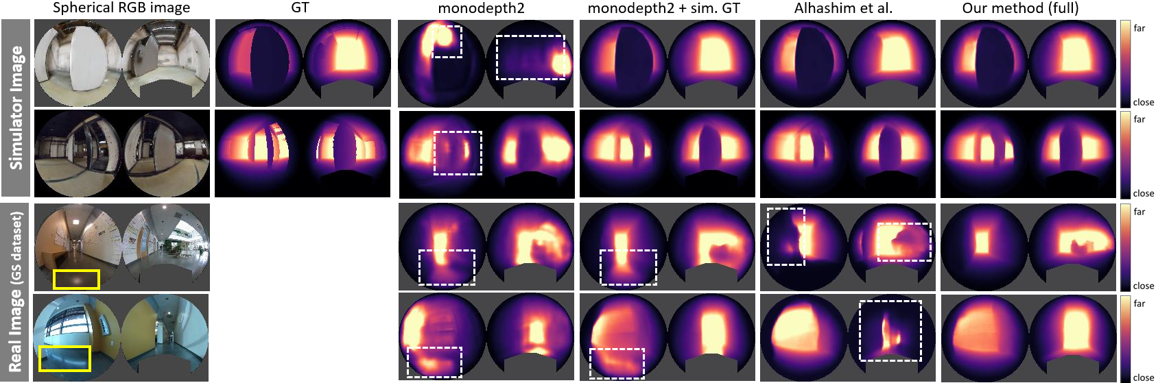
Figure 7 shows the estimated depth images from simulated images and real images from the GS dataset. The depth images estimated by monodepth2 are blurred. This is caused by the small size of the input image and the camera model’s error. The GT depth from the simulator can sharpen the simulated depth of images in monodepth2 with sim. GT. However, there are many artifacts, particularly on the reflected floor. Alhashim et al. observed errors in the estimated depth from real images. Alhashim et al. failed sim2real transfer because the depth network was trained only from simulated images. However, our method (rightmost side) can accurately estimate depth images of both real and simulated images by reducing these artifacts. Additional examples are provided in the supplemental videos.
Finally, we present the depth images of KITTI in Fig. 1 [b]. Our method can handle the pinhole camera image and estimate an accurate depth image without camera calibration.
IV-D Evaluation of pose estimation
We evaluate our pose network using the KITTI odometry dataset with the ground truth poses. Table III shows the mean and standard deviation of absolute trajectory error over five-snippets in the test dataset, following the baseline methods. Although Gordon et al. [13] with known camera model shows explicit advantages, their performance deteriorates while learning the camera parameters. Besides, our method with learning our camera model shows a healthy advantageous gap against the original monodepth2 with known camera intrinsic parameters.
| Method | Camera | Sequence 09 | Sequence 10 |
|---|---|---|---|
| Gordon et al. [13] | known | 0.009 0.0015 | 0.008 0.011 |
| Gordon et al. [13] | learned | 0.0120 0.0016 | 0.010 0.010 |
| \hdashlineNRS [44] | known | – | – |
| NRS [44] | learned | 0.0150 0.0301 | 0.0103 0.0073 |
| \hdashlinemonodepth2 (original) | known | 0.017 0.008 | 0.015 0.010 |
| with our cam. model | learned | 0.0134 0.0068 | 0.0134 0.0084 |
V CONCLUSIONS
We proposed a novel learnable axisymmetric camera model for self-supervised monocular depth estimation. In addition, we proposed to supervise the estimated depth using the GT depth from the photo-realistic simulator. By mixing real and simulator images during training, we can achieve a sim2real transfer in depth estimation. Additionally, we proposed loss functions to provide the constraints for the floor to reduce artifacts that may result from reflective floors. The effectiveness of our method was quantitatively and qualitatively validated using the GS and KITTI datasets.
VI ACKNOWLEDGMENT
We thank Kazutoshi Sukigara, Kota Sato, Yuichiro Matsuda, and Yasuaki Tsurumi for measuring 3D environments to collect pairs of simulator images and GT depth images.
References
- [1] S. Thrun, “Probabilistic robotics,” Communications of the ACM, vol. 45, no. 3, pp. 52–57, 2002.
- [2] J. Biswas and M. Veloso, “Depth camera based indoor mobile robot localization and navigation,” in 2012 IEEE International Conference on Robotics and Automation. IEEE, 2012, pp. 1697–1702.
- [3] T. Zhou et al., “Unsupervised learning of depth and ego-motion from video,” in Proceedings of the IEEE Conference on Computer Vision and Pattern Recognition, 2017, pp. 1851–1858.
- [4] V. Casser et al., “Depth prediction without the sensors: Leveraging structure for unsupervised learning from monocular videos,” in Proceedings of the AAAI Conference on Artificial Intelligence, vol. 33, 2019, pp. 8001–8008.
- [5] R. Mahjourian et al., “Unsupervised learning of depth and ego-motion from monocular video using 3d geometric constraints,” in Proceedings of the IEEE Conference on Computer Vision and Pattern Recognition, 2018, pp. 5667–5675.
- [6] Z. Yang et al., “Every pixel counts: Unsupervised geometry learning with holistic 3d motion understanding,” in Proceedings of the European Conference on Computer Vision (ECCV), 2018, pp. 0–0.
- [7] N. Hirose et al., “Plg-in: Pluggable geometric consistency loss with wasserstein distance in monocular depth estimation,” in 2021 International Conference on Robotics and Automation (ICRA). IEEE, 2021.
- [8] https://matterport.com, (accessed August 20, 2021).
- [9] N. Hirose et al., “Gonet: A semi-supervised deep learning approach for traversability estimation,” in 2018 IEEE/RSJ International Conference on Intelligent Robots and Systems (IROS). IEEE, 2018, pp. 3044–3051.
- [10] ——, “Vunet: Dynamic scene view synthesis for traversability estimation using an rgb camera,” IEEE Robotics and Automation Letters, vol. 4, no. 2, pp. 2062–2069, 2019.
- [11] ——, “Deep visual mpc-policy learning for navigation,” IEEE Robotics and Automation Letters, vol. 4, no. 4, pp. 3184–3191, 2019.
- [12] A. Geiger et al., “Vision meets robotics: The kitti dataset,” International Journal of Robotics Research (IJRR), 2013.
- [13] A. Gordon et al., “Depth from videos in the wild: Unsupervised monocular depth learning from unknown cameras,” in Proceedings of the IEEE International Conference on Computer Vision, 2019, pp. 8977–8986.
- [14] I. Vasiljevic et al., “Neural ray surfaces for self-supervised learning of depth and ego-motion,” in 2020 International Conference on 3D Vision (3DV). IEEE, 2020, pp. 1–11.
- [15] R. Garg et al., “Unsupervised cnn for single view depth estimation: Geometry to the rescue,” in European conference on computer vision. Springer, 2016, pp. 740–756.
- [16] C. Godard et al., “Unsupervised monocular depth estimation with left-right consistency,” in Proceedings of the IEEE Conference on Computer Vision and Pattern Recognition, 2017, pp. 270–279.
- [17] V. Guizilini et al., “Packnet-sfm: 3d packing for self-supervised monocular depth estimation,” arXiv preprint arXiv:1905.02693, vol. 5, 2019.
- [18] C. Wang et al., “Learning depth from monocular videos using direct methods,” in Proceedings of the IEEE Conference on Computer Vision and Pattern Recognition, 2018, pp. 2022–2030.
- [19] Y. Chen et al., “Self-supervised learning with geometric constraints in monocular video: Connecting flow, depth, and camera,” in Proceedings of the IEEE/CVF International Conference on Computer Vision, 2019, pp. 7063–7072.
- [20] V. R. Kumar et al., “Unrectdepthnet: Self-supervised monocular depth estimation using a generic framework for handling common camera distortion models,” arXiv preprint arXiv:2007.06676, 2020.
- [21] V. Guizilini et al., “Robust semi-supervised monocular depth estimation with reprojected distances,” in Conference on Robot Learning, 2020, pp. 503–512.
- [22] M. Poggi et al., “On the uncertainty of self-supervised monocular depth estimation,” in IEEE/CVF Conference on Computer Vision and Pattern Recognition (CVPR), 2020.
- [23] S. Vijayanarasimhan et al., “Sfm-net: Learning of structure and motion from video,” arXiv preprint arXiv:1704.07804, 2017.
- [24] M. Jaderberg et al., “Spatial transformer networks,” in Advances in neural information processing systems, 2015, pp. 2017–2025.
- [25] C. Godard and othersJ, “Digging into self-supervised monocular depth estimation,” in Proceedings of the IEEE International Conference on Computer Vision, 2019, pp. 3828–3838.
- [26] Y. Zou et al., “Df-net: Unsupervised joint learning of depth and flow using cross-task consistency,” in Proceedings of the European conference on computer vision (ECCV), 2018, pp. 36–53.
- [27] X. Luo et al., “Consistent video depth estimation,” arXiv preprint arXiv:2004.15021, 2020.
- [28] N. Hirose et al., “Variational monocular depth estimation for reliability prediction,” in 2021 International Conference on 3D Vision (3DV). IEEE, 2021, pp. 637–647.
- [29] G. Yang et al., “Transformer-based attention networks for continuous pixel-wise prediction,” arXiv preprint arXiv:2103.12091, 2021.
- [30] J. H. Lee et al., “From big to small: Multi-scale local planar guidance for monocular depth estimation,” arXiv preprint arXiv:1907.10326, 2019.
- [31] V. R. Kumar et al., “Monocular fisheye camera depth estimation using sparse lidar supervision,” in 2018 21st International Conference on Intelligent Transportation Systems (ITSC). IEEE, 2018, pp. 2853–2858.
- [32] C. Won et al., “Sweepnet: Wide-baseline omnidirectional depth estimation,” in 2019 International Conference on Robotics and Automation (ICRA). IEEE, 2019, pp. 6073–6079.
- [33] R. Komatsu et al., “360 depth estimation from multiple fisheye images with origami crown representation of icosahedron,” in 2020 IEEE/RSJ International Conference on Intelligent Robots and Systems (IROS). IEEE, 2020, pp. 10 092–10 099.
- [34] Z. Cui et al., “Real-time dense mapping for self-driving vehicles using fisheye cameras,” in 2019 International Conference on Robotics and Automation (ICRA). IEEE, 2019, pp. 6087–6093.
- [35] V. R. Kumar et al., “Fisheyedistancenet: Self-supervised scale-aware distance estimation using monocular fisheye camera for autonomous driving,” in 2020 IEEE international conference on robotics and automation (ICRA). IEEE, 2020, pp. 574–581.
- [36] ——, “Syndistnet: Self-supervised monocular fisheye camera distance estimation synergized with semantic segmentation for autonomous driving,” in Proceedings of the IEEE/CVF Winter Conference on Applications of Computer Vision, 2021, pp. 61–71.
- [37] Z. Wang et al., “Image quality assessment: from error visibility to structural similarity,” IEEE transactions on image processing, vol. 13, no. 4, pp. 600–612, 2004.
- [38] V. Usenko et al., “The double sphere camera model,” in 2018 International Conference on 3D Vision (3DV). IEEE, 2018, pp. 552–560.
- [39] J. Fang et al., “Self-supervised camera self-calibration from video,” arXiv preprint arXiv:2112.03325, 2021.
- [40] S. F. Bhat et al., “Adabins: Depth estimation using adaptive bins,” in Proceedings of the IEEE/CVF Conference on Computer Vision and Pattern Recognition, 2021, pp. 4009–4018.
- [41] F. Xia et al., “Interactive gibson benchmark: A benchmark for interactive navigation in cluttered environments,” IEEE Robotics and Automation Letters, vol. 5, no. 2, pp. 713–720, 2020.
- [42] ——, “Gibson env v2: Embodied simulation environments for interactive navigation,” Stanford University, Tech. Rep., 2019.
- [43] I. Alhashim and P. Wonka, “High quality monocular depth estimation via transfer learning,” arXiv preprint arXiv:1812.11941, 2018.
- [44] I. Vasiljevic et al., “Neural ray surfaces for self-supervised learning of depth and ego-motion,” in 2020 International Conference on 3D Vision (3DV), 2020, pp. 1–11.
- [45] D. Eigen et al., “Depth map prediction from a single image using a multi-scale deep network,” in Advances in neural information processing systems, 2014, pp. 2366–2374.
- [46] J. Courbon et al., “A generic fisheye camera model for robotic applications,” in 2007 IEEE/RSJ International Conference on Intelligent Robots and Systems. IEEE, 2007, pp. 1683–1688.
- [47] M. Cordts et al., “The cityscapes dataset for semantic urban scene understanding,” in Proc. of the IEEE Conference on Computer Vision and Pattern Recognition (CVPR), 2016.