DESI Emission Line Galaxies:
Unveiling the Diversity of [OII] Profiles and its Links to Star Formation and Morphology
Abstract
We study the [OII] profiles of emission line galaxies (ELGs) from the Early Data Release of the Dark Energy Spectroscopic Instrument (DESI). To this end, we decompose and classify the shape of [OII] profiles with the first two eigenspectra derived from Principal Component Analysis. Our results show that DESI ELGs have diverse line profiles which can be categorized into three main types: (1) narrow lines with a median width of km/s, (2) broad lines with a median width of km/s, and (3) two-redshift systems with a median velocity separation of km/s, i.e., double-peak galaxies. To investigate the connections between the line profiles and galaxy properties, we utilize the information from the COSMOS dataset and compare the properties of ELGs, including star-formation rate (SFR) and galaxy morphology, with the average properties of reference star-forming galaxies with similar stellar mass, sizes, and redshifts. Our findings show that on average, DESI ELGs have higher SFR and more asymmetrical/disturbed morphology than the reference galaxies. Moreover, we uncover a relationship between the line profiles, the excess SFR and the excess asymmetry parameter, showing that DESI ELGs with broader [OII] line profiles have more disturbed morphology and higher SFR than the reference star-forming galaxies. Finally, we discuss possible physical mechanisms giving rise to the observed relationship and the implications of our findings on the galaxy clustering measurements, including the halo occupation distribution modeling of DESI ELGs and the observed excess velocity dispersion of the satellite ELGs.
1 Introduction
Galaxies that produce strong emission lines from the HII star-forming regions, i.e. emission line galaxies (ELGs), have become one of the key observational targets for large cosmological surveys. Via the strong emission line features, one can detect and measure the redshifts of ELGs across a wide range of cosmic time with accessible observational resources and use those galaxies as tracers of the 3D large-scale structure of the Universe. Previous cosmological surveys, including the WiggleZ Dark Energy Survey (Drinkwater et al., 2010) and the Extended Baryon Oscillation Spectroscopic Survey in the Sloan Digital Sky Survey-IV (SDSS-IV eBOSS, Dawson et al., 2016) projects, have demonstrated that cosmological parameters, such as the expansion rate of the Universe and the dark energy equation of state, can be constrained via the baryonic acoustic oscillations (BAOs) (e.g., Eisenstein et al., 2005) signals detected from the ELG clustering measurements (e.g., Blake et al., 2011; Raichoor et al., 2021). The success of these programs has motivated the ongoing and upcoming surveys, including the Dark Energy Spectroscopic Instrument (DESI, Levi et al., 2013; DESI Collaboration et al., 2016a, b, 2022), the Prime-Focus Spectrograph (PFS, Takada et al., 2014), and Euclid (Euclid Collaboration et al., 2022) to select ELGs as one of the main targets and collect tens of millions of spectroscopic measurements of ELGs for their cosmological programs.
Among the emission lines produced by HII regions, the [O II] doublet has been considered as one of the key transitions for ground-based spectroscopic measurements (e.g., Comparat et al., 2015) owing to its detectibility in optical and near-infrared wavelengths from the local Universe to redshift , the cosmic epoch at the peak of the star-formation rate density (see Madau & Dickinson, 2014, for a review). The [O II] doublet can be used to not only pinpoint the redshifts of galaxies but also obtain information of galaxy physical properties, including star-formation rate (line luminosity), electron density (doublet line ratio), and gas kinematics (line width) (e.g., Kennicutt, 1998; Moustakas et al., 2006; Osterbrock & Ferland, 2006; Kassin et al., 2012; Kewley et al., 2019). However, to extract such information from spectra requires a spectral resolution, , to resolve the [O II] doublet feature (Comparat et al., 2013). This limits the exploration and characterization of the [OII] line properties of ELGs with the spectra from previous cosmological surveys, such as WiggleZ (, Drinkwater et al., 2010) and SDSS-IV eBOSS (, Dawson et al., 2016). On the other hand, the DESI survey has the required spectral resolution (DESI Collaboration et al., 2022) and will compile a large ELG catalog with resolved [OII] lines from redshift 0.6 to redshift 1.6, a redshift region rarely probed to date. With this large spectroscopic dataset, it is crucial to understand the underlying galaxy population selected as ELGs in the DESI survey and characterize their physical properties to fully utilize this big dataset and maximize the scientific returns for cosmology and galaxy science.
In this work, we explore diversity in the DESI ELG galaxy population based on their [OII] emission line profiles and investigate the relationships between the line profiles and the physical properties of the galaxies. To this end, we make use of a principal component analysis (PCA, Jolliffe, 2002, for a review), a dimensional reduction technique, to obtain the key eigen-spectra, which carry physical information of the line profiles. We use them to describe line profiles and classify galaxies. We then obtain the physical properties, such as stellar mass (), star-formation rate (SFR), and morphology parameters, of a subset of ELGs in the COSMOS field (Scoville et al., 2007) and examine the connections between line profiles and galaxy properties. This enables us to reveal possible underlying mechanisms driving the [OII] line profiles.
The structure of the paper is as follows. The datasets used in this analysis are described in Section 2. We present the PCA results in Section 3 and explore the relations between line profiles and galaxy properties in Section 4. We discuss our results and their implications in Section 5, and summarize in Section 6. Throughout the paper, we adopt a flat CDM cosmology with and (WMAP9 Hinshaw et al., 2013). We use AB magnitudes corrected with Galactic extinction (Schlegel et al., 1998).
2 Datasets
2.1 DESI ELG spectra
The Dark Energy Spectroscopic Instrument (DESI) survey (DESI Collaboration et al., 2022) is a Stage-IV project, primarily designed for probing the cosmological parameters of the Universe (Levi et al., 2013; DESI Collaboration et al., 2016a, 2024a). DESI consists of bright-time and dark-time science targets (Cooper et al., 2023; Hahn et al., 2023; Zhou et al., 2023; Raichoor et al., 2023; Chaussidon et al., 2023) with [OII] emission line galaxies (ELGs, Raichoor et al., 2023) being one of the key targets in the program. In order to obtain the desired redshift range of DESI ELGs, a specific target selection scheme is developed for the sources detected in the DESI Legacy Imaging Surveys (Dey et al., 2019), which include , , bands and near-infrared images from WISE satellite (Wright et al., 2010), via the Tractor algorithm (Lang et al., 2016) with large galaxies masked (Moustakas et al., 2023). To ensure the efficiency of DESI operations, dedicated pipelines are developed for target selection (Myers et al., 2023), survey operations (Schlafly et al., 2023) and fiber assignment (Raichoor et al., 2024).
Spectroscopic data is collected by the DESI instrumentation installed on the 4-meter Mayall Telescope at Kitt Peak National Observatory (DESI Collaboration et al., 2022; Silber et al., 2023; Miller et al., 2023). The instrument has a 3.2 degree diameter field of view covered with 5020 robotic fiber positioners. The wavelength coverage ranges from 3600 to 9800 with spectral resolution from in the shortest wavelength to in the longest wavelength. The raw spectra are processed, reduced and calibrated by an automatic pipeline (Guy et al., 2023). The redshifts of sources are then obtained via an algorithm, called (Bailey et al., 2023) (See also Brodzeller et al., 2023; Anand et al., 2024), with the redshift accuracy and precision for all types of extragalactic sources, including ELGs, being tested and validated against redshifts obtained from spectra with long exposure times and confirmed via visual inspection (Lan et al., 2023; Alexander et al., 2023).
In this analysis, we make use of the DESI spectra of ELGs observed during the Survey Validation phase (DESI Collaboration et al., 2024a) to explore the [O II] emission line profiles. The DESI SV campaign consists of two key phases, the SV1 and the one-percent survey. The SV1 observations include targets selected from a wider parameter space in order to test and finalize the target selection scheme of the DESI main survey. The one-percent survey then adopted the finalized target selection scheme and obtained the observations that cover sky area , about of the DESI final footprint (DESI Collaboration et al., 2024a).
We focus on the ELGs observed in the one-percent survey to inform the properties of ELGs of the DESI main survey. The ELGs are selected within a color-magnitude space defined with , colors, g-band magnitude and g-band fiber magnitude for preferentially including star-forming galaxies at (Raichoor et al., 2023).
We first make use of the data from the Early Data Release (DESI Collaboration et al., 2024b) which includes spectra of ELGs with robust redshift measurements that pass the redshift quality selection for ELGs, , where is the signal to noise ratio of the [OII] emission lines measured via a double-gaussian fitting (Raichoor et al., 2023) and is the difference between the values from the second best-fit model and the first best-fit model provided by (Bailey et al., 2023). This selection yields a ELG sample with redshift purity (the fraction of ELGs with redshifts and visually inspected redshifts difference smaller than km/s) greater than (Lan et al., 2023). We further select ELGs with and with spectral types identified by as galaxies. This selection yields a sample of ELGs. In addition, using line information available at different redshifts, we remove possible active galactic nuclei (AGN) contamination. The selections remove approximately of DESI ELGs. The detailed selections are described in Appendix A. Approximately ELGs pass the above selection criteria. We note that this sample includes ELGs with LOP (Low Priority) and VLO (Very Low Priority) selections (See Raichoor et al., 2023, for details) for the main DESI survey. Approximately 78% of the sample is LOP ELGs, the fiducial ELG sample for DESI clustering measurements.
2.2 The COSMOS datasets
To explore the physical properties of DESI ELGs in the context of the whole star-forming galaxy population across redshifts, we utilize the COSMOS2020 catalog (Weaver et al., 2022) which includes approximately 1.7 million sources with photometric redshifts () and physical properties of galaxies estimated based on multi-wavelength broad-band deep imaging datasets. The COSMOS field was covered by the DESI one-percent survey. Therefore, we can compile a sample with a few thousand DESI ELGs with properties derived from deep COSMOS datasets.
Catalog selection: In the COSMOS2020 data release, there are two source catalogs, the CLASSIC catalog and the FARMER catalog, which are constructed based on the SExtractor (Bertin & Arnouts, 1996) and the Tractor (Lang et al., 2016) algorithms respectively for source detection and flux measurements. The primary difference between two methods is that in the CLASSIC catalog, the fluxes of sources are measured with the aperture photometry method while in the FARMER catalog, the fluxes of sources are measured with the forced photometric best-fit models of source light distribution. As shown in Weaver et al. (2022), for sources brighter than 24 mag in Hyper Suprime-Cam z-band, these two methods yield consistent measurements with magnitude deviation lower than 0.05 magnitude. However, the FARMER catalog only includes sources within the UltraVISTA footprint (McCracken et al., 2012), which consists of about half the amount of sources in the CLASSIC catalog with the full COSMOS field coverage. To maximize the number of the matched DESI ELGs within the COSMOS catalog, we use the measurements provided by the CLASSIC catalog.
Photometric redshifts and physical properties: The COSMOS2020 catalog also includes photometric redshifts and the estimated physical properties of galaxies, including the stellar mass () and star-formation rate (SFR), based on the LePhare (Ilbert et al., 2006) and EAZY (Brammer et al., 2008) codes. These two algorithms adopt different sets of galaxy spectral energy distribution (SED) templates and different star-formation histories. For the details, we refer the readers to Weaver et al. (2022) and Gould et al. (2023).
In this work, we adopt the photometric redshifts and galaxy properties from the EAZY algorithm. This choice is motivated by the fact that for the DESI ELGs in the COSMOS2020 footprint and with , the SFR based on the emission line luminosity (Kennicutt, 1998; Kennicutt et al., 2009) from the EAZY algorithm has a higher Spearman’s correlation coefficient () with [OII] emission line luminosity, directly measured from the DESI spectra, than the estimated SFR provided by EAZY () and LePhare () codes. More specifically, we use the best-fit , the stellar mass, and the SFR based emission line luminosity from the EAZY algorithm applied to the CLASSIC catalog. We note that the COSMOS2020 catalog provides dust-reddened luminosity. We correct the dust effect by using (Kriek & Conroy, 2013) and adopt the intrinsic luminosity and SFR relation from Kennicutt et al. (2009) for the Chabrier initial mass function (Chabrier, 2003). All the stellar mass and the SFR of galaxies used in the work are based on the above method. We emphasize that the goal of this research is to explore the relationship between [OII] line profiles and physical properties of galaxies and to compare the physical properties of DESI ELGs with the properties of the overall star-forming galaxy population at similar redshifts. Identifying the most accurate estimates of physical properties of DESI ELGs is beyond the scope of this paper.
Morphological parameters: Besides the photometric redshifts and physical properties, we make use of the non-parametric diagnostics of galaxy morphology provided by the Zurich Estimator of Structural Type catalog (ZEST, Scarlata et al., 2007; COSMOS team, 2007). The catalog includes
-
•
asymmetry (A), which quantifies the rotational symmetry of galaxy light distribution;
-
•
concentration (C), which quantifies the concentration of galaxy light distribution;
-
•
Gini coefficient (G), which quantifies the uniformity of the light distribution,
-
•
M20, which is second-order moment of the brightest pixels and
-
•
R80, which is the length of the best-fit ellipse including of total light along semi-major axis in unit of arcsec (”), reflecting the observed size of the galaxy,
(e.g., Abraham et al., 2003; Lotz et al., 2004; Conselice, 2014, for a review). These parameters are derived from Hubble Space Telescope (HST) Advanced Camera for Surveys (ACS) F814W images (Scoville et al., 2007; Koekemoer et al., 2007; Leauthaud et al., 2007) for galaxies with , a depth sufficient to include all the DESI ELGs (Raichoor et al., 2023). The F814W filter covers the rest-frame near ultraviolet to optical wavelengths of DESI ELGs. At , the filter covers from to and at , it covers from to . The average width of the point spread function for the HST ACS images is (Koekemoer et al., 2007) which corresponds to kpc at and kpc at .
Combining the information from these three catalogs111 Except of DESI ELGs within the locations of the stellar masks of the COSMOS2020 catalog, the rest of DESI ELGs in the COSMOS field have matched counterparts within radius., we produce two samples of DESI ELGs with :
-
•
DESI-COSMOS: The first one, DESI-COSMOS, is the combination between the DESI ELGs and COSMOS2020 CLASSIC catalog, which is done by cross-matching sources with 0.75” radius. This yields a sample with sources having photo-z, stellar mass, and SFR measurements.
-
•
DESI-ZEST: The second sample, DESI-ZEST, includes the morphological information from the ZEST catalog by matching the DESI-COSMOS sources with the ZEST sources with 0.75” radius. This DESI-ZEST sample is a subset of the DESI-COSMOS sample, consisting of about 2,200 galaxies.
We note that there are rare cases () that one ELG has two or more galaxies within 0.75” radius from the COSMOS2020 or the ZEST catalogs. For such cases, we adopt the properties of the most massive and brightest (in F814W filter) galaxy.
In order to compare the properties of DESI ELGs and that of the overall star-forming galaxies at the similar redshifts, we construct reference samples by selecting star-forming galaxies from the COSMOS2020 catalog that satisfy
| (1) |
This functional form is adopted from Moustakas et al. (2013) for separating star-forming and quiescent galaxies with a modification on the zero point to better include star-forming galaxies based on the adopted SFR. We refer this star-forming galaxy sample from the full COSMOS2020 catalog as COSMOS-SFG. We also cross-match this COSMOS-SFG sample with the ZEST catalog with radius to obtain a sample of approximately 100,000 star-forming galaxies with morphological parameters based on HST-ACS images. This sample is referred as COSMOS-ZEST. These samples will be used in Section 4.
3 PCA decomposition and classification
The basic of the principal component analysis (PCA Jolliffe, 2002, for a review) is to calculate the eigen-values of the correlation matrix for a given dataset and the corresponding eigen-vectors. By doing so, one can identify key eigen-vectors that carry the bulk of the variance of the dataset. Via PCA, each original data vector can be described by the sum of the mean vector and a linear combination of the eigen-vectors.
In this analysis, our data matrix consists of DESI ELG spectra around [OII] emission line region (). Via the PCA decomposition, each ELG spectrum can be described as
| (2) |
where is the th ELG spectrum, is the mean spectrum of the whole ELG spectra, is th eigen-vector (eigen-spectrum), and is the coefficient for th ELG spectrum and th eigen-spectrum. In this manner, one describes each spectrum with only a few coefficients and may explore and classify [OII] profiles based on their values. This approach has been adopted in previous studies for exploring various types of astronomical datasets, such as quasar spectra, galaxy spectra, and galaxy physical properties (e.g., Suzuki, 2006; Yip et al., 2004; Taghizadeh-Popp et al., 2012). In this work, we use the weighted PCA algorithm, which takes into account the measurement uncertainty and missing data, developed by Delchambre (2015)222We use the package at https://github.com/jakevdp/wpca developed by Jake VanderPlas..
3.1 Spectral Processing
In order to perform PCA, we shift all the ELG spectra to their rest-frame based on their redshifts and project the spectra on to a common wavelength grid with a pixel size ( km/s). This pixel size corresponds to the original pixel size of DESI spectra () in the rest-frame of a source at redshift 0.6, the lower bound of the redshift in our analysis. We estimate the continuum of each spectrum using the median value of pixels around [O II] emission lines ( and ) and subtract the estimated continuum from the spectrum. We then normalize each spectrum by the maximum value of the pixels with between and of the spectrum. By doing so, the results of PCA is more sensitive to the shape variation of the [O II] emission lines, the focus of this study, than the flux difference between spectra. Finally, we remove spectra with any bad pixels and with the median S/N of the [OII] regions between and lower than 2. The final sample includes 229,996 ELGs.
3.2 Eigen-spectra
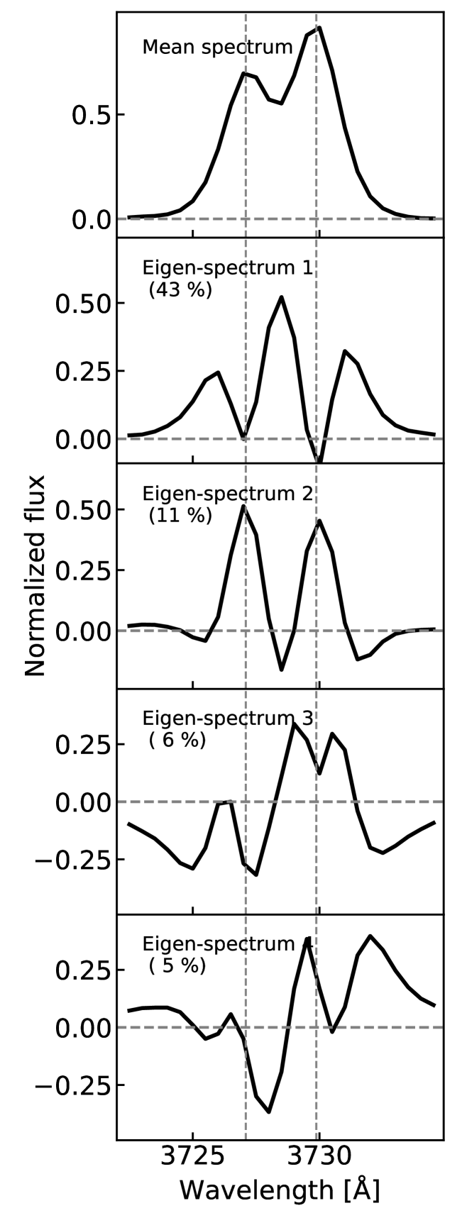
The mean spectrum and the eigen-spectra obtained by PCA are shown in Figure 1. The top panel shows the mean spectrum of the ELGs with clear [O II] emission lines. The lower four panels show the first four eigen-spectra respectively.
-
•
1st eigen-spectrum: the 1st eigen-spectrum explains of the variance of the [OII] line region. It has three peaks at 3726 , 3728.5 , and 3731 , which do not coincide with the [O II] lines. The [O II] lines in the 1st eigen-spectrum are nearly zero. By modulating flux off the line center, this eigen-spectrum broadens the line width of the emission with positive coefficients and reduces the line width with negative coefficients.
-
•
2nd eigen-spectrum: the 2nd eigen-spectrum explains of the variance. It has two peaks that coincide with the wavelengths of [O II] . With a positive value coefficient, this component increases the [O II] line strength and with a negative coefficient, it decreases the strength. Therefore, the 2nd eigen-spectrum modulates the amplitude and peakedness of the [O II] emission lines.
-
•
3rd and 4th eigen-spectra: the 3rd and 4th eigen-spectra both explain only of the variance. They both have positive values around [OII] 3730 line and negative values around [OII] 3727 line. Therefore, these two components can account for the asymmetry of the line profiles induced by both physical and non-physical signals, such as the variation of the line ratio between [OII] and [OII] (e.g., Kaasinen et al., 2017) and the residuals of sky lines.
The first two eigen-spectra explain (43%, 11%) of the total variances of the ELG spectra. In the following, we focus on the first two eigen-spectra and their application in characterizing the DESI ELG [O II] line profiles, while we plan to investigate the application of the 3rd and 4th eigen-spectra in future studies.
3.3 Coefficients
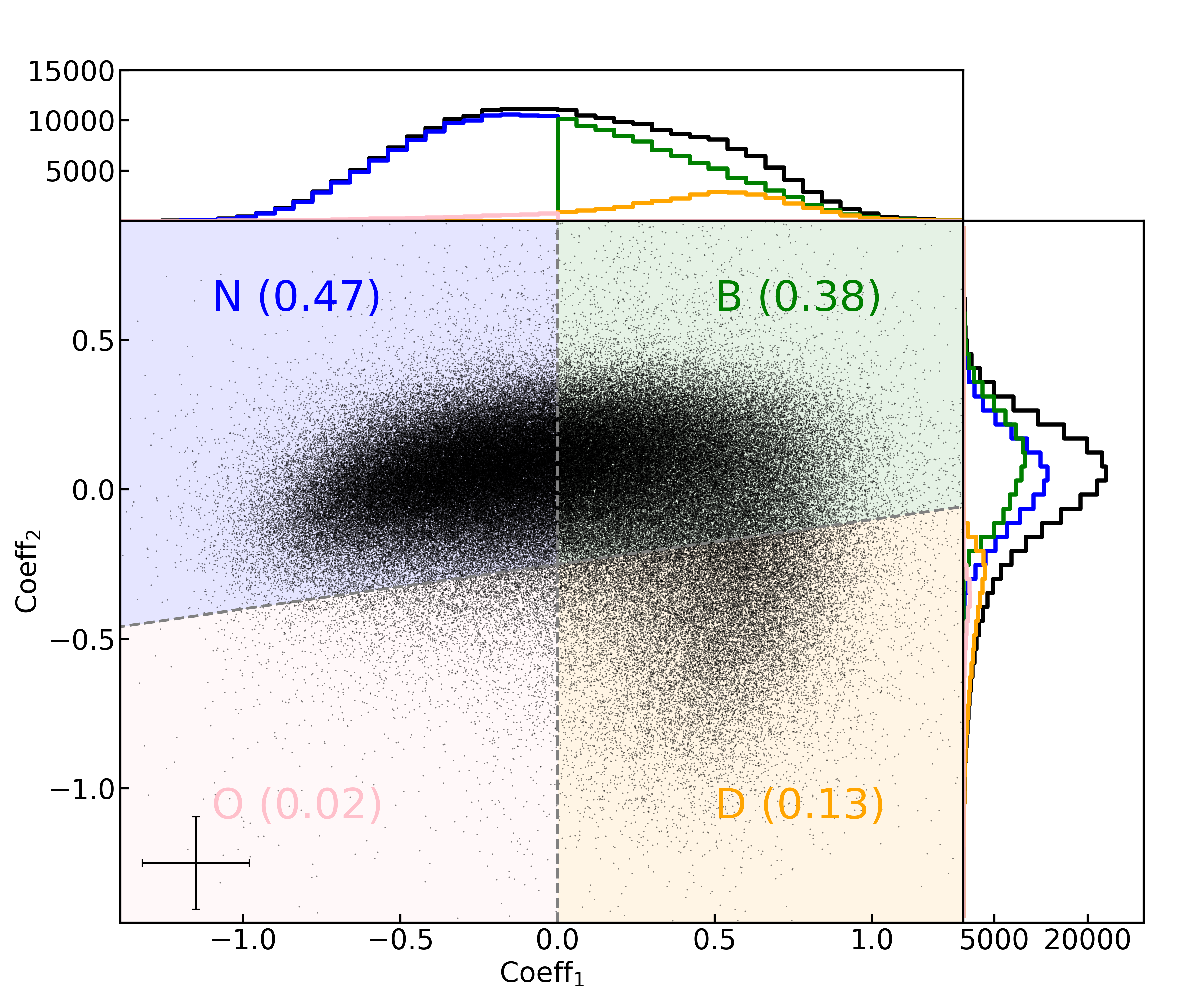
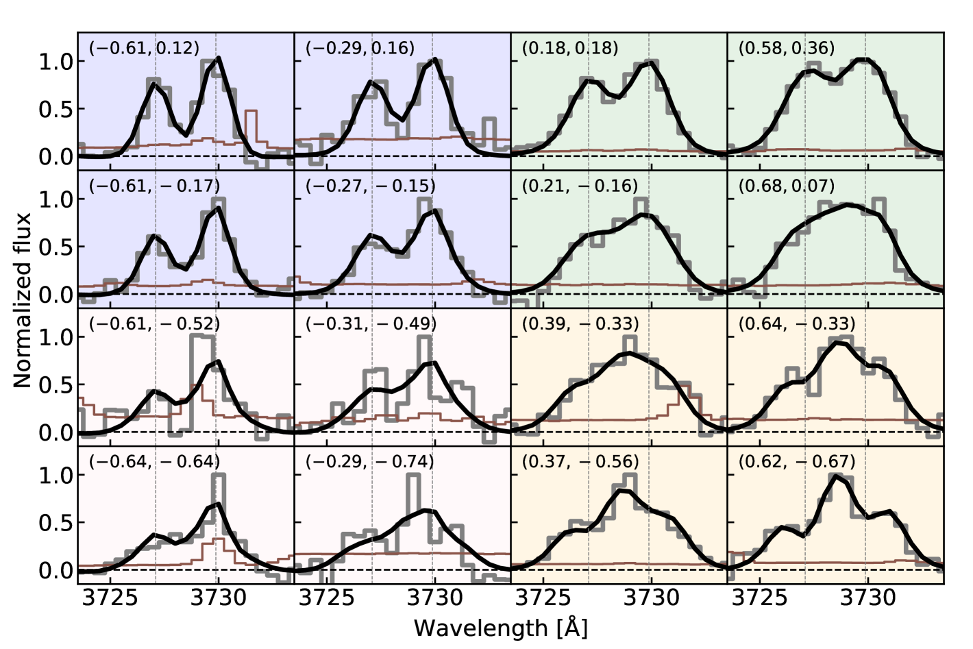
Using only the first two eigen-spectra, the [O II] line profile of each ELG can be described by two coefficients. Figure 2 shows the distribution of Coefficient 1 () (x-axis) and Coefficient 2 () (y-axis). We find that the [O II] line profiles of DESI ELGs cover the parameter space with both coefficient 1 and coefficient 2, ranging from positive to negative values. Based on the () values, we classify ELGs into four regions using two empirical selection boundaries and and show example spectra in Figure 3:
-
•
Narrow region (N): and . In this region, the doublet of [O II] is narrow and is clearly separated.
-
•
Broad region (B): and . With the increase of values, the [O II] line width becomes broader and the two [OII] lines gradually blend together with increasing .
-
•
Double-peak333 We note that the [OII] profiles have three peaks which are in fact consisted of two components with overlapping [OII] emission line doublet. For transition with a single line, the emission line profiles are double-peak. Following the literature, we use ”double-peak” galaxies for describing these systems. region (D): and . The combination of a positive value of and a negative value of yields [OII] line profiles with three emission line peaks with the central peak at as shown in lower right panels of Figure 3. These profiles are consistent with [OII] lines from two components with velocity offsets. The two velocity component spectral features are also observed in other emission lines, such as and , for low-z ELGs with double-peak emission lines. Within the selection, there are double-peak galaxies identified from the DESI EDR dataset, which is currently the largest double-peak galaxy catalog at .
-
•
Outlier region (O): and . In this region, the [OII] line profiles are affected by residuals of strong sky emission lines as shown in the lower left panels of Figure 3.
These four regions are highlighted with blue, green orange, and pink colors for narrow, broad, double-peak and outlier emission lines respectively in Figure 2. The histograms on the top and right panels show the number distributions of and respectively. We find that of ELGs are in the narrow region, of ELGs are in the broad region, are in the double-peak region, and are in the outlier region. We classify the ELGs into four regions, and emphasize that while based on the coefficients, their distribution is smooth and continuous.
3.4 Coefficients vs galaxy observed properties
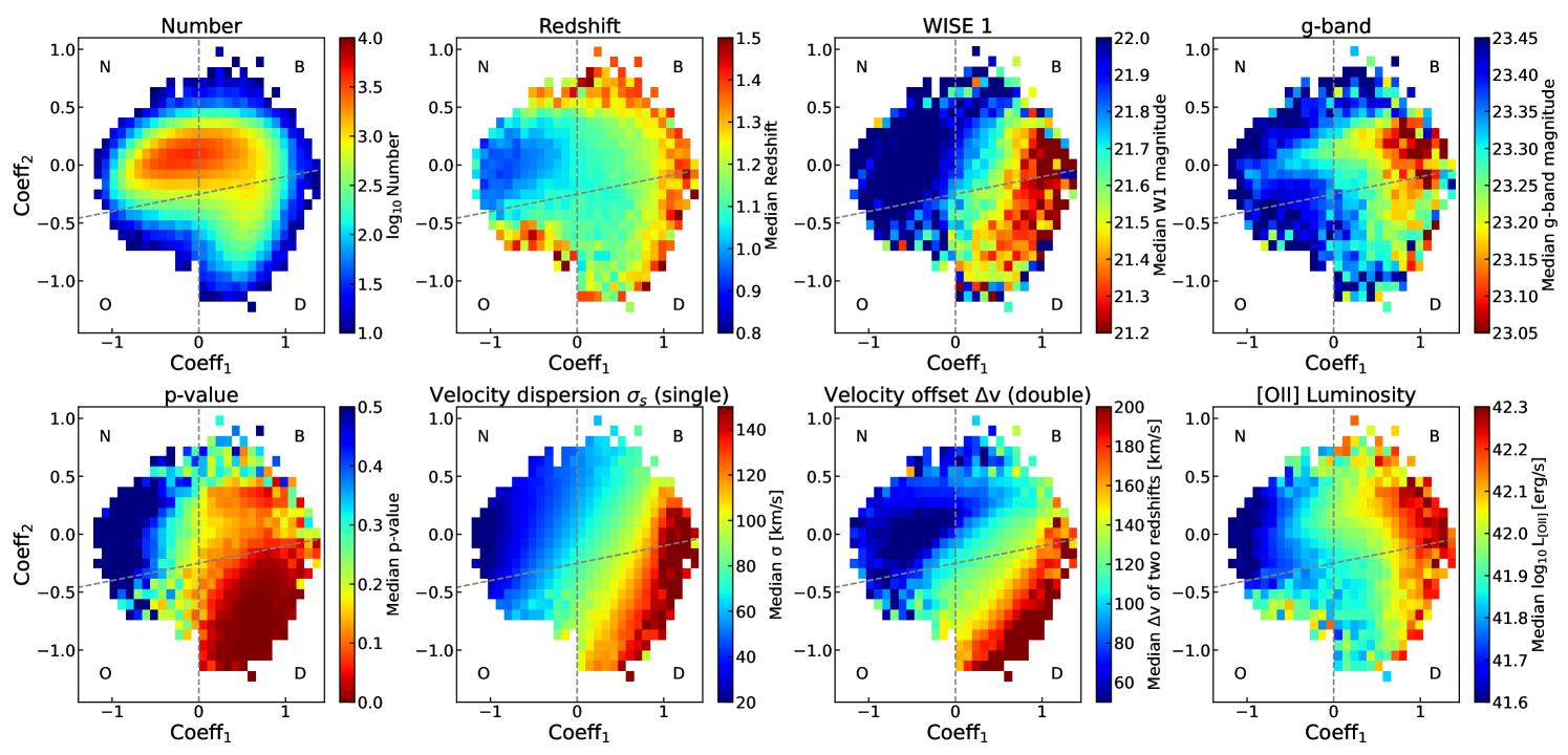
We now explore and describe the relationships between the observed properties of ELGs and values. In the upper panels of Figure 4, we first show the median values of galaxy observables in each and bin, including the number of ELGs, their redshifts, the observed WISE 1 band magnitude, and the observed g-band magnitude from left to right respectively.
Number: The first upper panel from the left shows the number distribution of DESI ELGs as a function of and . As shown in Figure 2, most of the ELGs are in the narrow and broad regions with a small fraction of ELGs in the double-peak region.
Redshifts: The second upper panel shows the median redshifts as a function of . As can be seen, there is a redshift dependence between the median redshifts and . ELGs with narrow [O II] systems () have lower median redshifts than [O II] with . Additionally, ELGs with and values near the edge of the entire distribution tend to have median redshifts . This is due to the fact that the line profiles of those galaxies are affected by sky emission line residuals and therefore have relatively extreme and values.
Observed WISE 1 band magnitude: The third upper panel of Figure 4 shows the median observed WISE 1-band magnitude of ELGs. There is a trend indicating that ELGs with larger values and lower values are on average brighter in WISE 1 band. This trend is not driven by the redshift correlation shown in the 2nd panel. It shows an opposite correlation that high-z ELGs with tend to have brighter observed magnitude than ELGs at low redshifts with . The WISE 1 band () corresponds to in the rest-frame of ELGs at , being sensitive to the stellar mass of galaxies. Therefore, the relationship between the coefficients and WISE 1 magnitude links the relationship between the coefficients and stellar mass.
Observed g-band magnitude: The last upper panel of Figure 4 shows the median g-band observed magnitude. A trend can be observed, showing the brightness of ELGs in g-band increases with the values. ELGs with on average are brighter than the rest of the ELGs. Similarly to the WISE 1 band distribution, this trend is not driven by the redshift correlation shown in the 2nd panel. We also find that the relationship between the coefficients and g-band magnitude differs from the relationship between the coefficients and WISE 1 band magnitude. DESI ELGs tend to have bright median g-band magnitude around and , while DESI ELGs tend to have bright median WISE 1-band magnitude around but extends to . Considering the g-band covers the ultraviolet wavelength in the rest-frame of ELGs, this difference suggests that the relationship between the coefficients and SFR is not entirely driven by the relationship between the coefficients and stellar mass.
In addition to the photometric properties of DESI ELGs, we extract the [OII] line information by performing spectral fitting analysis with two models. The first one, , is a single redshift model describing [O II] lines with two Gaussian profiles with a single redshift,
| (3) |
where is the wavelength (), is the amplitude of the line, is the center wavelength () of line, is line width () of the Gaussian profile. line is fitted by the second term where we adopt a fixed line ratio , the ratio between the two lines from the mean spectrum. The second model, , is a two redshift model describing [O II] lines with two sets of two Gaussian profiles, , with a wavelength offset ,
| (4) | ||||
where describes the amplitude difference in terms of ratio between the lines from two redshifts. With these two models, we obtain the best-fit parameters and the of the two models for all the ELG [O II] profiles. The lower panels of Figure 4 summarizes the fitting results.
p-value: We first quantify the performance of the two models for describing the [O II] profiles with F-test by following Maschmann et al. (2020). We estimate , where and are the values of the best-fits from the single and two redshift models and and are the corresponding degree of freedoms. We convert values into the p-value for this hypothesis test with the null hypothesis being that the model does not provide a better fit than the model. In other words, lower p-values indicate a higher probability of rejecting the null hypothesis.
The first lower panel of Figure 4 from the left shows the median p-values, indicating that the p-values depend on the and . For systems with negative values, the p-values are around 0.5, suggesting that the single redshift model is sufficient to describe the two [OII] lines. The median p-values decrease with the values. This indicates that broader line profiles tend to require two components for describing the line profiles, especially the line profiles with three emission line peaks in the double-peak region which have median p-values lower than 0.05 (a commonly adopted threshold for rejecting the null hypothesis).
Line velocity properties: The second and the third lower panels of Figure 4 show the median velocity dispersion of the emission lines estimated from the line width parameter of the single redshift model and the median velocity separation estimated from the parameter of the two redshift model respectively. We report the velocity dispersion with the spectral resolution effect being corrected. Both parameters increase from the top left corner () to the bottom right corner (). The median velocity dispersion for DESI ELGs in the narrow region, broad region, the double-peak region are km/s, km/s, and km/s respectively. For the systems that require two redshifts, velocity dispersion from the single redshift model partially reflects the velocity offset of the redshift difference shown in the third panel. The median velocity offsets for DESI ELGs in the broad and double-peak regions are km/s and km/s.
[OII] luminosity: Finally, the last lower panel of Figure 4 shows the median total luminosity (erg/s) of the two [OII] lines estimated with the best-fit of the two redshift model. There is a correlation between [OII] luminosity and , indicating that ELGs with broader line profiles have on average higher [OII] luminosity, a trend similarly to the g-band magnitude. This trend is detected across the entire redshift range probed in this work. Considering [OII] luminosity as a tracer of star-formation rate (SFR) of galaxies (e.g., Kennicutt, 1998), this result indicates that the SFR of ELGs correlates with the emission line profiles – the broader the line, the higher the SFR.
4 Relationships between line profiles and galaxy physical properties
4.1 Star-formation rate and stellar mass
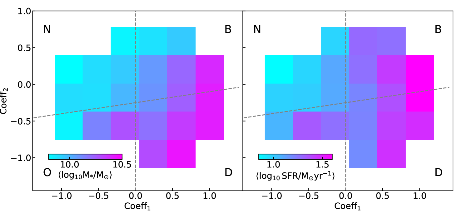
With the observed and spectral properties of DESI ELGs being explored, in order to better understand the underlying relationship, we now explore the physical properties of DESI ELGs and their connections to the [O II] line profiles, using the DESI-COSMOS sample as described in Section 2. Figure 5 shows the median values of ELG stellar mass (left panel) and SFR (right panel) in the - parameter space. The colors reflect the values of stellar mass and SFR. Being consistent with the trend observed in the median values of WISE 1 band magnitude and g-band magnitude shown in Figure 4, the stellar mass and SFR increase with , demonstrating the overall relationship between the line profiles, stellar mass and SFR.
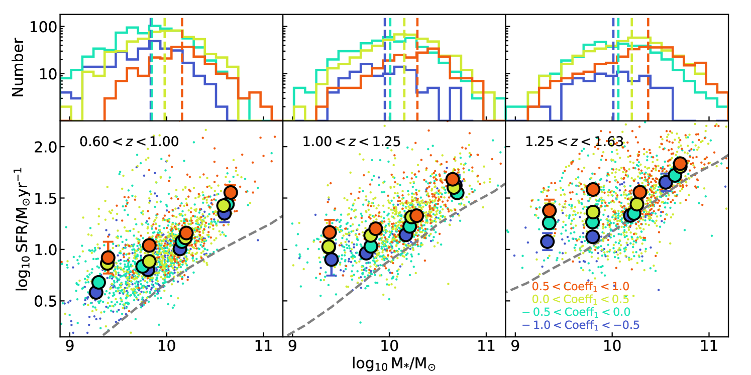
Given that the stellar mass and SFR of star-forming galaxies correlate with each other, we further investigate the correlation between and SFR with a fixed range of stellar mass of ELGs. The results are shown in Figure 6 for three redshift bins from (left), (middle), and (right). The upper panels show the stellar mass distributions of ELGs with different ranges. The vertical color dashed line shows the median stellar mass for each bin, indicating that ELGs with higher values on average have higher stellar mass.
The lower panels of Figure 6 show the SFR of ELGs as a function of stellar mass with colors indicating their values. The data points with uncertainties are the median values of for the four bins. The uncertainties are estimated by bootstrapping the sample 1000 times. We find that with a fixed stellar mass, the SFR increases with . This trend is observed across the stellar mass and redshift ranges of the DESI ELG sample. We also calculate the median SFR of the overall star-forming galaxy population at the same redshift range from the COSMOS-SFG sample defined in Sec 2.2. The grey dashed line in each panel shows the corresponding median trend. As can be seen, the majority of DESI ELGs have SFR higher than the median SFR of the overall star-forming galaxy population. This result indicates that DESI preferentially selects star-forming galaxies with SFR higher than the main sequence galaxies, a conclusion also reached by Yuan et al. (2023) using DESI ELGs with based on a similar analysis.
To summarize, Figure 6 demonstrates that while there is a general trend between the line profiles and the stellar mass and SFR which are coupled together due to the overall stellar mass and SFR correlation, there is an additional correlation between SFR and line profiles when considering ELGs with similar stellar mass. This trend is consistent with the correlation between gas velocity dispersion and SFR of star-forming galaxies observed at different redshifts from the local Universe (e.g., Law et al., 2022), (e.g., Mai et al., 2024), to (e.g., Übler et al., 2019). In the following, we explore the relationship between this excess SFR with respect to the overall star-forming galaxy population and lines profiles and investigate possible mechanisms behind this relationship.
4.2 Excess SFR, galaxy morphology, and line profiles
To explore how the excess SFR of ELGs correlates with the line profiles and inform the underlying mechanisms, in addition to the stellar mass and SFR, we use the DESI-ZEST sample which includes five morphological properties derived from HST ACS F814W images from the ZEST catalog (Scarlata et al., 2007) in the analysis: asymmetry (A), Gini coefficient (G), concentration (C), and the second-order moment of the brightest pixels (M20), and R80 parameter reflecting the galaxy size of ELGs. In Appendix B, we summarize the average relationships between line profiles and the morphological properties.
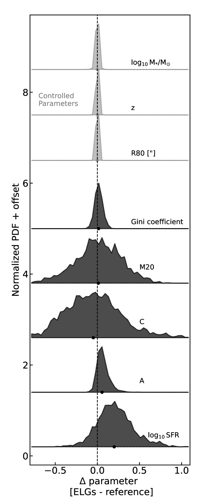
We calculate the differences between the physical and morphological parameters of DESI ELGs and that of overall star-forming galaxies from the COSMOS-ZEST sample at the similar redshifts, stellar mass, and sizes. This analysis allows us to remove the correlations driven by these three parameters. More specifically, for each DESI ELG, we use at least 10 COSMOS-ZEST galaxies as references with redshift difference , stellar mass difference , and size difference . If less than 10 COSMOS-ZEST galaxies are found, we increase the conditions until there are at least 10 galaxies within the selection. Finally, for each ELG, we calculate the difference between the ELG parameter values, SFR, A, G, M20, and C, and the median values of their references as , , , , respectively.
Figure 7 shows the normalized probability density distributions of the excess values of the parameters. The top three parameters are the controlled parameters, stellar mass, redshift, and size (R80). By construction, the distributions are narrow and center around 0. The lower 5 parameters are the morphological parameters, G, M20, C, A, and the SFR values. We find that while there are mild positive excess of G and M20 parameters and on average lower C parameter in comparison to the reference galaxies, the most significant difference is the asymmetric parameter A. The majority () of ELGs have the asymmetric parameter A values higher than the reference galaxies with , a trend similar to the trend of the SFR with ELGs with .
To first explore the correlations between parameters, Table 1 shows the Spearman’s correlation coefficients () between and the spectral PCA coefficient 1 and 2 and the excess values of morphological parameters with the uncertainties estimated by bootstrapping the sample 1000 times. We order the parameters according to their values of Spearman’s correlation coefficients. The results show that
-
•
the correlates with with the highest absolute value among the parameters;
-
•
the second parameter with high value is the line profile coefficient, . We note that between and is . This demonstrates that the correlation between and is not driven by stellar mass.
-
•
, , and parameters also have some correlations with .
These results demonstrate that of DESI ELGs correlates with both the morphological structures and the spectral profiles of galaxies.
To better understand the interplay between the shape of galaxies and the line profiles, Table 2 shows the between and and the excess values of morphological parameters with the uncertainties estimated by bootstrapping the sample 1000 times. As can be seen, and correlate the most with the ( detection) and with other morphological parameters are consistent with no detection (). In other words, based on the values of different parameter pairs, we find that there is a relationship between , , , and .
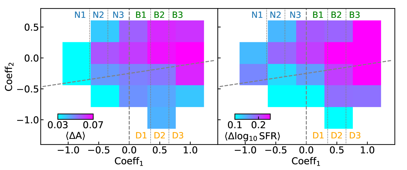
We estimate the median and as a function of and to quantify the relationship. The results are shown in the upper panels of Figure 8, indicating that both median (left panel) and median (right panel) increase from negative to positive and from negative to positive .
We also separate the parameter space into 9 regions based on general classification shown in Figure 2:
-
•
Narrow region: N1 (), N2 (), and N3 ();
-
•
Broad region: B1 (), B2 (), B3 ();
-
•
Double-peak region: D1 (), D2 (), D3 ().
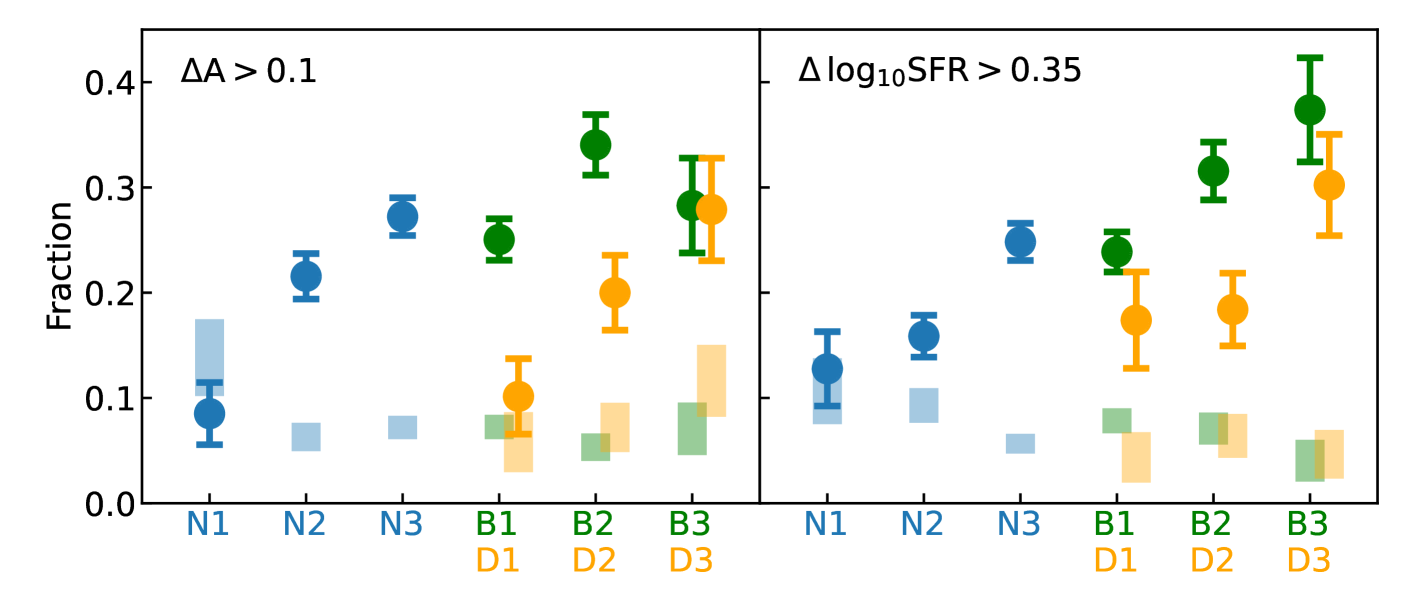
We calculate the fraction of ELGs with high and in each region. The lower panels of Figure 8 summarize the results. The lower left panel show the fractions for . We find that the fractions of ELGs with high increase from the narrow region () to the broad region (). The fractions can increase by a factor of 3 from to . Moreover, for ELGs with , the fraction is higher for ELGs in the broad region () than in the double-peak region (). The lower right panel shows the same measurements with . The overall trends of are consistent with , showing that ELGs with line profiles in the broad region (B) have relatively higher asymmetry morphology and higher SFR than their reference star-forming galaxies with similar stellar mass, sizes and at the same redshifts. In addition, we perform the same analysis for a control sample which consists of star-forming galaxies from the COSMOS-ZEST sample selected to have similar stellar mass, redshifts, and sizes as the properties of DESI ELGs with , and respectively. The color boxes in the lower panels of Figure 8 show the results, indicating that the DESI ELGs have preferentially higher and than typical star-forming galaxies.
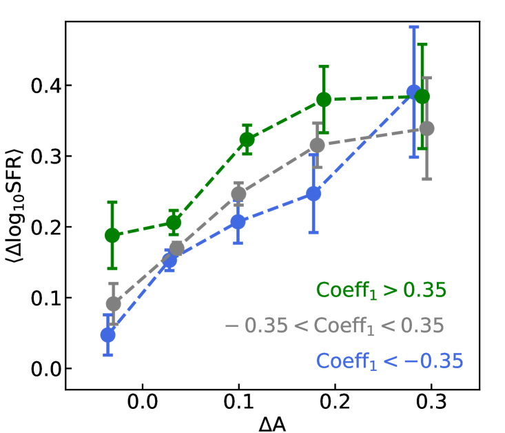
Finally, we quantify the median as a function of and line profiles with the results shown in Figure 9. The blue and green data points are measurements from ELGs with and respectively. The grey data points show the measurements in between. Here we only include ELGs within the narrow and broad regions with . The measurements indicate that there is a general correlation between and which has the same slope but different offsets for galaxies with different . With similar values, DESI ELGs with broader [OII] lines have, on average, 0.1 dex higher than those with narrow [OII] lines. This again illustrates the connection between [OII] line profiles, and of DESI ELGs.
5 Discussion
5.1 The physical mechanisms driving the relationship between SFR, asymmetry, and line profiles
Utilizing data from the DESI spectroscopic observations and the COSMOS multi-wavelength deep images, we find a relationship between three parameters of DESI ELGs, excess SFR (), the asymmetry of galaxy shape (), and the [OII] line profiles. In the following, we discuss two scenarios that can possibly explain the observed relationship.
Merger scenario: The merging of galaxies has been considered as one of the crucial processes that can transform star-forming galaxies into passive ones. Theoretical works have shown that when two gas-rich galaxies merge, gas flows into the centers of the galaxies and trigger excess star-formation activities (e.g., Hopkins et al., 2008; Lotz et al., 2008; Patton et al., 2020; Bottrell et al., 2023). This merger-induced star-formation activities have also been supported by observational studies. Various observational approaches have been used to identify merging galaxies. For example, making use of data from the Sloan Digital Sky Surveys, one can identify galaxy pairs with a range of impact parameters and use such a sample to explore the difference of the SFR compared with the SFR of controlled isolated galaxies with similar mass (e.g. Ellison et al., 2008, 2010; Behroozi et al., 2015). Another approach is to use the morphological parameters of galaxies derived from imaging datasets to identify possible shape features induced by merging events, such as tidal structures and/or asymmetry (e.g., Lotz et al., 2008; Yesuf et al., 2021). Both simulations and observations have shown that merging events at the closest separation enhance the SFR by approximately a factor of 2 with a fixed stellar mass.
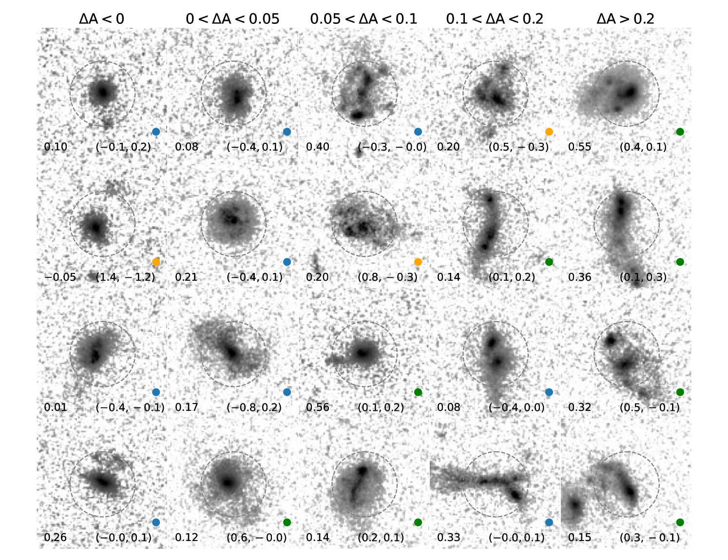
Our results can be explained by this galaxy merger scenario. The excess asymmetry value indicates that a sizable fraction of DESI ELGs are disturbed galaxies, e.g. there are approximately of DESI ELGs with , while there are only of the controlled sample with (lower panels of Figure 8). Figure 10 shows the HST ACS F814W images of randomly selected DESI ELGs as a function of . For most of the galaxies with , two or multi clumpy structures can be observed at small scales () with disturbed and possibly tidal features. The correlation between and values provide a further support on this merger scenario — when two interacting galaxies are at a close distance, the emission lines of the two galaxies are included in a single DESI fiber (12 kpc in diameter at ) with a moderate line-of-sight velocity difference which will produce a [O II] line profile broader than a typical isolated star-forming galaxy with similar stellar mass. The three observational properties of DESI ELGs, the line profile, the asymmetry of galaxy shape, and the excess SFR, can be all fit within the merger scenario simultaneously.
Disk instability scenario: Another possibility is that the multi clumpy structures shown in Figure 10 are star-forming regions formed due to disk instability (e.g., Dekel et al., 2009; Mandelker et al., 2014) in a single galaxy. Previous studies (e.g., Guo et al., 2015; Murata et al., 2014; Martin et al., 2023; Sattari et al., 2023) have shown that the clumpy fraction, the ratio between the number of star-forming galaxies with at least one off-center clump and the total number of star-forming galaxies, roughly peaks between and , overlapping the redshift region of the DESI ELGs, and correlates with SFR with a fixed stellar mass. Bright star-forming clumpy structures can lead to asymmetric light distribution with possible associated emission lines (e.g., Fisher et al., 2017; Oliva-Altamirano et al., 2018) that contribute to the emission line profiles. Moreover, the disk instability is expected to drive turbulent which in turn enhances gas velocity dispersion in galaxies (e.g., Goldbaum et al., 2016). Therefore, this scenario can also produce correlations between , , and line profiles as observed for DESI ELGs.
The origins of clumpy structures observed in high-redshift galaxies are still under active investigations. Some studies have shown that the clump size and gas kinematics relationship of some clumpy galaxies is consistent with the prediction of the disk instability scenario (e.g., Fisher et al., 2017). However, Ribeiro et al. (2017) have shown that galaxies with only two major clumps tend to have clump mass being inconsistent with the expected mass based on disk instability. The authors argue that galaxies with two major clumps can be ongoing galaxy mergers. In addition, Elmegreen et al. (2021) have shown that the observed appearance of major mergers at high redshifts is similar to the observed appearance of clumpy isolated disk galaxies. These studies indicate the complexity of distinguishing clumps formed by disk instability and galaxy mergers. In the DESI ELG sample, while there are galaxies having only two major clumps, some galaxies have more than two clumps as can be seen in Figure 10. Therefore, it is possible that DESI ELGs include both types of systems.
While estimating the contributions of these two scenarios in the overall DESI ELG population is beyond of the scope of this work, one can combine multi-wavelength deep images with radio observations for spatially resolved gas properties to identify tidal features, characterize the properties of the clumpy structures and resolve the nature of these galaxies.
5.2 The origins of double-peak galaxies
Our results show that while ELGs in the double-peak region tend to have higher velocity offsets between two velocity components than ELGs in the broad region, ELGs in the double-peak region, especially in D1 and D2 regions, have on average lower and than ELGs located in the broad (B) region with and , as shown in Figure 8.
We propose that this difference might be due to the fact that instead of tracing two galaxies during the merging process or galaxies with violent disk instability, there is higher fraction of ELGs in the double-peak region with the velocity components reflecting the rotating disks of the galaxies without undergoing SFR enhancement events. One possible way to explore these two scenarios is to investigate the galaxy inclination and relation of ELGs. The expectation for the rotating disk scenario is that those galaxies tend to be more edge-on with low . On the other hand, the morphology of two merging galaxies with close separation or galaxies with two major clumps can resemble the morphology of edge-on galaxies. Therefore, merging/clumpy galaxies also tend to look like edge-on galaxies but with higher than the rotating disks.
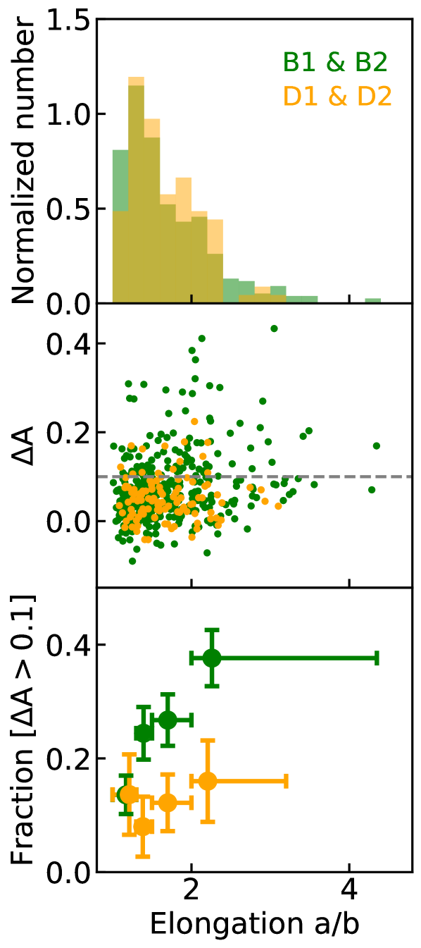
In Figure 11, we examine the distribution of and galaxy inclination, using the elongation parameter, the ratio between the lengths of semi-major and semi-minor axes of galaxies, from HST images as a proxy (Leauthaud et al., 2007). We only select ELGs with to reduce possible effects associated with galaxy mass. The top panel shows the normalized number distributions of the elongation parameter of DESI ELGs in regions and regions indicated by green and orange respectively. The middle panel shows the distribution of as a function of the elongation parameter and the bottom panel shows the fraction of ELGs with as a function of the elongation parameter for the two types of ELGs. We find that ELGs in regions and regions both have a broad range of elongation parameter. The middle and bottom panels show that for ELGs in regions, the fraction of sources with is consistently being across all elongation parameter values. In contrast, the fraction of ELGs in regions with increases with the elongation parameter from 0.2 to 0.4. These observed trends are consistent with the above proposed scenario that mergers/clumpy galaxies tend to have high elongation and high , while rotating disks tend to have high elongation but with low . However, we note that the above results are suggestive and spatially resolved kinematics information is needed to conclusively identify the origins of double-peak emission lines observed in DESI ELGs.
Previous studies have also suggested that double-peak emission lines observed in galaxies are associated with rotating disks at the local Universe. For example, Maschmann et al. (2020) found double-peak emission line galaxies from the SDSS spectroscopic dataset. Based on simulations, Maschmann et al. (2023) concluded that the double-peak emission lines can be originated from the central rotating bars of galaxies or minor mergers. Chen et al. (2016) also found that rotating galaxy discs can explain the double-peak emission lines observed in SDSS disc star-forming galaxies.
5.3 DESI ELG selection for galaxy properties
We now explore the key selection criteria for DESI ELGs which preferentially include galaxies with high SFR and asymmetric morphology. The DESI ELG selections for the main survey are summarized in Table 2 of Raichoor et al. (2023), which includes
-
•
,
-
•
, and
-
•
and color boundaries.
To investigate how these selection conditions affect the galaxy properties, we use the COSMOS-ZEST galaxy sample and cross-match the sample with the photometric catalog444DR10 https://www.legacysurvey.org/dr10/catalogs/ from the DESI Legacy Imaging Surveys (Dey et al., 2019) to obtain the photometric information used in the DESI target selections. We then select star-forming galaxies with , (the parameter space that covers the main DESI ELGs) and . For each star-forming galaxy, we follow the same procedure for estimating and as the DESI ELG sample by searching for at least 10 galaxies as references with redshift difference , stellar mass difference , and size difference and increasing the conditions if less than 10 galaxies are found. The and are the differences between the values of the galaxies and the median values of the reference galaxies.
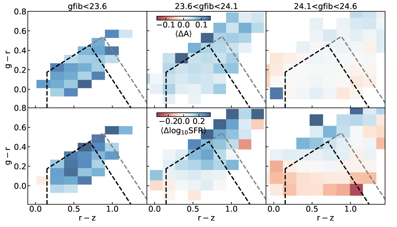
With and information, we calculate the median and as a function of , colors, and . The upper panels of Figure 12 show the median values across the and color space with (left panel), (middle panel) and (right panel). The black dashed lines are the boundaries for the DESI ELGs LOP sample and the grey dashed lines are the extended region for the VLO sample. As can be seen, galaxies that are brighter in preferentially have higher values. A similar trend is observed for as shown in the lower panels of Figure 12 indicating the median values of galaxies. We note that while there is no strong correlation between and galaxy colors, a correlation between and galaxy colors can be observed in the middle and right panels. Therefore, we conclude that the g-band fiber magnitude selection is the primary factor for selecting galaxies with more disturbed morphology and higher SFR than the overall star-forming galaxy population at the same redshifts and the (g-r, r-z) color selections are an additional factor modulating the SFR. Note that while reaches the limiting magnitude of the Legacy Surveys (Dey et al., 2019) with larger uncertainties, we have performed the same analysis with g, r, z-band images with depths magnitude from Hyper Suprime-Cam (Aihara et al., 2018, 2019) in the COSMOS2020 catalog which yield consistent results.
5.4 Implications for DESI ELG clustering measurements
Recent studies have shown that in order to reproduce the DESI ELG clustering properties, especially the small-scale signals (), and obtain physically motivated ELG-halo connection models, additional parameters are required in the halo occupation distribution (HOD) modeling (e.g., Gao et al., 2023; Yuan et al., 2023; Rocher et al., 2023; Gao et al., 2024). These results indicate that the abundance of satellite ELGs in the halos depends on the properties of the central ELGs — a phenomenon called ”conformity” (Wechsler & Tinker, 2018, for a review).
By exploring the properties of ELGs at and their morphology with COSMOS dataset, Yuan et al. (2023) postulate that such conformity signals are driven by galaxy merging induced star formation in both central and satellite galaxies. Our findings of the relationship between SFR, galaxy morphology and the line profiles are consistent with this scenario. In addition, the small-scale enhancement of the clustering amplitude of DESI ELGs is aligned with the results of simulations focusing on galaxy mergers (e.g., Wetzel et al., 2009).
In addition to the behavior of spatial clustering properties of DESI ELGs, Rocher et al. (2023) find that DESI ELGs have an unexpected clustering property in velocity space. They find that on average, the velocity dispersion of the satellite DESI ELGs is larger than the velocity dispersion of dark matter particles by . We argue that this observed property is likely associated with spectral profiles of DESI ELGs having two velocity components along the sightlines. As shown in Figure 4, for two redshift systems, the median value of the line of sight velocity offsets is . However, the current pipeline typically determines the redshift in the middle of the two velocity components. In this case, this can possibly introduce a velocity offset of the central galaxy redshifts systematically and adds additional velocity dispersion in the relative velocities between centrals and satellites.
Here we consider a simple case to quantify possible signals. Assuming that the dark matter halo mass of ELGs is (e.g., Rocher et al., 2023) with the corresponding velocity dispersion of dark matter particles being , adding a systematic offset in the velocity measurements will increase the estimated velocity dispersion by , which is similar to the results in Rocher et al. (2023). This demonstrates that this redshift determination effect can be responsible for at least part of the apparent excess velocity dispersion of the satellite galaxies and it needs to be taken into account for the clustering measurements in velocity space.
6 Conclusions
By performing PCA on spectra of ELGs at from DESI Early Data Release, we decomposed [OII] profiles based on the derived PCA eigen-spectra and explored the diversity of [OII] line profiles in low-dimensional coefficient space. We further utilized the physical and morphological properties of galaxies in the COSMOS field and investigated the relationship between [OII] line profiles and the properties of the galaxies. Our main findings are summarized as follows:
-
•
We find that the first two eigen-spectra, which correspond to the line width (1st) and the peakedness (2nd) of [OII] doublet lines, can explain of the total variance of [OII] line profiles. Using the coefficients of these two eigen-spectra, we show that DESI ELGs can be classified into at least three types with narrow [OII] lines, broad [OII] lines, and two-redshift systems, demonstrating the diversity of [OII] line profiles.
-
•
Combining PCA results with the galaxy physical properties from the COSMOS2020 catalog, we find that ELGs with broader line profiles tend to have higher stellar mass and SFR. Moreover, by fixing stellar mass, we find that ELGs with broader line profiles have higher median SFR. We also find that DESI ELGs preferentially have higher SFR than the average SFR of the star-forming galaxies at the similar redshifts. These trends are observed across the entire redshift range of DESI ELGs from to .
-
•
We include the morphological properties of DESI ELGs derived from HST ACS images and quantify the enhancement of various properties, including SFR and shape properties, of DESI ELGs with respect to the reference star-forming galaxies with similar stellar mass, sizes, and redshifts. We find that correlates the most with and with Spearman’s correlation coefficients with 0.31 and 0.16 respectively. Moreover, has the highest correlation coefficient with ( with detection) than with other morphological parameters.
-
•
The median and and the fraction of high and high as a function of and both show that ELGs with broad line profiles have higher and than ELGs with narrow or double-peak line profiles. This result reveals an underlying relationship between , , and line profiles.
-
•
We show that ELGs with high have on average dex enhancement of the SFR than ELGs with low and the can further contribute to the enhancement of SFR by dex.
Finally, we argue that this inter-relationship between the line profiles, physical and morphological properties of DESI ELGs can be naturally explained by both the galaxy merger and disk instability star-forming clumps scenarios.
The results of this work show that the large DESI spectroscopic dataset opens a new window for statistically investigating the galaxy physical properties and how the mechanism drives galaxy evolution at . The combination of the DESI data and upcoming imaging datasets provided by space telescopes, such as Euclid (Euclid Collaboration et al., 2022) and the Roman Space Telescope (Akeson et al., 2019), will further offer a large galaxy sample with both kinematics and morphological information of galaxies for galaxy evolution science.
Understanding how the physical properties of galaxies link to the properties of dark matter halos and the large-scale environments is crucial for obtaining precise cosmological measurements. Recent galaxy clustering results of DESI ELGs indicate that the standard galaxy-halo connection models are insufficient to describe small-scale clustering measurements in both spatial and velocity space. As demonstrated in this work, this is possibly due to the nature of DESI ELGs and the redshift determination effect due to their diverse line profiles. It will be informative to perform clustering measurements as a function of emission line profiles and obtain a better understanding of small-scale clustering properties of the DESI ELG population. This approach can be used to utilize the hidden spectral information from the ongoing and upcoming cosmological spectroscopic surveys, including PFS (Takada et al., 2014), Euclid (Euclid Collaboration et al., 2022), the Roman Space Telescope (Akeson et al., 2019), and the next-generation surveys, e.g., DESI-II and Spec-5 experiments (Schlegel et al., 2022), that use emission line galaxies as primary tracers for the large-scale structure of the Universe.
Data Availability
All data points shown in the figures are available at Zenodo.
Appendix A Removing active galactic nuclei
It is possible that a fraction of DESI ELGs having actively accreting supermassive black holes (active galactic nuclei, AGN) which can produce [OII] lines. To eliminate the complexity due to the AGN contributions, we utilize available line information obtained via the FastSpecFit555https://fastspecfit.readthedocs.io/en/latest/index.html algorithm developed by Moustakas et al. (2024). We identify DESI ELGs that satisfy any of the following conditions and remove them from our analysis:
| (A1) |
| (A2) |
| (A3) |
The first condition A1 follows the condition used in Zakamska et al. (2003) and Reyes et al. (2008) for selecting Type II quasars at where only and lines are accessible in the optical wavelength coverage. In Zakamska et al. (2003), the selections are and . In our condition, we reduce the line ratio by 0.1 dex and the line width by 100 km/s so that our selection is conservative.
The second condition, the signal-to-noise cut of MgII emission line (A2), is used to remove ELG spectra with possible broad MgII emission lines originated from quasars, e.g., the missing quasar population in Alexander et al. (2023).
Appendix B Morphology parameters as a function of line profiles
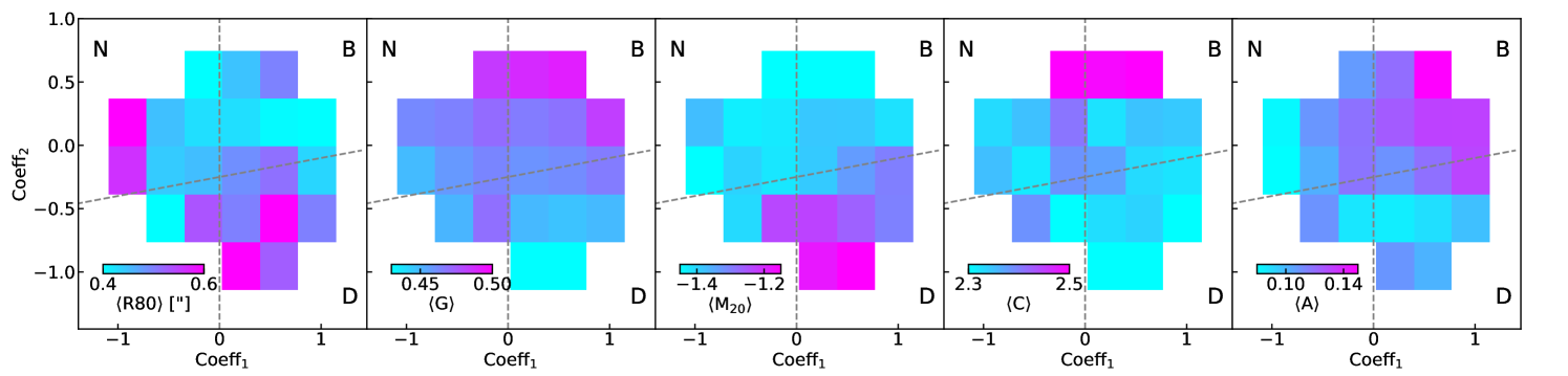
Here we summarize the relationships between the morphological parameters and the line profiles. Figure 13 shows the median values of the morphological parameters, galaxy size (R80), Gini coefficient (G), the second-order moment of the brightest pixels (M20), concentration (C), and asymmetry (A) from left to right respectively, as a function of and . These results are based on the DESI-ZEST sample.
Trends can be observed from Figure 13. First, DESI ELGs in the double-peak region tend to have larger sizes than DESI ELGs in other regions as shown in the first panel. This is consistent with the fact that DESI ELGs in the double-peak region also have higher stellar mass. Correlating with R80, the M20 values also tend to be larger in the double-peak region. We note that the DESI ELGs with have on average lower redshifts and therefore have larger observed sizes. Second, Gini coefficient (G) and asymmetry parameter (A) behave similarly with higher median values in the broad region, indicating that DESI ELGs in the broad region tend to have relatively disturbed morphology. Finally, the concentration C anti-correlates with M20, having the highest median values for DESI ELGs with high . These internal correlations between parameters are consistent with the results summarized in Scarlata et al. (2007). We note that while these morphological parameters all have some dependencies with the line profiles, we focus on the asymmetry parameter in this work given that the excess asymmetry parameter yields the highest Spearman’s correlation coefficients with and and as shown in Section 4.
References
- Abraham et al. (2003) Abraham, R. G., van den Bergh, S., & Nair, P. 2003, ApJ, 588, 218. doi:10.1086/373919
- Aihara et al. (2018) Aihara, H., Arimoto, N., Armstrong, R., et al. 2018, PASJ, 70, S4. doi:10.1093/pasj/psx066
- Aihara et al. (2019) Aihara, H., AlSayyad, Y., Ando, M., et al. 2019, PASJ, 71, 114. doi:10.1093/pasj/psz103
- Alexander et al. (2023) Alexander, D. M., Davis, T. M., Chaussidon, E., et al. 2023, AJ, 165, 124. doi:10.3847/1538-3881/acacfc
- Anand et al. (2024) Anand, A., Guy, J., Bailey, S., et al. 2024, arXiv:2405.19288. doi:10.48550/arXiv.2405.19288
- Akeson et al. (2019) Akeson, R., Armus, L., Bachelet, E., et al. 2019, arXiv:1902.05569. doi:10.48550/arXiv.1902.05569
- Astropy Collaboration et al. (2013) Astropy Collaboration, Robitaille, T. P., Tollerud, E. J., et al. 2013, A&A, 558, A33. doi:10.1051/0004-6361/201322068
- Astropy Collaboration et al. (2018) Astropy Collaboration, Price-Whelan, A. M., Sipőcz, B. M., et al. 2018, AJ, 156, 123. doi:10.3847/1538-3881/aabc4f
- Astropy Collaboration et al. (2022) Astropy Collaboration, Price-Whelan, A. M., Lim, P. L., et al. 2022, ApJ, 935, 167. doi:10.3847/1538-4357/ac7c74
- Bailey (2012) Bailey, S. 2012, PASP, 124, 1015. doi:10.1086/668105
- Bailey et al. (2023) Bailey, S. et al. in prep
- Behroozi et al. (2015) Behroozi, P. S., Zhu, G., Ferguson, H. C., et al. 2015, MNRAS, 450, 1546. doi:10.1093/mnras/stv728
- Bertin & Arnouts (1996) Bertin, E. & Arnouts, S. 1996, A&AS, 117, 393. doi:10.1051/aas:1996164
- Blake et al. (2011) Blake, C., Kazin, E. A., Beutler, F., et al. 2011, MNRAS, 418, 1707. doi:10.1111/j.1365-2966.2011.19592.x
- Bottrell et al. (2023) Bottrell, C., Yesuf, H. M., Popping, G., et al. 2023, MNRAS. doi:10.1093/mnras/stad2971
- Brammer et al. (2008) Brammer, G. B., van Dokkum, P. G., & Coppi, P. 2008, ApJ, 686, 1503. doi:10.1086/591786
- Brodzeller et al. (2023) Brodzeller, A., Dawson, K., Bailey, S., et al. 2023, AJ, 166, 66. doi:10.3847/1538-3881/ace35d
- Chabrier (2003) Chabrier, G. 2003, PASP, 115, 763. doi:10.1086/376392
- Chaussidon et al. (2023) Chaussidon, E., Yèche, C., Palanque-Delabrouille, N., et al. 2023, ApJ, 944, 107. doi:10.3847/1538-4357/acb3c2
- Chen et al. (2016) Chen, Y.-M., Gu, Q.-S., Tremonti, C. A., et al. 2016, MNRAS, 459, 3861. doi:10.1093/mnras/stw942
- Cleri et al. (2023) Cleri, N. J., Yang, G., Papovich, C., et al. 2023, ApJ, 948, 112. doi:10.3847/1538-4357/acc1e6
- Comparat et al. (2013) Comparat, J., Kneib, J.-P., Bacon, R., et al. 2013, A&A, 559, A18. doi:10.1051/0004-6361/201322452
- Comparat et al. (2015) Comparat, J., Richard, J., Kneib, J.-P., et al. 2015, A&A, 575, A40. doi:10.1051/0004-6361/201424767
- Conselice (2014) Conselice, C. J. 2014, ARA&A, 52, 291. doi:10.1146/annurev-astro-081913-040037
- Cooper et al. (2023) Cooper, A. P., Koposov, S. E., Allende Prieto, C., et al. 2023, ApJ, 947, 37. doi:10.3847/1538-4357/acb3c0
- COSMOS team (2007) COSMOS team 2007, COSMOS Zurich Structure & Morphology Catalog, v1, IPAC, doi:10.26131/IRSA160
- Dawson et al. (2016) Dawson, K. S., Kneib, J.-P., Percival, W. J., et al. 2016, AJ, 151, 44. doi:10.3847/0004-6256/151/2/44
- Delchambre (2015) Delchambre, L. 2015, MNRAS, 446, 3545. doi:10.1093/mnras/stu2219
- Dekel et al. (2009) Dekel, A., Sari, R., & Ceverino, D. 2009, ApJ, 703, 785. doi:10.1088/0004-637X/703/1/785
- DESI Collaboration et al. (2016a) DESI Collaboration, Aghamousa, A., Aguilar, J., et al. 2016, arXiv:1611.00036. doi:10.48550/arXiv.1611.00036
- DESI Collaboration et al. (2016b) DESI Collaboration, Aghamousa, A., Aguilar, J., et al. 2016, arXiv:1611.00037. doi:10.48550/arXiv.1611.00037
- DESI Collaboration et al. (2022) DESI Collaboration, Abareshi, B., Aguilar, J., et al. 2022, AJ, 164, 207. doi:10.3847/1538-3881/ac882b
- DESI Collaboration et al. (2024a) DESI Collaboration, Adame, A. G., Aguilar, J., et al. 2024, AJ, 167, 62. doi:10.3847/1538-3881/ad0b08
- DESI Collaboration et al. (2024b) DESI Collaboration, Adame, A. G., Aguilar, J., et al. 2024, AJ, 168, 58. doi:10.3847/1538-3881/ad3217
- Dey et al. (2019) Dey, A., Schlegel, D. J., Lang, D., et al. 2019, AJ, 157, 168. doi:10.3847/1538-3881/ab089d
- Drinkwater et al. (2010) Drinkwater, M. J., Jurek, R. J., Blake, C., et al. 2010, MNRAS, 401, 1429. doi:10.1111/j.1365-2966.2009.15754.x
- Eisenstein et al. (2005) Eisenstein, D. J., Zehavi, I., Hogg, D. W., et al. 2005, ApJ, 633, 560. doi:10.1086/466512
- Euclid Collaboration et al. (2022) Euclid Collaboration, Scaramella, R., Amiaux, J., et al. 2022, A&A, 662, A112. doi:10.1051/0004-6361/202141938
- Ellison et al. (2008) Ellison, S. L., Patton, D. R., Simard, L., et al. 2008, AJ, 135, 1877. doi:10.1088/0004-6256/135/5/1877
- Ellison et al. (2010) Ellison, S. L., Patton, D. R., Simard, L., et al. 2010, MNRAS, 407, 1514. doi:10.1111/j.1365-2966.2010.17076.x
- Elmegreen et al. (2021) Elmegreen, D. M., Elmegreen, B. G., Whitmore, B. C., et al. 2021, ApJ, 908, 121. doi:10.3847/1538-4357/abd541
- Fisher et al. (2017) Fisher, D. B., Glazebrook, K., Abraham, R. G., et al. 2017, ApJ, 839, L5. doi:10.3847/2041-8213/aa6478
- Gao et al. (2023) Gao, H., Jing, Y. P., Gui, S., et al. 2023, ApJ, 954, 207. doi:10.3847/1538-4357/ace90a
- Gao et al. (2024) Gao, H., Jing, Y. P., Xu, K., et al. 2024, ApJ, 961, 74. doi:10.3847/1538-4357/ad09d6
- Goldbaum et al. (2016) Goldbaum, N. J., Krumholz, M. R., & Forbes, J. C. 2016, ApJ, 827, 28. doi:10.3847/0004-637X/827/1/28
- Gould et al. (2023) Gould, K. M. L., Brammer, G., Valentino, F., et al. 2023, AJ, 165, 248. doi:10.3847/1538-3881/accadc
- Guo et al. (2015) Guo, Y., Ferguson, H. C., Bell, E. F., et al. 2015, ApJ, 800, 39. doi:10.1088/0004-637X/800/1/39
- Guy et al. (2023) Guy, J., Bailey, S., Kremin, A., et al. 2023, AJ, 165, 144. doi:10.3847/1538-3881/acb212
- Hahn et al. (2023) Hahn, C., Wilson, M. J., Ruiz-Macias, O., et al. 2023, AJ, 165, 253. doi:10.3847/1538-3881/accff8
- Harris et al. (2020) Harris, C.R., Millman, K.J., van der Walt, S.J. et al. 2020, Nature 585, 357–362. doi: 10.1038/s41586-020-2649-2
- Hinshaw et al. (2013) Hinshaw, G., Larson, D., Komatsu, E., et al. 2013, ApJS, 208, 19. doi:10.1088/0067-0049/208/2/19
- Hopkins et al. (2008) Hopkins, P. F., Hernquist, L., Cox, T. J., et al. 2008, ApJS, 175, 356. doi:10.1086/524362
- Hunter (2007) Hunter, J. D. 2007, Computing in Science & Engineering, 9, 90. doi:10.1109/MCSE.2007.55
- Ilbert et al. (2006) Ilbert, O., Arnouts, S., McCracken, H. J., et al. 2006, A&A, 457, 841. doi:10.1051/0004-6361:20065138
- Jolliffe (2002) Jolliffe, Ian, 2002, Principal component analysis, 338-372, Publisher Springer New York
- Kassin et al. (2012) Kassin, S. A., Weiner, B. J., Faber, S. M., et al. 2012, ApJ, 758, 106. doi:10.1088/0004-637X/758/2/106
- Kaasinen et al. (2017) Kaasinen, M., Bian, F., Groves, B., et al. 2017, MNRAS, 465, 3220. doi:10.1093/mnras/stw2827
- Kennicutt (1998) Kennicutt, R. C. 1998, ARA&A, 36, 189. doi:10.1146/annurev.astro.36.1.189
- Kennicutt et al. (2009) Kennicutt, R. C., Hao, C.-N., Calzetti, D., et al. 2009, ApJ, 703, 1672. doi:10.1088/0004-637X/703/2/1672
- Kewley et al. (2019) Kewley, L. J., Nicholls, D. C., & Sutherland, R. S. 2019, ARA&A, 57, 511. doi:10.1146/annurev-astro-081817-051832
- Koekemoer et al. (2007) Koekemoer, A. M., Aussel, H., Calzetti, D., et al. 2007, ApJS, 172, 196. doi:10.1086/520086
- Kriek & Conroy (2013) Kriek, M. & Conroy, C. 2013, ApJ, 775, L16. doi:10.1088/2041-8205/775/1/L16
- Lan et al. (2023) Lan, T.-W., Tojeiro, R., Armengaud, E., et al. 2023, ApJ, 943, 68. doi:10.3847/1538-4357/aca5fa
- Lang et al. (2016) Lang, D., Hogg, D. W., & Mykytyn, D. 2016, Astrophysics Source Code Library. ascl:1604.008
- Law et al. (2022) Law, D. R., Belfiore, F., Bershady, M. A., et al. 2022, ApJ, 928, 58. doi:10.3847/1538-4357/ac5620
- Leauthaud et al. (2007) Leauthaud, A., Massey, R., Kneib, J.-P., et al. 2007, ApJS, 172, 219. doi:10.1086/516598
- Levi et al. (2013) Levi, M., Bebek, C., Beers, T., et al. 2013, arXiv:1308.0847
- Lotz et al. (2004) Lotz, J. M., Primack, J., & Madau, P. 2004, AJ, 128, 163. doi:10.1086/421849
- Lotz et al. (2008) Lotz, J. M., Jonsson, P., Cox, T. J., et al. 2008, MNRAS, 391, 1137. doi:10.1111/j.1365-2966.2008.14004.x
- Madau & Dickinson (2014) Madau, P. & Dickinson, M. 2014, ARA&A, 52, 415. doi:10.1146/annurev-astro-081811-125615
- Maddox (2018) Maddox, N. 2018, MNRAS, 480, 5203. doi:10.1093/mnras/sty2201
- Mai et al. (2024) Mai, Y., Croom, S. M., Wisnioski, E., et al. 2024, MNRAS. doi:10.1093/mnras/stae2033
- Mandelker et al. (2014) Mandelker, N., Dekel, A., Ceverino, D., et al. 2014, MNRAS, 443, 3675. doi:10.1093/mnras/stu1340
- Martin et al. (2023) Martin, A., Guo, Y., Wang, X., et al. 2023, ApJ, 955, 106. doi:10.3847/1538-4357/aced3e
- Maschmann et al. (2020) Maschmann, D., Melchior, A.-L., Mamon, G. A., et al. 2020, A&A, 641, A171. doi:10.1051/0004-6361/202037868
- Maschmann et al. (2023) Maschmann, D., Halle, A., Melchior, A.-L., et al. 2023, A&A, 670, A46. doi:10.1051/0004-6361/202244746
- McCracken et al. (2012) McCracken, H. J., Milvang-Jensen, B., Dunlop, J., et al. 2012, A&A, 544, A156. doi:10.1051/0004-6361/201219507
- Miller et al. (2023) Miller, T. N., Doel, P., Gutierrez, G., et al. 2023, arXiv:2306.06310. doi:10.48550/arXiv.2306.06310
- Moustakas et al. (2006) Moustakas, J., Kennicutt, R. C., & Tremonti, C. A. 2006, ApJ, 642, 775. doi:10.1086/500964
- Moustakas et al. (2013) Moustakas, J., Coil, A. L., Aird, J., et al. 2013, ApJ, 767, 50. doi:10.1088/0004-637X/767/1/50
- Moustakas et al. (2023) Moustakas, J., Lang, D., Dey, A., et al. 2023, ApJS, 269, 3. doi:10.3847/1538-4365/acfaa2
- Moustakas et al. (2024) Moustakas, J. et al. in prep.
- Murata et al. (2014) Murata, K. L., Kajisawa, M., Taniguchi, Y., et al. 2014, ApJ, 786, 15. doi:10.1088/0004-637X/786/1/15
- Myers et al. (2023) Myers, A. D., Moustakas, J., Bailey, S., et al. 2023, AJ, 165, 50. doi:10.3847/1538-3881/aca5f9
- Oliva-Altamirano et al. (2018) Oliva-Altamirano, P., Fisher, D. B., Glazebrook, K., et al. 2018, MNRAS, 474, 522. doi:10.1093/mnras/stx2797
- Osterbrock & Ferland (2006) Osterbrock, D. E. & Ferland, G. J. 2006, Astrophysics of gaseous nebulae and active galactic nuclei, 2nd. ed. by D.E. Osterbrock and G.J. Ferland. Sausalito, CA: University Science Books, 2006
- Patton et al. (2020) Patton, D. R., Wilson, K. D., Metrow, C. J., et al. 2020, MNRAS, 494, 4969. doi:10.1093/mnras/staa913
- Raichoor et al. (2021) Raichoor, A., de Mattia, A., Ross, A. J., et al. 2021, MNRAS, 500, 3254. doi:10.1093/mnras/staa3336
- Raichoor et al. (2023) Raichoor, A., Moustakas, J., Newman, J. A., et al. 2023, AJ, 165, 126. doi:10.3847/1538-3881/acb213
- Raichoor et al. (2024) Raichoor, A., et al. in prep.
- Reyes et al. (2008) Reyes, R., Zakamska, N. L., Strauss, M. A., et al. 2008, AJ, 136, 2373. doi:10.1088/0004-6256/136/6/2373
- Ribeiro et al. (2017) Ribeiro, B., Le Fèvre, O., Cassata, P., et al. 2017, A&A, 608, A16. doi:10.1051/0004-6361/201630057
- Rocher et al. (2023) Rocher, A., Ruhlmann-Kleider, V., Burtin, E., et al. 2023, J. Cosmology Astropart. Phys, 2023, 016. doi:10.1088/1475-7516/2023/10/016
- Sattari et al. (2023) Sattari, Z., Mobasher, B., Chartab, N., et al. 2023, ApJ, 951, 147. doi:10.3847/1538-4357/acd5d6
- Scarlata et al. (2007) Scarlata, C., Carollo, C. M., Lilly, S., et al. 2007, ApJS, 172, 406. doi:10.1086/516582
- Schlafly et al. (2023) Schlafly, E. F., Kirkby, D., Schlegel, D. J., et al. 2023, arXiv:2306.06309. doi:10.48550/arXiv.2306.06309
- Schlegel et al. (1998) Schlegel, D. J., Finkbeiner, D. P., & Davis, M. 1998, ApJ, 500, 525. doi:10.1086/305772
- Schlegel et al. (2022) Schlegel, D. J., Ferraro, S., Aldering, G., et al. 2022, arXiv:2209.03585. doi:10.48550/arXiv.2209.03585
- Scoville et al. (2007) Scoville, N., Abraham, R. G., Aussel, H., et al. 2007, ApJS, 172, 38. doi:10.1086/516580
- Scoville et al. (2007) Scoville, N., Aussel, H., Brusa, M., et al. 2007, ApJS, 172, 1. doi:10.1086/516585
- Silber et al. (2023) Silber, J. H., Fagrelius, P., Fanning, K., et al. 2023, AJ, 165, 9. doi:10.3847/1538-3881/ac9ab1
- Suzuki (2006) Suzuki, N. 2006, ApJS, 163, 110. doi:10.1086/499272
- Taghizadeh-Popp et al. (2012) Taghizadeh-Popp, M., Heinis, S., & Szalay, A. S. 2012, ApJ, 755, 143. doi:10.1088/0004-637X/755/2/143
- Takada et al. (2014) Takada, M., Ellis, R. S., Chiba, M., et al. 2014, PASJ, 66, R1. doi:10.1093/pasj/pst019
- Terlouw and Vogelaar (2014) Terlouw, J.P. and Vogelaar, M. G. R. 2014, http://www.astro.rug.nl/software/kapteyn/
- Übler et al. (2019) Übler, H., Genzel, R., Wisnioski, E., et al. 2019, ApJ, 880, 48. doi:10.3847/1538-4357/ab27cc
- Vanderplas et al. (2012) Vanderplas, J.T., Connolly, A.J., Ivezić, Ž. and Gray, A., proc. of CIDU, pp. 47-54, 2012. doi:10.1109/CIDU.2012.6382200
- van der Wel et al. (2014) van der Wel, A., Franx, M., van Dokkum, P. G., et al. 2014, ApJ, 788, 28. doi:10.1088/0004-637X/788/1/28
- Virtanen et al. (2020) Virtanen, P., Gommers, R., Oliphant, T.E., et al. 2020, Nature Methods, 17(3), 261-272. doi: 10.1038/s41592-019-0686-2
- Yesuf et al. (2021) Yesuf, H. M., Ho, L. C., & Faber, S. M. 2021, ApJ, 923, 205. doi:10.3847/1538-4357/ac27a7
- Yip et al. (2004) Yip, C. W., Connolly, A. J., Szalay, A. S., et al. 2004, AJ, 128, 585. doi:10.1086/422429
- Yuan et al. (2023) Yuan, S., Wechsler, R. H., Wang, Y., et al. 2023, arXiv:2310.09329. doi:10.48550/arXiv.2310.09329
- Weaver et al. (2022) Weaver, J. R., Kauffmann, O. B., Ilbert, O., et al. 2022, ApJS, 258, 11. doi:10.3847/1538-4365/ac3078
- Wechsler & Tinker (2018) Wechsler, R. H. & Tinker, J. L. 2018, ARA&A, 56, 435. doi:10.1146/annurev-astro-081817-051756
- Wetzel et al. (2009) Wetzel, A. R., Cohn, J. D., & White, M. 2009, MNRAS, 394, 2182. doi:10.1111/j.1365-2966.2009.14488.x
- Wright et al. (2010) Wright, E. L., Eisenhardt, P. R. M., Mainzer, A. K., et al. 2010, AJ, 140, 1868. doi:10.1088/0004-6256/140/6/1868
- Zakamska et al. (2003) Zakamska, N. L., Strauss, M. A., Krolik, J. H., et al. 2003, AJ, 126, 2125. doi:10.1086/378610
- Zhou et al. (2023) Zhou, R., Dey, B., Newman, J. A., et al. 2023, AJ, 165, 58. doi:10.3847/1538-3881/aca5fb