Design and Experimental Evaluation of a Hierarchical Controller for an Autonomous Ground Vehicle with Large Uncertainties

The main idea of the MPC-based improved path planning is generating an optimal path by simulating a tracking process using MPC along the original path. The new path is smoother than the original path, and is kinematically feasible for the AGV to follow.

Since only the spatial information is considered in the global path planning stage, a trajectory with a constant velocity is first generated based on the global path $\mathbf{r}=\{r_{i}\}_{0}^{N_{r}}$. In our study, the resolution of the environment map is assumed to be high enough, so the distance between adjacent reference waypoints $r_{k-1}$ and $r_{k}$ is small. The time interval $\Delta t_{k}$ can be approximated by

where the reference velocity of the robot at position $r_{k}$ is set to be a constant value ${v_{c}}$. Based on the time interval $\Delta t_{k}$, the corresponding reference time of each waypoint $r_{k}$ can be expressed as

Then, an MPC-based tracking process is executed on the trajectory $\nu=\{r_{i},T_{i}\}_{0}^{N_{r}}$ to generate a new path. The optimal trajectory tracking control problem at time $T_{k}$ is formulated as

where $J(\cdot)$ is the cost within the finite horizon $H$ and $J_{\textrm{f}}(\cdot)$ is the terminal cost. Here $z$ is the pose of the AGV, and $u$ is the control input which consists of the linear and angular velocities. This optimization problem is solved under several constraints. Eq. (6b) represents the initial state constraint. The initial state $z_{0}$ is given by current state $z(T_{k})$. Eq. (6c) represents the kinematic constraint which is used to predict the motion of the AGV. According to the kinematic equation in (1) and the reference trajectory, the kinematic constraint (6c) can be specified by

Note that in (7), the time interval $\Delta t_{k+i}$ should be small enough to reduce the discretization error. According to (4), it means that the trajectory should be adequately dense. Since the MPC predicts the AGV’s future trajectory within a fixed horizon, a denser trajectory will lead to a higher computational complexity. Therefore, in practice, there exists a tradeoff between the model discretization accuracy and the computational complexity. Besides, Eq. (6d) represents the state and control input constraints, where $\mathbb{Z}$ and $\mathbb{U}$ are the feasible sets for $z$ and $u$, respectively.

In the MPC framework, the cost function needs to be carefully defined to achieve satisfactory performance. For the path smoothing task, both tracking accuracy and smoothness of the control should be considered. Therefore, the complete cost function is designed as

where

and $Q_{i}\in{\mathbb{R}^{3\times 3}}$, $R_{i}\in{\mathbb{R}^{2\times 2}}$, and $S_{i}\in{\mathbb{R}^{2\times 2}}$ are positive definite weighting matrices. The cost function consists of three parts. $\widetilde{z}_{i}$ represents the distance between the state $z$ and the corresponding reference waypoint $r$ at time step $i$, so the first part of the cost function penalizes the distance between the smoothed path and original path within the time horizon $H$. $\widetilde{u}_{i}$ represents the difference between the control input $u$ and the reference velocity $u^{\rm{ref}}$ at time step $i$. Since a constant velocity $v_{c}$ is used to generate the trajectory, here $u^{\rm{ref}}=[v_{c},0]^{\rm{T}}$. $\Delta u_{i}$ represents the variation between two successive control inputs. The third part of the cost function penalizes the fluctuation of the control signal and makes the robot motion smoother.

Note that the optimization problem (6) is non-convex due to the inclusion of the non-convex constraint (6c). In this study, we use the interior point method [28] to solve the non-convex optimization problem (6). This method implements an interior point line search filter to find a local optimal solution. Since our objective is to find an optimal path close to the original path, the original path is leveraged to initialize the optimization problem, which makes it very likely to converge to the global optimal solution. The optimal predicted states $\bf{z}^{*}$ and control inputs $\bf{u}^{*}$ are denoted by

The predicted states $\bf{z}^{*}$ can be regarded as a new path which consists of $H$ waypoints. In the optimization problem, the tracking error and control input fluctuation have been penalized, so the new path should be both close to the original path and smooth enough. What is more, since the kinematic model and the velocity limits are considered during the optimization process, the new path is kinematically and physically feasible for the AGV.

If the prediction horizon $H$ is selected as the length of the original path $N_{r}$, the new optimal path $\mathbf{r}^{*}$ can be directly obtained by $\bf{z}^{*}$. We denote this global optimal path as $\mathbf{r}^{*}_{N_{r}}$. However, in this case, the dimension (number of the decision variables) of the optimization problem is quite large and the computation will become time-consuming. Here, to solve this problem, we propose a piecewise path generation approach to achieve an efficient planning.

To begin with, a straightforward method is given. The MPC problem (6) within a proper time horizion $H$ is solved. Then, based on the optimization result, $\mathbf{z}^{*}$ is extracted to the new path, and the final predicted state $z^{*}_{H}$ is used to update the initial constraint (6b) which generates the next MPC problem. This process is repeated until the whole original path is replaced by the optimal predicted states. However, the path generated in this way maybe not smooth at the piecewise points. To overcome this limitation, we overlap the time horizon of the successive optimization process. Specifically, in each optimization step, only the first $H_{\rm{u}}$ elements of $\mathbf{z}^{*}$ is extracted to generate the new path and the initial state of the next MPC problem is set as $z^{*}_{H_{\rm{u}}}$, where $H_{\rm{u}}$ denotes the update horizon which satisfies $H_{\textrm{u}}<H$. In this way, the obtained path $\mathbf{r}^{*}$ is smoother than the original path and close to the global optimal path $\mathbf{r}^{*}_{N_{r}}$. The proposed MPC-based improved path planning is summarized in Algorithm 1.

In our approach, the trajectory generation is decomposed into spatial path generation and reference velocity (speed profile) planning. A reasonable and efficient reference velocity planning is necessary to obtain safe and comfortable navigation behavior. Based on the MPC-improved path, a velocity planner is developed in this subsection to assign the reference speed along the path, which completes the trajectory planning phase.

In real applications, the need for safe robot motion (e.g., to prevent rollover) should be considered. It is dangerous for an AGV to turn sharply at a high forward speed. However, the velocity constraint (3) cannot provide the guarantee of the safety. To solve this problem, we introduce a new parameter $c_{v}\geq 1$ into the constraint (3), that is

By adjusting the parameter $c_{v}$, the velocity constraint (11) can satisfy different requirements of the safety level. The linear constraint (11) is utilized to generate the reference velocity (speed profile). Firstly, we approximate $w_{i}$ based on the path $\mathbf{r}^{*}=\{r_{i}^{*}\}_{0}^{N_{r}}$. Note that now each waypoint in the path is represented by $r_{i}^{*}=\left[x_{i}^{*},y_{i}^{*},\theta_{i}^{*}\right]^{\rm{T}}$, where $p_{i}^{*}=\left[x_{i}^{*},y_{i}^{*}\right]^{\rm{T}}$ denotes the reference position, and $\theta_{i}^{*}$ denotes the reference heading angle of the AGV. Denote the distance between adjacent waypoints $r_{i}^{*}$ and $r_{i+1}^{*}$ as $d_{i}$, and the arc length from the origin to the waypoint $r_{i}^{*}$ as $s_{i}$. It can be computed that

Since the time interval $\Delta t_{i}$ and the distance $d_{i}$ are small, the reference velocity and time derivative of the heading angle can be approximated by

According to (13) and (14), we obtain

It can be observed from the AGV kinematic equations in (1) that the term $\dot{\theta}_{i}$ represents $w_{i}^{\rm{ref}}$ in the planning phase. However, if $\dot{\theta}_{i}$ is approximated by the discrete difference equation (14), it may perform a discontinuous phenomenon and leads to an uncomfortable speed profile. To solve this problem, the polynomial curve fitting approach is leveraged to obtain a smooth reference velocity profile. The path $\mathbf{r}^{*}$ can be parameterized using the arc length along the path $s$, e.g., $\mathbf{r}^{*}(s_{i})=r_{i}^{*}$. Similarly, the heading angle can be also parameterized by $\theta^{*}(s_{i})=\theta_{i}^{*}$. A cubic polynomial curve fitting of heading angle $\theta^{*}$ with respect to $s$ is given by

where $c_{0}$ to $c_{3}$ are coefficients determined by minimizing the fit error [29]. Generally, a single polynomial function cannot represent a long path precisely. Therefore, a piecewise polynomial curve fitting is implemented. Note that

As a result, the constraint (11) can be rewritten as

For differential wheeled AGVs, it is assumed that $v^{\rm{ref}}\geq 0$, which means the AGV can only move forward. Consider the time-efficiency of the planned trajectory, the reference velocity $v^{\rm{ref}}$ is likely to be selected as large as possible. Therefore, the smoothed reference velocity at waypoint $r_{i}^{*}$ is specificed by

This together with the MPC-improved path $\mathbf{r}^{*}$ yields the new trajectory $\nu^{*}=\{r_{i}^{*},T_{i}^{*}\}_{0}^{N_{r}}$, where the timing information is calculated by

Note that in this paper, the spatial and temporal planning of the trajectory are separated. More specifically, the path is first smoothed by optimization using a constant velocity $v_{c}$, and then the smoothed path is leveraged for the velocity planning. Our simulation and experimental experiences indicate that such a simple two-stage procedure suffices to achieve a satisfactory performance. In some cases, an iterative procedure between the path smoothing and velocity planning could further improve the performance, but with longer computation time.

In the online kinematic control stage, due to some practical issues such as localization error, the control sequences generated in the trajectory planning stage cannot be directly applied. A trajectory tracking controller is needed to make the vehicle track the planned trajectory. What is more, those unnecessary aggressive maneuvers should also be avoided. Due to these considerations, the MPC-based trajectory tracking problem is formulated as

where $\widetilde{{z}}_{i}=r_{k+i}^{*}-{z_{i}}$, $\widetilde{{u}}_{i}=u_{k+i}^{\rm{ref}}-{u_{i}}$ and $\Delta{u_{i}}={u_{i+1}}-{u_{i}}$. The optimal control problem needs to be solved at each sampling time. At time $t$, the localization system gives the estimated state of the robot $z_{c}(t)$, which is used to update the initial constraint (21b). The index $k$ in the kinematic constraint (21c) and (21d) satisfies $T^{*}_{k}\leq t<T^{*}_{k+1}$. By solving (21), the optimal predicted states $\mathbf{z}^{*}$ and inputs $\mathbf{u}^{*}$ are obtained, then only the first element of $\mathbf{u}^{*}$ is applied to the AGV as the kinematic control input. At the next sampling time, the optimization problem (21) is rebuilt and solved again. The whole process is repeated until the goal position is reached.

Consider the following first-order uncertain nonlinear system

where $\eta(t)\in\mathbb{R}$ is the state, $\varpi(t)\in\mathbb{R}$ is the external disturbance, $f(\cdot),b(\cdot):\mathbb{R}\times\mathbb{R}\rightarrow\mathbb{R}$ are uncertain continuously differentiable functions. The objective of the control is to guarantee that the state of the system (22), $\eta(t)$, tracks a given reference signal $\varrho(t)$.

Assumption A1: The external disturbance $\varpi(t)$ and its first derivative $\dot{\varpi}(t)$ are bounded.

Assumption A2: The reference signal $\varrho(t)$ and its first two derivatives are bounded.

Assumption A3: For all $(\eta(t),\varpi(t))\in\mathbb{R}\times\mathbb{R}$, the control gain $b(\cdot)\neq 0$, and its sign is fixed and known.

Note that large uncertainties exist in system (22), since the drift dynamics $f(\eta(t),\varpi(t))$ is totally unknown, and only the sign of the control gain is known. Let $b_{0}(\eta(t)):\mathbb{R}\rightarrow\mathbb{R}$ be a nominal function of the control gain $b(\eta(t),\varpi(t))$. In this paper, we only require the signs of $b(\cdot)$ and $b_{0}(\cdot)$ are the same. By Assumption A3 and without loss of generality, it is assumed that $b(\cdot),b_{0}(\cdot)>0$. For system (22), the total uncertainty is defined as

According to (22) and (23), a first-order RESO is designed as

where $\varsigma(t)\in\mathbb{R}$ is the observer state, $\varepsilon<1$ is a small positive constant, and $L>0$ is the observer gain. The output of the RESO (24) is

which, is the estimate of the total uncertainty $\xi(t)$.

Based on the output of the RESO (24), the control is designed as

where $K<0$. Furthermore, inherited from the previous high-gain observer results [23, 24, 20, 21], to protect the system from the peaking caused by the initial error and high-gain, the control to be injected into the system is modified as

where $M_{u}$ is the bound selected such that the saturation will not be invoked under state feedback [23, 24], i.e.,

The function $\textrm{sat}_{\varepsilon}(\cdot):\mathbb{R}\rightarrow\mathbb{R}$ is odd and defined by [24]

It can be observed that $\textrm{sat}_{\varepsilon}(\cdot)$ is nondecreasing, continuously differentiable with locally Lipschitz derivative, and satisfies $\left|\frac{\textrm{dsat}_{\varepsilon}(\ell)}{\textrm{d}\ell}\right|\leq 1$ and $\left|\textrm{sat}_{\varepsilon}(\ell)-\textrm{sat}(\ell)\right|\leq\frac{\varepsilon}{2}$, $\forall\ell\in\mathbb{R}$, where $\textrm{sat}(\cdot)$ is the standard unity saturation function denoted by $\textrm{sat}(\ell)=\textrm{sign}(\ell)\cdot\min\{1,|\ell|\}$.

Theorem 1: Consider the closed-loop system formed of (22), (24), (25), and (27). Suppose Assumptions A1 to A3 are satisfied, and the initial conditions $\eta(0)$ and $\varsigma(0)$ are bounded. Then for any $\sigma>0$, there exists $\varepsilon^{{\dagger}}>0$ such that for any $\varepsilon\in(0,\varepsilon^{{\dagger}})$,

and

Proof: See the Appendix. ∎

Remark 1: It is now well-realized that the ESO-based control (or ADRC) needs a good prior estimate of the control gain [20, 21, 24, 23, 26, 27, 25]. In other words, the nominal control gain $b_{0}(\eta(t))$ should be “close” to the actual control gain $b(\eta(t),\varpi(t))$. However, the results in Theorem 1 show that for the first-order uncertain nonlinear system (22), the RESO-based controller only relies on the knowledge of the control direction (i.e., the sign of $b(\eta(t),\varpi(t))$). This result is very meaningful, since in practice it is much easier to obtain the knowledge of the control direction than an accurate prior estimate of the control gain. In [30], a similar conclusion was achieved via frequency-domain analysis for first-order linear uncertain systems. As far as the author’s knowledge goes, this paper is the first work that conducts rigorous time-domain analysis for RESO-based control for first-order uncertain nonlinear systems.

For the AGV dynamic controller design, we first consider the following transformation:

Then the AGV dynamic model can be rewritten as

Note that in (32), the control gains for the AGV linear and angular velocities (i.e., $\frac{1}{Mr_{\omega}}$ and $\frac{l_{\omega}}{2Ir_{\omega}}$) are largely uncertain due to different payloads, but their signs are fixed and known to the designer. Therefore, the developed RESO-based controller is capable of handling the large uncertainties in the AGV dynamic model.

By Theorem 1, the observers and controllers are designed as

where $b_{0}^{v}$ and $b_{0}^{\omega}$ are the nominal values of $b^{v}=\frac{1}{Mr_{\omega}}$ and $b^{\omega}=\frac{l_{\omega}}{2Ir_{\omega}}$, respectively; $\hat{d}_{v}(t)$ and $\hat{d}_{\omega}(t)$ are the estimates of the uncertainties $d_{v}(t)\triangleq-\frac{f_{\rm{e}}(t)}{M}+(b^{v}-b^{v}_{0})u_{v}(t)$ and $d_{\omega}(t)\triangleq-\frac{\tau_{\rm{e}}(t)}{I}+(b^{\omega}-b^{\omega}_{0})u_{\omega}(t)$, respectively; $K_{v}$, $K_{\omega}<0$; $M_{v}$ and $M_{\omega}$ are the saturation bounds.

Finally, by (31), the actual control commands are obtained by

The stage simulator is used to build the simulation environment in ROS. An efficient optimization solver named Interior Point OPTimizer (IPOPT) [28] is employed to solve the MPC problem. The parameters in the MPC-based trajectory planning and tracking control algorithm are selected as $v_{c}=0.4\rm{m/s}$, $c_{v}=4$, $H=20$, $H_{\rm{u}}=10$, $Q_{i}=\textrm{diag}\{1,1,0.01\}$, $R_{i}=\textrm{diag}\{0.5,0.023\}$, and $S_{i}=\textrm{diag}\{0.1,0.05\}$. The linear and angular velocities of the AGV are limited by $0\leq v\leq 0.4\rm{m/s}$ and $-0.4\textrm{rad/s}\leq w\leq 0.4\textrm{rad/s}$, respectively. We consider the scenario depicted in Fig. 3. The task of the AGV is to move from point A to point B, and then come back to point C. The original path generated by A* and the MPC-improved path are plotted in Fig. 4. It can be observed that the MPC-improved path enhances the smoothness of the original path. Fig. 5 shows the planned velocity profile. According to the colorbar, one can see that at the turning phase, the velocity is planned to be slow; along the straight lines, the velocity is planned close to the maximum speed.

To evaluate the advantage of the proposed design, three different planning and tracking control schemes are considered: 1) MPC-based trajectory planning + PID tracking control, 2) global planner (A*) + MPC-based tracking control, and 3) the proposed MPC-based trajectory planning and tracking control. To make a fair comparison, these three schemes use the same A* algorithm and their MPC parameters are also the same. The gains for the PID controllers in scheme 1) for the AGV linear and angular velocities are given by the triples (0.065, 0, 0.13) and (0.1, 0.05, 0.2), respectively. Simulation results of the three schemes on the kinematic model of the AGV are depicted in Figs. 6 and 7. The tracking error comparison is summarized in Table I. It can be observed that the proposed approach outperforms the other two approaches in terms of the maximum error $e_{\rm{max}}$, mean error $e_{\rm{mean}}$ and root mean square error (RMSE) $e_{\rm{rmse}}$.

The parameters of the RESO-based dynamic controller are selected as $\varepsilon=0.01$, $L=1$, $b_{0}^{v}=b_{0}^{\omega}=1$, $K_{v}=K_{\omega}=-5$, and $M_{v}=M_{\omega}=10$. The linear and angular velocity commands $v_{r}$ and $\omega_{r}$ are generated from the MPC-based kinematic controller in Fig. 6c. For comparison, we also simulate a PID controller whose transfer function is given by $k_{P}+k_{I}\frac{1}{s}+k_{D}\frac{k_{N}}{1+k_{N}\frac{1}{s}}$, where $K_{N}$ is the filter coefficient, and $k_{P}$, $k_{I}$, and $k_{D}$ stand for the proportional, integral, and derivative gains, respectively. The gains of this PID controller are selected as $k_{N}=100.04$, $k_{P}=12.74$, $k_{I}=5.17$, and $k_{D}=0.88$, which are tuned by the PID Tuner function in Matlab/Simulink with an overshoot of zero and a rise time of 0.2 seconds. Consider two simulation cases: case 1) without payload and external disturbance; case 2) with payload (triple the weight of the AGV itself) and external disturbance ($f_{e}=0.2M$ and $\tau_{e}=0.2I$). Simulation results of the two cases are shown in Fig. 8. From this figure, one can see that in case 1) the RESO-based controller and PID controller achieve comparable performance; but in case 2) with large uncertainties, the RESO-based controller performs much better than the PID controller. The main reason for this improvement is that in the proposed RESO-based controller, the total uncertainties are estimated by the observer, and compensated for in the control action in real time. Fig. 9 depicts the performance of the RESO. It can be observed that the total uncertainties $d_{v}$ and $d_{\omega}$ are both well-estimated by the RESO in the two cases.

In the experiment, the AGV (see Fig. 10) is mainly equipped with 1) a 2D LiDAR for localization; 2) a mini PC Intel^® NUC to run the MPC-based trajectory planning and tracking control algorithm; 3) an ARM^® STM32F103RC MCU to execute the RESO-based dynamic control algorithm; 4) a dual DC motor drive module WSDC2412D to drive the motors. The Adaptive Monte-Carlo Localization (AMCL) algorithm [31] is implemented to localize the AGV. The control frequencies of the high-level kinematic control and low-level dynamic control are 20Hz and 100Hz, respectively.

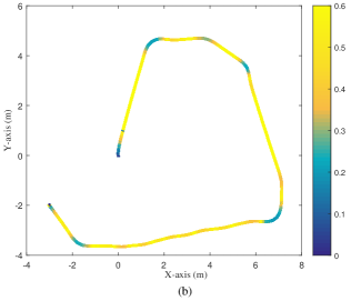
Experiments are conducted in a warehouse environment. Parameters of the proposed hierarchical controller are inherited from the simulation. Note that in our experiment setting, the actual input of the AGV dynamic model is the motor voltage rather than the torque. The dynamics of the DC motor can be approximated by a first-order inertial system with a small time constant [2]. Since the RESO-based controller is capable of handling large uncertainties and only relies on the sign of the control gain, in the implementation stage, the commands of the voltage of the DC motors are also given by (37). Fig. 11a illustrates the map of the environment and the original path generated by the A^∗ algorithm. Fig. 11b shows the MPC-improved path and the reference velocity. The maximal velocity of the AGV in the experiments is set as 0.6m/s. Figs. 12 and 13 depict the experimental results with 0 payload and 60kg payload, respectively. Note that 60kg payload is about double the weight of the AGV itself, which indicates large uncertainty corresponding to the AGV dynamics. Such uncertainty will increase the burden of the controller, and has stubborn effects on the overall control performance. However, from Figs. 12 and 13, one can observe that the AGV moves along the planned trajectory accurately, the commands generated by the MPC-based kinematic controller are well-tracked by the RESO-based dynamic controller, and the voltages of the two motors are also acceptable. Fig. 14 depicts the trajectory tracking error with 0 payload and 60kg payload. With 0 payload, the maximal tracking error is 0.071m, the average tracking error is 0.019m; with 60kg payload, the maximal tracking error is 0.105m, the average tracking error is 0.029m. The experimental video is available at https://youtu.be/SxdO9YXbiZs.

References

- [1]
- [2] C. L. Hwang, C. C. Yang, and J. Y. Hung, “Path tracking of an autonomous ground vehicle with different payloads by hierarchical improved fuzzy dynamic sliding-mode control,” IEEE Transactions on Fuzzy Systems, vol. 26, no. 2, pp. 899-914, 2018.
- [3] V. Digani, L. Sabattini, C. Secchi, and C. Fantuzzi, “Ensemble coordination approach in multi-AGV systems applied to industrial warehouses,” IEEE Transactions on Automation Science and Engineering, vol. 12, no. 3, pp. 922-934, 2015.
- [4] N. H. Amer, H. Zamzuri, K. Hudha, and Z. A. Kadir, “Modelling and control strategies in path tracking control for autonomous ground vehicles: a review of state of the art and challenges,” Journal of Intelligent and Robotic Systems, vol. 86, no. 2, pp. 225-254, 2017.
- [5] P. E. Hart, N. J. Nilsson, and B. Raphael, “A formal basis for the heuristic determination of minimum cost paths,” IEEE Transactions on Systems Science and Cybernetics, vol. 4, no. 2, pp. 100-107, 1968.
- [6] A. Stentz, “The focussed D∗ algorithm for real-time replanning,” in Proceedings of the International Joint Conference on Artificial Intelligence, 1995, pp. 1652-1659.
- [7] S. M. LaValle and J. J. Kuffner Jr, “Randomized kinodynamic planning,” The International Journal of Robotics Research, vol. 20, no. 5, pp. 378-400, 2001.
- [8] J. Villagra and D. Herrero-P´erez, “A comparison of control techniques for robust docking maneuvers of an AGV,” IEEE Transactions on Control Systems Technology, vol. 20, no. 4, pp. 1116-1123, 2012.
- [9] Y. Wu, L. Wang, J. Zhang, and L. Li, “Path following control of autonomous ground vehicle based on nonsingular terminal sliding mode and active disturbance rejection control,” IEEE Transactions on Vehicular Technology, vol. 68, no. 7, pp. 6379-6390. 2019
- [10] R. Wang, H. Jing, C. Hu, F. Yan, and N. Chen, “Robust path following control for autonomous ground vehicles with delay and data dropout,” IEEE Transactions on Intelligent Transportation Systems, vol. 17, no. 7, pp. 2042-2050, 2016.
- [11] X. Li, Z. Sun, D. Cao, D. Liu, and H. He, “Development of a new integrated local trajectory planning and tracking control framework for autonomous ground vehicles,” Mechanical Systems and Signal Processing, vol. 87, pp. 118-137, 2017.
- [12] H. Zheng, R. R. Negenborn, and G. Lodewijks, “Fast ADMM for distributed model predictive control of cooperative waterborne AGVs,” IEEE Transactions on Control Systems Technology, vol. 25, no. 4, pp. 1406-1413, 2016.
- [13] Z. Sun and Y. Xia, “Receding horizon tracking control of unicycle type robots based on virtual structure,” International Journal of Robust and Nonlinear Control, vol. 26, no. 17, pp. 3900-3918, 2016.
- [14] J. Ji, A. Khajepour, W. W. Melek, and Y. Huang, “Path planning and tracking for vehicle collision avoidance based on model predictive control with multiconstraints,” IEEE Transactions on Vehicular Technology, vol. 66, no. 2, pp. 952-964, 2016.
- [15] E. Alcalá, V. Puig, J. Quevedo, and U. Rosolia, “Autonomous racing using linear parameter varying-model predictive control (LPV-MPC),” Control Engineering Practice, vol. 95, p.104270, 2020.
- [16] S. Cheng, L. Li, X. Chen, J. Wu, and H. Wang, “Model-predictive-control-based path tracking controller of autonomous vehicle considering parametric uncertainties and velocity-varying,” IEEE Transactions on Industrial Electronics, published online, DOI: 10.1109/TIE.2020.3009585.
- [17] J. Han, “From PID to active disturbance rejection control,” IEEE Transactions on Industrial Electronics, vol. 56, no. 3, pp. 900-906, 2009.
- [18] Y. Huang and W. Xue, “Active disturbance rejection control: methodology and theoretical analysis,” ISA Transactions, vol. 53, no. 4, pp. 963-976, 2014.
- [19] E. Sariyildiz, R. Oboe, and K. Ohnishi, “Disturbance observer-based robust control and its applications: 35th anniversary overview,” IEEE Transactions on Industrial Electronics, published online, doi: 10.1109/TIE.2019.2903752.
- [20] M. Ran, Q. Wang, and C. Dong, “Active disturbance rejection control for uncertain nonaffine-in-control nonliner systems,” IEEE Transactions on Automatic Control, vol. 62, no. 11, pp. 5830-5836, 2017.
- [21] M. Ran, Q. Wang, and C. Dong, “Stabilization of a class of nonlinear systems with actuator saturation via active disturbance rejection control,” Automatica, vol. 63, pp. 302-310, 2016.
- [22] M. Ran, Q. Wang, C. Dong, and L. Xie, “Active disturbance rejection control for uncertain time-delay nonlinear systems,” Automatica, vol. 112, 108692.
- [23] J. Lee, R. Mukherjee, and H. K. Khalil, “Output feedback stabilization of inverted pendulum on a cart in the presence of uncertainties,” Automatica, vol. 54, pp. 146-157, 2015.
- [24] L. B. Freidovich and H. K. Khalil, “Performance recovery of feedback-linearization-based designs,” IEEE Transactions on Automatic Control, vol. 53, no. 10, pp. 2324-2334, 2008.
- [25] T. Jiang, C. Huang, and L. Guo, “Control of uncertain nonlinear systems based on observers and estimators,” Automatica, vol. 59, pp. 35-47, 2015.
- [26] B. Z. Guo and Z. L. Zhao, “On convergence of the nonlinear active disturbance rejection control for MIMO systems,” SIAM Journal on Control and Optimization, vol. 51, no. 2, pp. 1727-1757, 2013.
- [27] D. Wu and K. Chen, “Design and analysis of precision active disturbance rejection control for noncircular turning process,” IEEE Transactions on Industrial Electronics, vol. 56, no. 7, pp. 2746-2753, 2009
- [28] A. Wachter, “An interior point algorithm for large-scale nonlinear optimization with applications in process engineering,” Ph.D. dissertation, Carnegie Mellon University, 2003.
- [29] G. W. Recktenwald, Numerical methods with MATLAB: implementations and applications, New Jersey: Prentice Hall, 2000.
- [30] W. Xue and Y. Huang, “On frequency-domain analysis of ADRC for uncertain system,” in American Control Conference, 2013, pp. 6637-6642.
- [31] D. Fox, “KLD-sampling: Adaptive particle filters and mobile robot localization,” in Advances in Neural Information Processing Systems, pp. 26–32, 2001.