Design and Performance Analysis of a Highly Efficient Polychromatic Full-Stokes Polarization Modulator for the CRISP Imaging Spectrometer
Abstract
We present the design and performance of a polychromatic polarization modulator for the CRisp Imaging SpectroPolarimeter (CRISP) Fabry-Perot tunable narrow-band imaging spectropolarimer at the Swedish 1-m Solar Telescope (SST). We discuss the design process in depth, compare two possible modulator designs through a tolerance analysis, and investigate thermal sensitivity of the selected design. The modulator was built and has been operational since 2015. Its measured performance is close to optimal between 500 and 900 nm, and differences between the design and as-built modulator are largely understood. We show some example data, and briefly review scientific work that used data from SST/CRISP and this modulator.
1 Introduction
Our knowledge of solar magnetism relies heavily on our ability to detect and interpret the polarization signatures of magnetic fields in solar spectral lines. Consequently, new Stokes polarimeters are designed to have the capability to observe the solar atmosphere in a variety of spectral lines over a wide wavelength range. One immediate instrument requirement stemming from this need for wavelength diversity is that the polarization modulation scheme must be efficient at all wavelengths within the working range of the spectropolarimeter. (For the definition of polarimetric efficiency see del Toro Iniesta & Collados 2000.) Typically, one attempts to achieve this goal by achromatizing the polarimetric response of a modulator. This, for instance, is the rational behind the design of super-achromatic wave plates (Serkowski 1974; Samoylov et al. 2004; Ma et al. 2008). Tomczyk et al. (2010) argued that for many instruments achromaticity is too strong a constraint, and instead proposed the concept of the polychromatic modulator that is efficient at all wavelengths of interest, but has polarimetric properties that vary with wavelength.
In this paper, we present the development process of a modulator for the CRisp Imaging SpectroPolarimeter (CRISP) Fabry-Perot tunable narrow-band imaging instrument (Scharmer 2006; Scharmer et al. 2008) at the Swedish 1-m Solar Telescope (SST, Scharmer et al. 2003). First, we compare the performance of two possible modulator designs, and use a Monte-Carlo tolerance analysis to evaluate their robustness. We analyze the sensitivity of the modulator to thermal conditions, and present the opto-mechanical packaging and electrical interfaces. The modulator was constructed and tested at the High Altitude Observatory (HAO). We compare as-built properties to those of the design. Finally, we show some example polarimetric observations made using this modulator.
This modulator was designed and built to replace a modulator based on Liquid Crystal Variable Retarders (LCVRs). LCVRs are electro-optical devices that have a fixed fast axis orientation, but, as the name implies, can be set to any retardance within some range by applying an AC voltage. LCVRs generally have much slower switching speeds than Ferro-electric Liquid Crystals (). In contrast to LCVRs, have a constant retardance but switch their fast axis orientation between two states separated by a switching angle, typically around . The LCVRs in the old CRISP modulator had to be “overdriven” and the modulator state order had to be optimized in order to switch during the readout time of the CRISP cameras. More importantly, however, thermal sensitivities of the setup forced polarimetric calibration more frequently than desired (van Noort & Rouppe van der Voort 2008).
We limit ourselves to designs that use because their fast switching speed allows the state of the modulator to be changed in less than the allotted , thus allowing for the highest possible modulation rate. Fast modulation is desirable because seeing-induced crosstalk between Stokes parameters that is a dominant source of error in ground-based polarimeters is less at higher modulation rates (Lites 1987; Judge et al. 2004; Casini et al. 2012a). Also, it is of importance in maximizing the overall efficiency of the polarimeter. Many present-day CCD and CMOS detectors allow simultaneous exposure and readout that the switching speed of the modulator becomes the limitation in the overall duty cycle—and thus efficiency—of the modulator.
2 Design
A computer program was developed at HAO to determine component parameters for a given modulator design (Tomczyk et al. 2010). This program was used successfully to design the modulators for the ProMag, CoMP-S, SCD, ChroMag, and UCOMP instruments built or under construction by HAO (Elmore et al. 2008; Kučera et al. 2010; Kucera et al. 2015; de Wijn et al. 2012). More recently, it, or similar programs derived from it or independently implemented by others, have been used to design modulators, e.g., for the DKIST (Harrington & Sueoka 2018). The code can use several different merit functions. We choose to minimize the maximum of the deviation of the modulation efficiency in Stokes , , and from the optimal value of for balanced modulation at a number of user-specified wavelengths, normalized by the efficiency in Stokes .
We study two designs: one consisting of two devices followed by one fixed retarder that we will refer to as the FFR design, and one consisting of an , a fixed retarder, a second , and a second fixed retarder that we will refer to as the FRFR design. The HAO-designed instruments mentioned above all use the FFR design. Others have implemented FRFR designs (e.g., Gandorfer 1999; Keller & Solis Team 2001; Iglesias et al. 2016) The FFR design has 5 free parameters, whereas the FRFR design has 7 (see Table 1). Both have significant freedom to optimize the design over wide wavelength ranges.
All modulators discussed here were optimized for balanced modulation, i.e., equal efficiency in , , and , at 16 equidistant wavelengths over the 500—900 nm operating wavelength range of the CRISP instrument. We allow the program to choose the retardances of the and the retarders, as well as the orientations of the second and the retarders. Experience has shown that the best configurations have an orientation very close to or with respect to the orientation of the analyzing polarizer for the first . We therefore fix the orientation of the first at 0 degrees to eliminate one free parameter. The switching angle of an is sensitive to both temperature and drive voltage (Gisler 2005; Gisler et al. 2003). Hence, we assume that we can the switching angles 45 degrees. We also account for dispersion of birefingence for all elements of the modulator .
The program can use several different optimization techniques. We first use a Latin Hypercube Sampling algorithm (McKay et al. 1979) to probe the parameter space. We use a large population size of 25,000 but only 5 iterations in which we shrink the parameter space around the best solution. We then apply a downhill simplex method (Nelder & Mead 1965) to refine the solution. To increase confidence that we did not find a local minimum, we repeat the search several times and check that we consistently find the same solution. The resulting designs are summarized in Table 1.
| Component | Retardance | Orientation |
|---|---|---|
| waves at 665 nm | degrees | |
| FRFR | ||
| 1 | ||
| Retarder 1 | ||
| 2 | ||
| Retarder 2 | ||
| FFR | ||
| 1 | ||
| 2 | ||
| Retarder 1 | ||
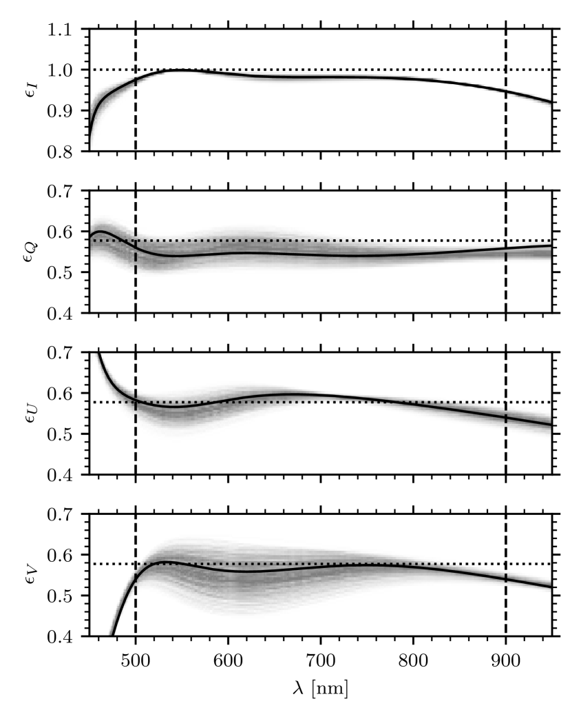
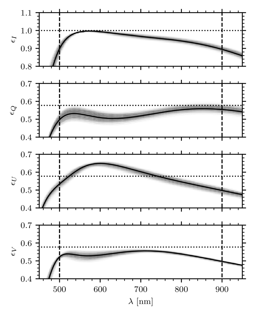
The next step is to evaluate the robustness of the design using a Monte-Carlo tolerancing method. Efficiencies were calculated for a total of 1000 modulator realizations with parameters chosen from a uniform distribution around the design values. The width of the distributions was chosen to be the vendor-supplied accuracies for the retardances of the devices of for the and for the retarder. The switching angle of the is assumed to be 45 degrees with insignificant error. typically have large manufacturing errors in their retardances. Since as-built retardances will be known prior to assembly of the modulator, the tolerancing process re-optimizes the angles of the components after the retardances have been chosen.
As an example, a realization of the FFR modulator might have with retardances of and waves, and a retarder with a value of waves, at the reference wavelength of . The tolerancing procedure would then re-optimize the modulator design to find optimal angles of and for the second and the retarder. Then, the procedure will perturb all the angles to account for mounting errors, to, say, , , and , and finally calculate the efficiencies of this modulator realization.
The resulting expected modulator performance is shown in Figs. 1 and 2. An even better result can be achieved by re-optimizing the retardances of the fixed retarders in addition to the orientations after the as-built retardances are known. This was not pursued for the CRISP modulator due to time constraints, and because the design is shown to be tolerant to expected manufacturing errors.
Figures 1 and 2 show that both designs are well-behaved. The nominal FRFR design exhibits better overall performance than the FFR design, which is not surprising in view of its higher number of degrees of freedom. The tolerance analysis shows that the FRFR design is considerably less resistant to manufacturing errors than the FFR design, particularly in between 500 and 800 nm. We show this design here to demonstrate the importance of performing a tolerance analysis. It is possible to find other FRFR designs that have slightly worse performance, but are more robust against manufacturing errors. However, the FFR design performs very well over this wavelength range and has the benefit of one less component, and thus results in a thinner stack of optics with fewer interfaces. In our case, we select the FFR design primarily because the modulator must fit in a tight space in the existing CRISP optical setup.
There is considerable freedom to pick a reference wavelength. Our experience has shown that a wavelength at or slightly below the middle of the operational range is a good choice for practical reasons. Here, we picked , also because the program chooses to use with retardances that are equal to and at that wavelength within the margin of error. We fix these components at those values and optimize the fixed retarder and component orientations. We find that the orientation of the 2nd does not change. The fixed retarder value and orientation change slightly to and .
3 Thermal Analysis
The switching angle of is somewhat sensitive to temperature. Gisler et al. (2003) measured it as a function of temperature and found a mostly linear relationship with a coefficient of .
We evaluate the effect of temperature change of the modulator following a procedure similar to Lites & Ichimoto (2013). The Stokes vector is modulated into a vector of intensities . The modulation can be described by a modulation matrix ,
| (1) |
A demodulation matrix is used to recover the Stokes vector,
| (2) |
A difference in temperature of the modulator during observations and calibrations will result in a mismatch of the modulation and demodulation matrices. We denote with derived from the calibration, and with the inferred Stokes vector,
| (3) |
We can then relate the inferred Stokes vector and the real Stokes vector through an error matrix,
| (4) |
It is easy to see that we now have
| (5) |
and using we find
| (6) |
we can calculate the modulation matrix from the unperturbed design, and demodulation matrices for several switching angles to determine the permissible change in temperature.
Limits must be imposed on every element of the matrix . The diagonal elements represent a scale error that is much less sensitive than crosstalk errors. The scaling on is unconstrained after normalizing by . Furthermore, the elements in the and columns can be scaled by the maximum expected linear polarization signal, and those in the column can be scaled by the maximum expected circular polarization signal. We follow Ichimoto et al. (2008) and adopt maxima of for the crosstalk error , for scale error, for linear polarization, and for circular polarization. We then find
| (7) |
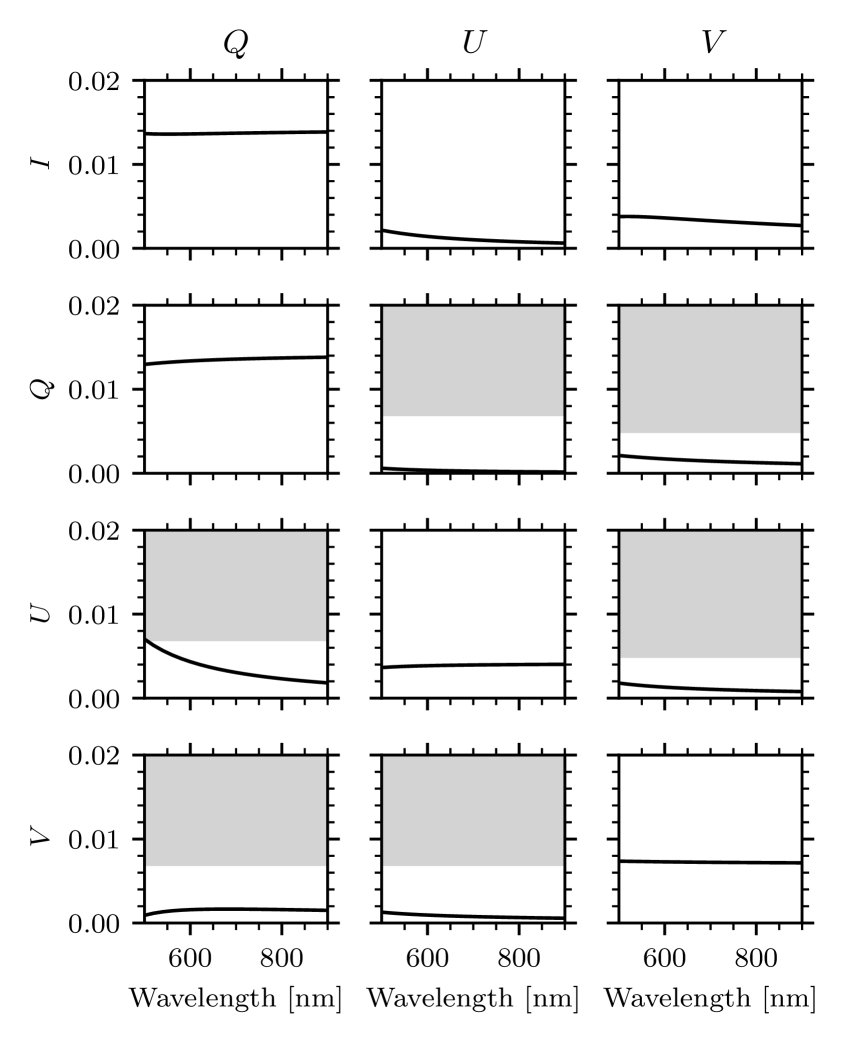
Figure 3 shows the matrix elements for the error introduced by the change in switching angle for a change in temperature. The -to- term is the worst offender and is just below the limit at .
There are other contributors to than changes in switching angle with temperature. E.g., the retardances of the and the retarder also have a small temperature dependence. The polarimetric calibration procedure also has a finite accuracy (van Noort & Rouppe van der Voort 2008). We do not explicitly model these effects here, since the switching angle is expected to be the dominant source of error. Instead we assign a fraction of the permissible error to changes in switching angle and set the requirement for thermal stability to .
4 Opto-Mechanical Design
Figure 4 shows a cross-section of the modulator. The mechanical design borrows heavily from the HAO Lyot filter designs used in the CoMP, CoMP-S, SCD, and ChroMag instruments. The modulator optics are glued into mounts that allow the optic to be oriented to any angle using a RTV silicone. The mounts consist of two parts. The inner part is round and holds the optic. It can be oriented to the desired angle and glued to the hexagonal outer part that is indexed to the inner mount assembly. The optics stack is assembled between parallel windows using index-matching gel. The windows rest on O-rings in their mounts. The entrance window mount is spring-loaded against the inner mount assembly with 4.4 N.
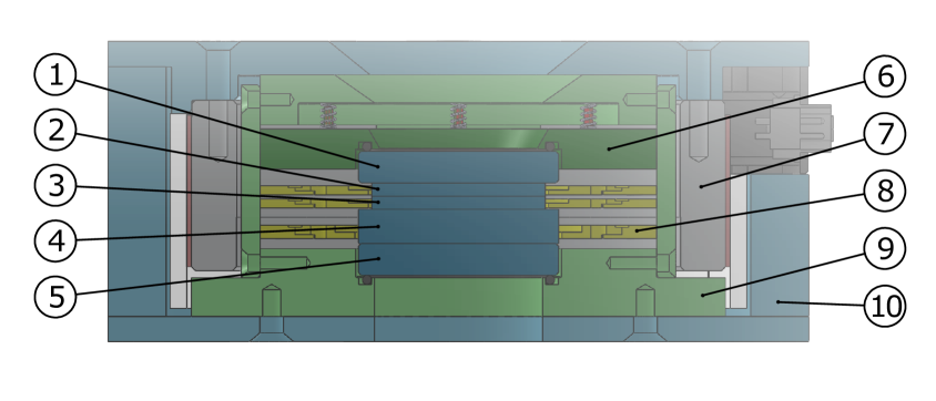
The inner mount assembly is inserted in an oven consisting of an aluminum tube with a silicone rubber heater element and aerogel insulation wrapped around it. An off-the-shelf precision temperature controller is used to stabilize the oven to to better than . The modulator is encased in a Delrin housing. Electrical connections for the and the heater system are routed to two D-subminiature connectors on the housing.
A custom controller based on an Arduino Uno microcontroller board was built to drive the . The camera software sends a voltage sequence to the controller via a serial interface, which is preloaded into two Burr-Brown DAC714 digital-to-analog converters (DACs). A synchronization pulse is then used to update the voltages when the chopper that controls the exposure of the cameras is closed. The are primarily capacitive loads, with capacitance of about . The DACs are capable of driving , which is more than adequate to drive the between states in under a millisecond. The controller also resets the voltage to zero after a few seconds of inactivity as a safety feature because the may be damaged if driven by a constant voltage for a prolonged period of time.
5 Performance
The components of the modulator must be accurately aligned to ensure proper functioning of the assembled device. HAO has a facility Lab Spectropolarimeter (LSPM) test setup for polarimetric characterization of optics that was used to test components of the CRISP modulator after they were mounted.
The LSPM consists of relay optics that feed light from a halogen bulb through, in order, a calibration package that consists of a polarizer and a retarder in individual rotation stages, the sample under test, and a polychromatic polarization modulator and analyzer, into an Ocean Optics USB4000 fiber-fed spectrograph. This setup allows for characterization of the full Mueller matrix of the sample as a function of wavelength. The spectrograph covers the wavelength range from about to about , though signal levels are low under .
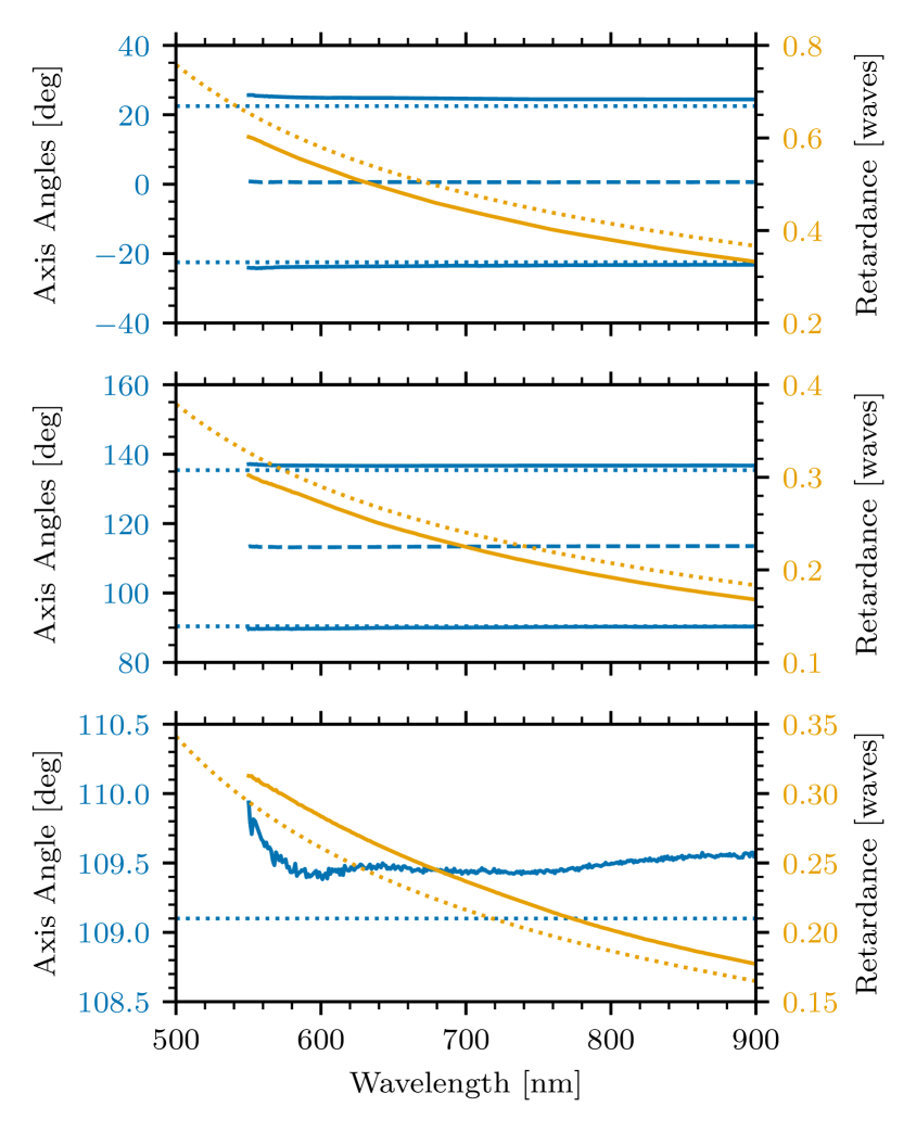
We solve for retardance and fast axis position of a linear retarder that matches the Mueller matrices derived from LSPM measurements as a function of wavelength. Figure 5 shows the results for the three CRISP modulator components. The figure also shows the design retardances and fast axis positions. The and have measured retardances of and at , The fixed retarder is measured at .
As discussed in Sect. 2, we can re-optimize the design with these values. However, we made our measurements at room temperature. The measurement should have been performed at the operating temperature of because component retardance has some temperature dependence. Using the retardance values at room temperature we find fast axis angles for the 2nd and the fixed retarder are and . However, if we assume the retarder will have its design retardance at , the fast axis positions revert to the nominal design. We choose not to change the modulator design because of the unknown effect of temperature on the component retardance and because only marginal improvement of performance is expected.
The modulator was first assembled with air gaps, and once the proper relative alignment of the components was confirmed using the LSPM, the modulator was assembled in its housing using Nye OCF-452 optical coupling fluid on the glass interfaces. The purpose of the coupling fluid is to reduce internal Fresnel reflections between the surfaces of the optics. Nye OCF-452 was used because it has a refractive index that is well-matched to the Corning XG glass of the and the BK7 glass of the retarder and windows. Internal Fresnel reflections at the optical interfaces of the components are limited to below the level.
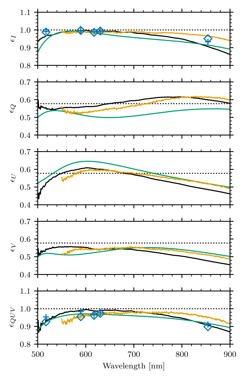
The fully assembled modulator was brought to operating temperature and tested again on the LSPM. The LSPM produces measurements of the Mueller matrix of the modulator in each of its 4 states. We simulate a perfect analyzer in to calculate modulation efficiencies, shown as a function of wavelength in Fig. 6.
The measured efficiencies largely show the expected behavior when compared to the design . However, differences in the model and measured efficiencies cannot be fully attributed to as-built retardances and component alignment. The differences are likely due to several factors that were not included in the tolerance analysis. The model assumes that the components are perfect retarders with a known dispersion of birefringence, and that the have an exact switching angle. In reality, the components have imperfections such as chromatic variation of the fast axis, and the actual dispersion of birefringence is different from the model. This can be seen in Fig. 5. The solid blue lines are not horizontal, and the solid and dotted orange lines are not parallel. The switching angle is also not exactly . Lastly, bulk rotational alignment of the modulator to the analyzer was not included in the analysis. modulator designs, in particular the traditional rotating retarder, are invariant under rotation of the modulator with respect to the analyzer. This design is not invariant, and rotation of the modulator results in depressed efficiencies.
Figure 6 also shows the modulation efficiencies computed from the Mueller matrices of the measured components . They show good agreement with the measured efficiencies of the assembled modulator. We attribute the differences mostly to the components not being measured at operating temperature. There are also likely small differences in the relative orientation of the components in the assembled modulator compared to the individual measurements.
The CRISP instrument is intended for high-resolution imaging. The modulator, therefore, must have low transmitted wavefront distortion (TWD). Because the internal optics are coupled using an index-matching gel, the TWD is dominated by the by the entrance and exit windows. Fortunately, excellent quality windows are inexpensive and commonly available. The TWD of the assembled modulator was measured using a Zygo interferometer. It was found to be at RMS over the clear aperture after removal of the tilt component, but including of power that introduces primarily a shift in focus position.
| Wavelength | |||||
|---|---|---|---|---|---|
| Transmitted | |||||
| Reflected | |||||
The modulator was installed at the SST in October 2014.
The telescope measurements include all the optics on the tables, which include a number of mirrors and lenses, a dichroic beamsplitter, the CRISP prefilter, a gray beamsplitter, and the CRISP etalons. These elements cannot be separated from the modulator. The calibration procedure fits all optics on the table between the calibration optics and the polarization analyzer as one modulation matrix (van Noort & Rouppe van der Voort 2008). In effect, all optical elements between the calibration optics and the polarimetric analyzer together act as the modulator.
The transmitted and reflected beams show very similar behavior.
The overall performance is excellent with the lowest efficiencies only slightly below (cf. the optimum and balanced efficiency of ).
6 Conclusion
The trade-offs and procedures described in this paper were employed to design the polarimetric modulator for the CRISP instrument, but can be applied to the design of modulators for other instruments. We chose to omit some steps that could result in somewhat improved performance of the modulator. If schedule permits, it is possible to incrementally optimize the design with measured optic properties. We could have delayed the purchase of the retarder until the , which have the largest errors, had been characterized at operating temperature, so that the value of the retarder could have been optimized for the as-built . While this design with only three components is robust, such incremental re-optimization may be necessary to guarantee acceptable efficiencies for modulator designs with more optical elements that cover larger wavelength ranges (Snik et al. 2012).
We did not specifically consider polarized spectral “fringes” in our design process. A description of polarized spectral fringes can be found in reviews by Lites (1991), Semel (2003), and Clarke (2004). They are interference patterns that are produced by reflections between parallel surfaces in a system with polarization optics, such as the components of the modulator, that are difficult to characterize (Harrington et al. 2017) and remove (Rojo & Harrington 2006; Casini et al. 2012b; Casini & Li 2019). Snik et al. (2015) optimized components to suppress polarized fringes for their application by ensuring that the periods of the fringes are much smaller than the spectral resolution of their instrument. the only available option Fresnel reflections from the interfaces of the optical elements. The use of optical coupling fluid is therefore not only required to address etaloning, but also to suppress these fringes.
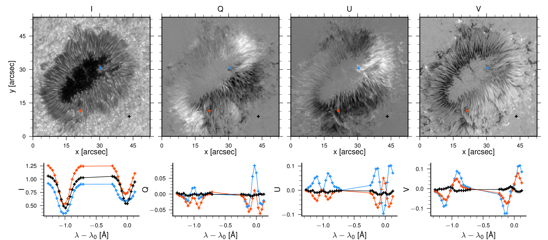
The polarimetric modulator described here has been in use for science observations at the SST starting with the 2015 observing season. Example data of a sunspot are shown in Fig. 7. The data reduction procedures are described in detail by de la Cruz Rodr´ıguez et al. (2015) and Löfdahl et al. (2018). These data can be fit using forward-modeling procedures to derive quantitative measures of atmospheric parameters, most notably the strength and direction of magnetic field. For example, Kuridze et al. (2018) studied the structure and evolution of temperature and magnetic field in a flaring active region using full-Stokes CRISP observations in the Ca II line at , Vissers et al. (2019) used similar data in combination with data from the IRIS mission (De Pontieu et al. 2014) to study Ellerman bombs and UV bursts, Vissers et al. (2020) inferred the photopheric and chromospheric magnetic field vector in a flare target and studied their differences, Libbrecht et al. (2019) used CRISP observations in the He I line in a study of a flare, Morosin et al. (2020) and Pietrow et al. (2020) studied chromospheric magnetic fields in plage targets and estimated a canopy mean field strength of in the chromosphere, and Joshi et al. (2020) studied very small-scale reconnection in the solar photosphere using CRISP polarimetry and CHROMIS (Scharmer et al. 2019) observations in H.
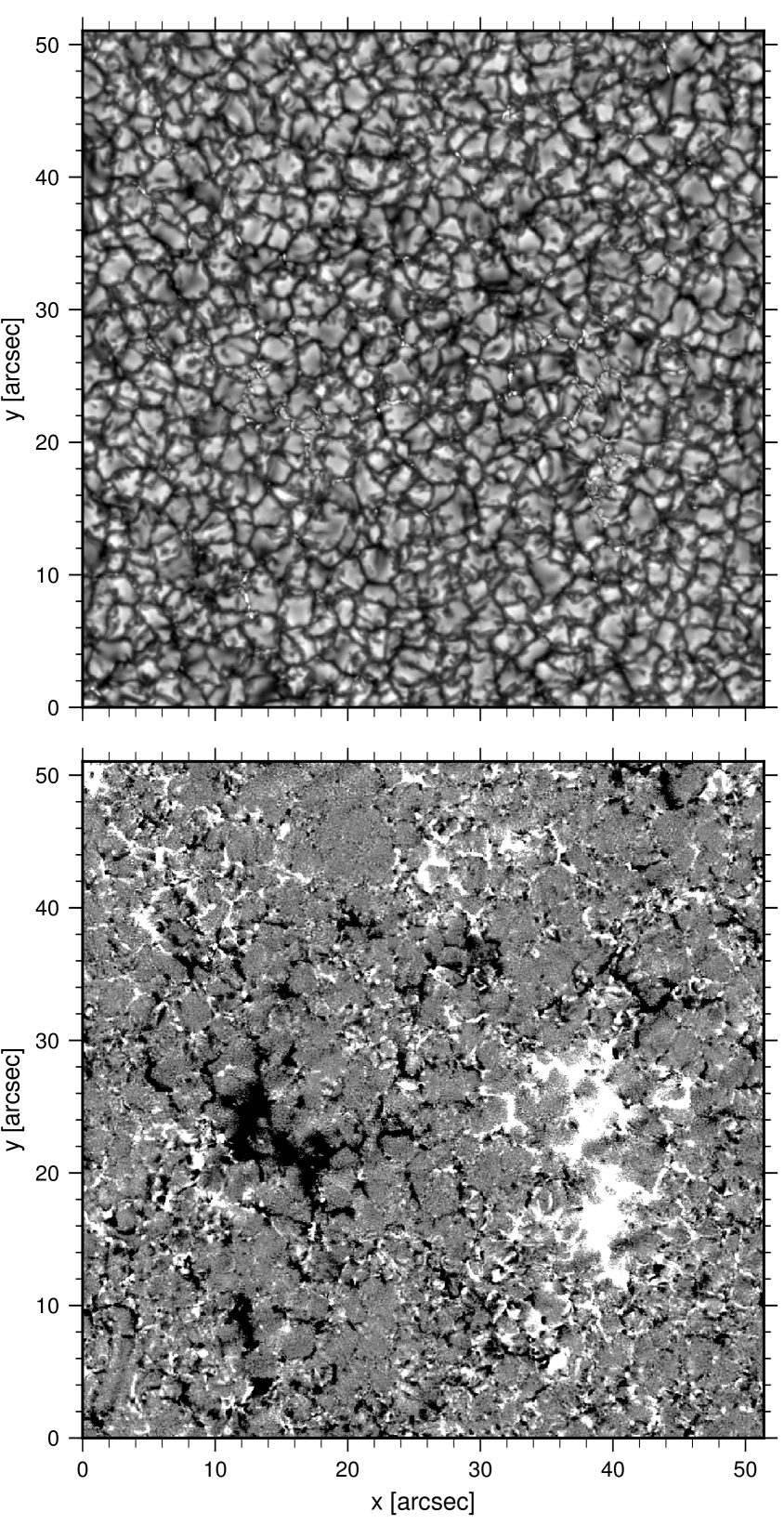
Figure 8 shows a region of quiet sun with the line-of-sight component of the magnetic field inferred from full-Stokes observations of the Fe I line profile using a spatially-regularized Milne-Eddington inversion method (de la Cruz Rodr´ıguez 2019). This example highlights the power of CRISP combined with this modulator. Quiet-sun magnetic fields are weak and difficult to detect. Telescopes and instruments that achieve high spatial resolution, have adequate spectral resolving power, and have high system efficiency are required to study them. We refer the interested reader to Bellot Rubio & Orozco Suárez (2019) for a comprehensive review of observations of quiet-sun magnetic field.
The high throughput and efficiency of CRISP with this modulator also enables observations in many lines with polarimetry while maintaining sufficient cadence for studies of dynamic events. Such multi-line observations were used by Leenaarts et al. (2018) in a study of chromospheric heating in an emerging flux region. They used the STiC code (de la Cruz Rodr´ıguez et al. 2019) to simultaneously interpret the signals from several lines. Esteban Pozuelo et al. (2019) used the same code in a similar way to study penumbral microjets.
References
- Astropy Collaboration et al. (2018) Astropy Collaboration, Price-Whelan, A. M., Sipőcz, B. M., et al. 2018, AJ, 156, 123
- Astropy Collaboration et al. (2013) Astropy Collaboration, Robitaille, T. P., Tollerud, E. J., et al. 2013, A&A, 558, A33
- Bellot Rubio & Orozco Suárez (2019) Bellot Rubio, L. & Orozco Suárez, D. 2019, Living Reviews in Solar Physics, 16, 1
- Casini et al. (2012a) Casini, R., de Wijn, A. G., & Judge, P. G. 2012a, ApJ, 757, 45
- Casini et al. (2012b) Casini, R., Judge, P. G., & Schad, T. A. 2012b, ApJ, 756, 194
- Casini & Li (2019) Casini, R. & Li, W. 2019, ApJ, 872, 173
- Clarke (2004) Clarke, D. 2004, Journal of Optics A: Pure and Applied Optics, 6, 1036
- de la Cruz Rodr´ıguez (2019) de la Cruz Rodríguez, J. 2019, A&A, 631, A153
- de la Cruz Rodr´ıguez et al. (2019) de la Cruz Rodríguez, J., Leenaarts, J., Danilovic, S., & Uitenbroek, H. 2019, A&A, 623, A74
- de la Cruz Rodr´ıguez et al. (2015) de la Cruz Rodríguez, J., Löfdahl, M. G., Sütterlin, P., Hillberg, T., & Rouppe van der Voort, L. 2015, A&A, 573, A40
- De Pontieu et al. (2014) De Pontieu, B., Title, A. M., Lemen, J. R., et al. 2014, Sol. Phys., 289, 2733
- de Wijn et al. (2012) de Wijn, A. G., Bethge, C., Tomczyk, S., & McIntosh, S. 2012, in Society of Photo-Optical Instrumentation Engineers (SPIE) Conference Series, Vol. 8446, Ground-based and Airborne Instrumentation for Astronomy IV, 844678
- del Toro Iniesta & Collados (2000) del Toro Iniesta, J. C. & Collados, M. 2000, Appl. Opt., 39, 1637
- Elmore et al. (2008) Elmore, D. F., Casini, R., Card, G. L., et al. 2008, in Society of Photo-Optical Instrumentation Engineers (SPIE) Conference Series, Vol. 7014, Ground-based and Airborne Instrumentation for Astronomy II, 701416
- Esteban Pozuelo et al. (2019) Esteban Pozuelo, S., de la Cruz Rodríguez, J., Drews, A., et al. 2019, ApJ, 870, 88
- Gandorfer (1999) Gandorfer, A. M. 1999, Optical Engineering, 38, 1402
- Gisler (2005) Gisler, D. 2005, PhD thesis, ETH Zurich
- Gisler et al. (2003) Gisler, D., Feller, A., & Gandorfer, A. M. 2003, in Society of Photo-Optical Instrumentation Engineers (SPIE) Conference Series, Vol. 4843, Proc. SPIE, ed. S. Fineschi, 45–54
- Harrington et al. (2017) Harrington, D. M., Snik, F., Keller, C. U., Sueoka, S. R., & van Harten, G. 2017, Journal of Astronomical Telescopes, Instruments, and Systems, 3, 048001
- Harrington & Sueoka (2018) Harrington, D. M. & Sueoka, S. R. 2018, Journal of Astronomical Telescopes, Instruments, and Systems, 4, 044006
- Hunter (2007) Hunter, J. D. 2007, Computing in Science and Engineering, 9, 90
- Ichimoto et al. (2008) Ichimoto, K., Lites, B., Elmore, D., et al. 2008, Sol. Phys., 249, 233
- Iglesias & Feller (2019) Iglesias, F. A. & Feller, A. 2019, Optical Engineering, 58, 082417
- Iglesias et al. (2016) Iglesias, F. A., Feller, A., Nagaraju, K., & Solanki, S. K. 2016, A&A, 590, A89
- Joshi et al. (2020) Joshi, J., Rouppe van der Voort, L. H. M., & de la Cruz Rodríguez, J. 2020, A&A, 641, L5
- Judge et al. (2004) Judge, P. G., Elmore, D. F., Lites, B. W., Keller, C. U., & Rimmele, T. 2004, Appl. Opt., 43, 3817
- Keller & Solis Team (2001) Keller, C. U. & Solis Team. 2001, in Astronomical Society of the Pacific Conference Series, Vol. 236, Advanced Solar Polarimetry – Theory, Observation, and Instrumentation, ed. M. Sigwarth, 16
- Kucera et al. (2015) Kucera, A., Tomczyk, S., Rybak, J., et al. 2015, in IAU General Assembly, Vol. 29, 2246687
- Kuridze et al. (2018) Kuridze, D., Henriques, V. M. J., Mathioudakis, M., et al. 2018, ApJ, 860, 10
- Kučera et al. (2010) Kučera, A., Ambróz, J., Gömöry, P., Kozak, M., & Rybák, J. 2010, Contributions of the Astronomical Observatory Skalnaté Pleso, 40
- Leenaarts et al. (2018) Leenaarts, J., de la Cruz Rodríguez, J., Danilovic, S., Scharmer, G., & Carlsson, M. 2018, A&A, 612, A28
- Libbrecht et al. (2019) Libbrecht, T., de la Cruz Rodríguez, J., Danilovic, S., Leenaarts, J., & Pazira, H. 2019, A&A, 621, A35
- Lites (1987) Lites, B. W. 1987, Appl. Opt., 26, 3838
- Lites (1991) Lites, B. W. 1991, in Solar Polarimetry, ed. L. J. November, 166–172
- Lites & Ichimoto (2013) Lites, B. W. & Ichimoto, K. 2013, Sol. Phys., 283, 601
- Löfdahl et al. (2018) Löfdahl, M. G., Hillberg, T., de la Cruz Rodriguez, J., et al. 2018, arXiv e-prints, arXiv:1804.03030
- Ma et al. (2008) Ma, J., Wang, J.-S., Denker, C., & Wang, H.-M. 2008, Chinese J. Astron. Astrophys., 8, 349
- McKay et al. (1979) McKay, M. D., Beckman, R. J., & Conover, W. J. 1979, Technometrics, 21, 239
- Morosin et al. (2020) Morosin, R., de la Cruz Rodriguez, J., Vissers, G. J. M., & Yadav, R. 2020, arXiv e-prints, arXiv:2006.14487
- Nelder & Mead (1965) Nelder, J. A. & Mead, R. 1965, The Computer Journal, 7, 308
- Perez & Granger (2007) Perez, F. & Granger, B. E. 2007, Computing in Science and Engineering, 9, 21
- Pietrow et al. (2020) Pietrow, A. G. M., Kiselman, D., de la Cruz Rodríguez, J., et al. 2020, arXiv e-prints, arXiv:2006.14486
- Rodenhuis et al. (2014) Rodenhuis, M., Snik, F., van Harten, G., Hoeijmakers, J., & Keller, C. U. 2014, in Society of Photo-Optical Instrumentation Engineers (SPIE) Conference Series, Vol. 9099, Polarization: Measurement, Analysis, and Remote Sensing XI, ed. D. B. Chenault & D. H. Goldstein, 90990L
- Rojo & Harrington (2006) Rojo, P. M. & Harrington, J. 2006, ApJ, 649, 553
- Samoylov et al. (2004) Samoylov, A. V., Samoylov, V. S., Vidmachenko, A. P., & Perekhod, A. V. 2004, J. Quant. Spec. Radiat. Transf., 88, 319
- Scharmer (2006) Scharmer, G. B. 2006, A&A, 447, 1111
- Scharmer et al. (2003) Scharmer, G. B., Bjelksjo, K., Korhonen, T. K., Lindberg, B., & Petterson, B. 2003, in Innovative Telescopes and Instrumentation for Solar Astrophysics, ed. S. L. Keil & S. V. Avakyan, Vol. 4853, International Society for Optics and Photonics (SPIE), 341 – 350
- Scharmer et al. (2019) Scharmer, G. B., Löfdahl, M. G., Sliepen, G., & de la Cruz Rodríguez, J. 2019, A&A, 626, A55
- Scharmer et al. (2008) Scharmer, G. B., Narayan, G., Hillberg, T., et al. 2008, ApJ, 689, L69
- Selbing (2005) Selbing, J. 2005, Master’s thesis, Stockholm Univ., arXiv:1010.4142
- Semel (2003) Semel, M. 2003, A&A, 401, 1
- Serkowski (1974) Serkowski, K. 1974, Methods of Experimental Physics, 12, 361
- Snik et al. (2015) Snik, F., van Harten, G., Alenin, A. S., Vaughn, I. J., & Tyo, J. S. 2015, in Society of Photo-Optical Instrumentation Engineers (SPIE) Conference Series, Vol. 9613, Polarization Science and Remote Sensing VII, 96130G
- Snik et al. (2012) Snik, F., van Harten, G., Navarro, R., et al. 2012, in Society of Photo-Optical Instrumentation Engineers (SPIE) Conference Series, Vol. 8446, Ground-based and Airborne Instrumentation for Astronomy IV, 844625
- Tomczyk et al. (2010) Tomczyk, S., Casini, R., de Wijn, A. G., & Nelson, P. G. 2010, Appl. Opt., 49, 3580
- van der Walt et al. (2011) van der Walt, S., Colbert, S. C., & Varoquaux, G. 2011, Computing in Science and Engineering, 13, 22
- van Noort & Rouppe van der Voort (2008) van Noort, M. J. & Rouppe van der Voort, L. H. M. 2008, A&A, 489, 429
- Vissers et al. (2020) Vissers, G. J. M., Danilovic, S., de la Cruz Rodriguez, J., et al. 2020, arXiv e-prints, arXiv:2009.01537
- Vissers et al. (2019) Vissers, G. J. M., de la Cruz Rodríguez, J., Libbrecht, T., et al. 2019, A&A, 627, A101