Details of a Hybrid Model for the Interaction between the Solar Wind and Planets Implemented in FLASH

In the hybrid approximation, ions are treated as particles, and electrons as a massless fluid. In what follows we use SI units. The trajectory of an ion, $\mathbf{r}(t)$ and $\mathbf{v}(t)$, with charge $q$ and mass $m$, is computed from the Lorentz force,

$$\frac{\displaystyle d\mathbf{r}}{\displaystyle dt}=\mathbf{v},\quad\frac{\displaystyle d\mathbf{v}}{\displaystyle dt}=\frac{\displaystyle q}{\displaystyle m}\left(\mathbf{E}+\mathbf{v}\times\mathbf{B}\right),$$

where $\mathbf{E}=\mathbf{E}(\mathbf{r},t)$ is the electric field, and $\mathbf{B}=\mathbf{B}(\mathbf{r},t)$ is the magnetic field. From now on we do not write out the dependence on $\mathbf{r}$ and $t$. The electric field is given by

$$\mathbf{E}=\frac{\displaystyle 1}{\displaystyle\rho_{I}}\left(-\mathbf{J}_{I}\times\mathbf{B}+\mu_{0}^{-1}\left(\nabla\times\mathbf{B}\right)\times\mathbf{B}-\nabla p_{e}\right)+\frac{\eta}{\mu_{0}}\nabla\times\mathbf{B},$$

(1)

where $\rho_{I}$ is the ion charge density, $\mathbf{J}_{I}$ is the ion current density, $p_{e}$ is the electron pressure, $\eta$ is the resistivity, and $\mu_{0}=4\pi\cdot 10^{-7}$ is the magnetic constant. Then Faraday’s law is used to advance the magnetic field in time,

$$\frac{\displaystyle\partial\mathbf{B}}{\displaystyle\partial t}=-\nabla\times\mathbf{E}.$$

Note that the unknowns are the position and velocity of the ions, and the magnetic field on a grid, not the electric field, since it can always be computed from (1). As is common for hybrid models, we use the Darwin approximation (Schmitz and Grauer, 2006), i.e. we neglect the displacement current in Ampere’s law, and the current then is $\mathbf{J}=\mu_{0}^{-1}\nabla\times\mathbf{B}$. This removes waves that propagate with the speed of light, $c$. For the problems we study the velocities are small compared to $c$ and the transport of energy by electromagnetic radiation can be neglected. This makes the approximation reasonable for our purposes. If the Darwin approximation is not used we would have the severe restriction on the time step of $\Delta t<\Delta x/c$.

We have implemented a parallel hybrid solver in the FLASH open source software framework (Fryxell et al., 2000). Further details on the hybrid model used here, and the discretization, can be found in Holmström (2011a, b, 2013). The solver has been applied to studies of the interaction between the solar wind and planets, e.g., the Moon (Holmström et al., 2012).

In the following sections we present some details of this hybrid model. How we handle permanent magnetic fields, how ionospheric chemistry for Mars can be included in the model, and some analytical expressions for Mars’ exosphere.

In many applications there is a background magnetic field that does not change over time. An example can be the internal dipole field of a planet, or the solar wind magnetic field. For simplicity and accuracy over long time runs we can split the field into a time varying part and a constant in time part (Tanaka, 1995). We can then solve for $\mathbf{B}(\mathbf{r},t)=\mathbf{B}_{0}(\mathbf{r})+\Delta\mathbf{B}(\mathbf{r},t)$. Note that $\Delta\mathbf{B}$ does not need to be small. To ensure that $\nabla\cdot\mathbf{B}=0$ we can define $\mathbf{B}_{0}(\mathbf{r})=-\nabla\psi(\mathbf{r})$, then we also have that $\nabla\times\mathbf{B}_{0}=0$. Inserting this into the hybrid equations, we find that $\mathbf{B}_{0}$ then only appears in the Lorentz force and in the first term of the electric field expression. All other terms in the electric field expression involving $\mathbf{B}_{0}$ are zero since $\mathbf{B}_{0}$ is rotation free.

To implement this in the hybrid solver it is important that $\nabla\cdot\mathbf{B}_{0}=0$ also in the discrete sense. This can be ensured by computing the background field from the potential, $\mathbf{B}_{0}(\mathbf{r})=-\nabla\psi(\mathbf{r})$ using the same finite difference approximation of the gradient that we use for the divergence. In our case we use the same centered finite difference stencil. This ensures that the discrete $\nabla\cdot\mathbf{B}_{0}=0$ down to round-off errors. Note that $\mathbf{B}_{0}$ need only be computed once, at the start of the simulation, and stored.

As an example, the potential for a dipole is

$$\psi(\mathbf{r})=\frac{\mu_{0}}{4\pi}\frac{\mathbf{m}\cdot\mathbf{r}}{r^{3}}=\frac{\mathbf{m}\cdot\mathbf{r}}{r^{3}}\cdot 10^{-7}\mbox{ [T m].}$$

Then

$$\mathbf{B}_{d}=-\nabla\psi(\mathbf{r})=\frac{\mu_{0}}{4\pi r^{3}}\left(3\frac{\mathbf{r}\left(\mathbf{m}\cdot\mathbf{r}\right)}{r^{2}}-\mathbf{m}\right)=\frac{10^{-7}}{r^{3}}\left(3\frac{\mathbf{r}\left(\mathbf{m}\cdot\mathbf{r}\right)}{r^{2}}-\mathbf{m}\right).$$

Here $\mathbf{m}$ is the dipole moment [T m³]. The background field from a dipole located at $\mathbf{r}_{c}$ then is $\mathbf{B}_{0}(\mathbf{r})=\mathbf{B}_{d}(\mathbf{r}-\mathbf{r}_{c})$.

For a conducting sphere of radius $R$ in a uniform field $\mathbf{B}_{u}$, currents in the sphere will expel the external field such that the component normal to the sphere surface is zero. The resulting total field outside the sphere can be seen as the sum of the external field and a dipole at the center of the sphere directed opposite to the external field. The magnitude of the required dipole moment is $m=10^{7}R^{3}B_{u}/2$.

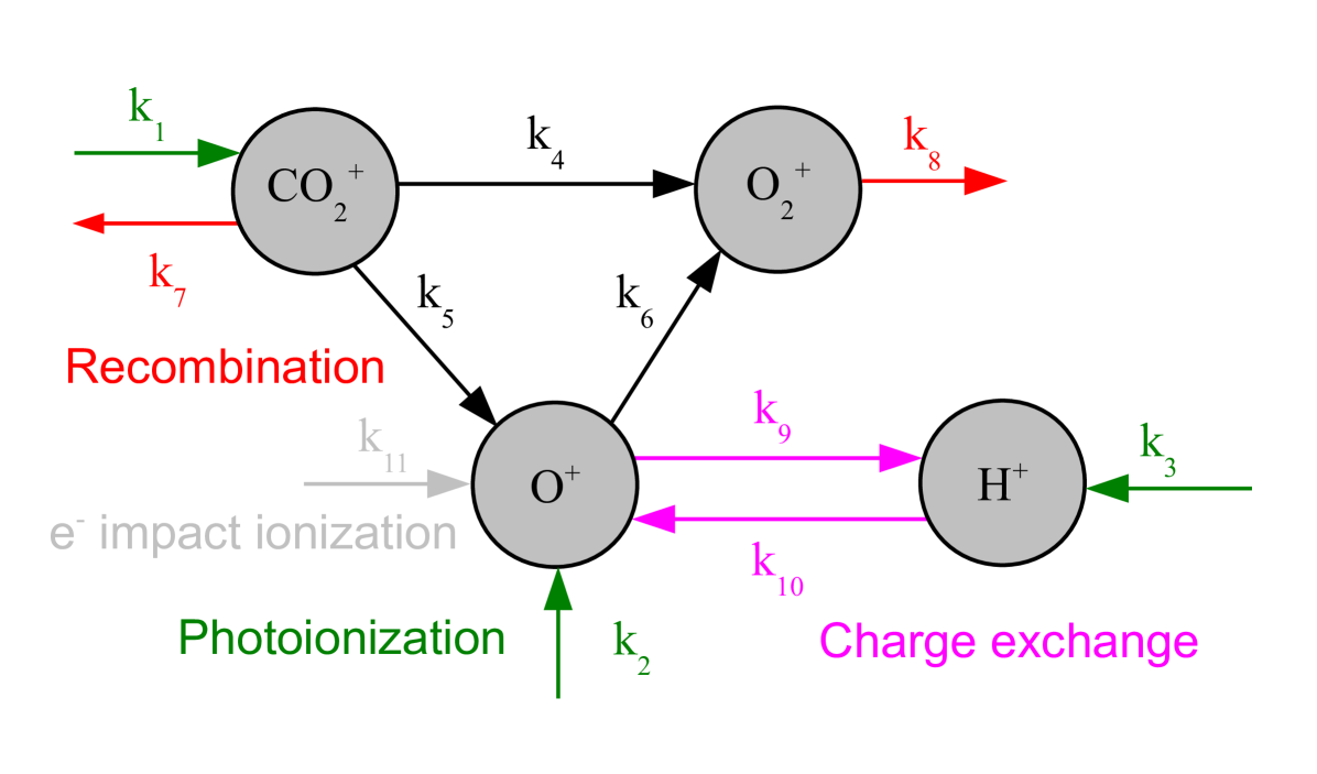
For Mars ionosphere one can consider only the major ion species CO${}_{2}^{+}$, O⁺, and O${}_{2}^{+}$. A table of the most relevant chemical reactions involving these species was presented by Ma et al. (2004). A similar table is provided by Brecht and Ledvina (2012), with the addition of oxygen electron impact ionization, e+O $\rightarrow$ O⁺+e+e. The different reactions are presented in Figure 1 and in Table 1. We also consider the hydrogen exosphere, but H only occur for photoionization and charge exchange.

We can note that all reactions depend only on one ion species, so we can adopt a Monte Carlo approach where for each meta-ion we can compute the probability that it undergo a reaction and then randomly convert it to another ion. Recombination reactions also depend on the electron density (total charge density) so we have to get that value from the grid.

The initial ion densities are important. We disregard charge exchange for initial distributions.

Here square brackets denote number density of a species, e.g., $[A]$ m^-3 for a species $A$. We consider the density of neutrals as constant in radial background profiles

$$[\textrm{H}](r),[\textrm{O}](r),[\textrm{CO}_{2}](r)$$

where the density only depends on distance, $r$, from the center of Mars. So the neutral atmosphere is an unchanging source and sink. This is an acceptable approximation at Mars to large distances from the planet since the neutral densities are so much larger than the ion densities.

The unknowns here are the ion number densities as a function of position and time

$$[\textrm{H}^{+}](\mathbf{r},t),[\textrm{O}^{+}](\mathbf{r},t),[\textrm{O}_{2}^{+}](\mathbf{r},t),[\textrm{CO}_{2}^{+}](\mathbf{r},t).$$

We will also need the electron number density

$$[e](\mathbf{r},t)=[\textrm{H}^{+}]+[\textrm{O}^{+}]+[\textrm{O}_{2}^{+}]+[\textrm{CO}_{2}^{+}].$$

Using the reactions in Ma et al. (2004) we can then write the evolution of ion number densities at each position $\mathbf{r}$ (no transport is considered) as

	$\displaystyle\frac{\displaystyle d}{\displaystyle dt}[\textrm{H}^{+}]$	$\displaystyle=$	$\displaystyle k_{3}[\textrm{H}]+k_{9}[\textrm{H}][\textrm{O}^{+}]-k_{10}[\textrm{O}][\textrm{H}^{+}]$
	$\displaystyle\frac{\displaystyle d}{\displaystyle dt}[\textrm{O}^{+}]$	$\displaystyle=$	$\displaystyle k_{2}[\textrm{O}]+k_{5}[\textrm{O}][\textrm{CO}_{2}^{+}]-k_{6}[\textrm{CO}_{2}][\textrm{O}^{+}]-k_{9}[\textrm{H}][\textrm{O}^{+}]+k_{10}[\textrm{O}][\textrm{H}^{+}]+k_{11}[\textrm{O}][\textrm{e}]$
	$\displaystyle\frac{\displaystyle d}{\displaystyle dt}[\textrm{CO}_{2}^{+}]$	$\displaystyle=$	$\displaystyle k_{1}[\textrm{CO}_{2}]-(k_{4}+k_{5})[\textrm{O}][\textrm{CO}_{2}^{+}]-k_{7}[\textrm{CO}_{2}^{+}][\textrm{e}]$
	$\displaystyle\frac{\displaystyle d}{\displaystyle dt}[\textrm{O}_{2}^{+}]$	$\displaystyle=$	$\displaystyle k_{4}[\textrm{O}][\textrm{CO}_{2}^{+}]+k_{6}[\textrm{CO}_{2}][\textrm{O}^{+}]-k_{8}[\textrm{O}_{2}^{+}][\textrm{e}]$

Some of the constants $k_{i}$ also depend on ion and electron temperature, $T_{i}$ and $T_{e}$. We list the coefficients in Table 1. All coefficients except for $k_{11}$ come from Krasnopolsky (2002). The coefficient $k_{11}$ is re-cited from Roberson et al. (2007).

The chemistry can be implemented using a Monte Carlo approach. Each existing ion in the simulation has an average time for each reaction. If we denote such a time $\tau$, after each time step, for each meta-particle, we draw a random time from an exponential distribution with mean $\tau$. The event occur if this time is smaller than the time step. For photoionization these times are listed in Table 1. The times for the other reactions are listed in Table 2.

At the beginning of the simulation we could start with no ionospheric ions and let them evolve over time using the Monte Carlo approach. It could however take too long time to reach a steady state. We could instead initialize the ionospheric densities in our simulation model to values close to the steady state. Exact values are not needed since ion transport will anyway change the state over time. Then we need to compute the steady state number densities of ions. This can be done by integration in time until a steady state is reached Brecht and Ledvina (2012). Alternatively, setting the time derivatives to zero above gives us a system of non-linear equations, the solution of which is the steady state solution. The equations are non-linear due to the presence of the electron density in the equations. It is not possible to compute a simple analytical solution to the above equations. It is however possible to find the solution numerically. This is similar to using an implicit in time solver to compute the steady state solution.

There are very few measurements of the hydrogen exosphere of Mars, all of which are UV remote sensing experiments (Anderson and Hord, 1971; Anderson, 1974, 1976; Chaufray et al., 2008; Feldman et al., 2011). Among these experiments, most observations were been done with the Lyman-$\alpha$ line except for the Rosetta/ALICE observation (Feldman et al., 2011), that employed the Lyman-$\beta$ line as well. Although the Lyman-$\alpha$ emission is the strongest ($\approx 250$ times stronger than that of Lyman-$\beta$), it is not optically thin below 10000 km altitude (Anderson, 1976; Feldman et al., 2011), meaning that one has to model the radiative transfer processes in the hydrogen exosphere to resolve the density profile, and the result is usually not unique. The density profiles resolved from Lyman-$\alpha$ observations consist of two components: a cold or thermal population with a temperature of $\approx 200$ K at the exobase, consistent with Chamberlain’s theory of exosphere formation, and a hot or supra-/non thermal population with a temperature of more than 500 K at the exobase, the production mechanism of which is yet unclear. The Lyman-$\beta$ line, on the other hand, is optically thin except for the lowest altitudes at the planetary limb. This allows to interpret the emission intensity by the simple integration along the line of sight therefore the density profile is better constrained. The altitude profiles derived by the Lyman-$\beta$ observation does not include the hot population. In our current study we take the one from the Lyman-$\beta$ line observation by Rosetta/ALICE due to its more straightforward physics and less peculiarity.

We have presented the implementation of several model details for a parallel hybrid solver in the FLASH open source software framework. First, an inclusion of permanent magnetic fields such that the divergence of the magnetic field is ensured to be zero in the discrete sense was presented. Secondly, a Monte Carlo algorithm for including ionospheric chemistry in the model is introduced, along with reaction times from the existing literature. Finally, an analytical fit for Mars hydrogen and oxygen exosphere, based on Rosetta observations, is presented.

This research was conducted using resources provided by the Swedish National Infrastructure for Computing (SNIC) at the High Performance Computing Center North (HPC2N), Umeå University, Sweden. The software used in this work was in part developed by the DOE NNSA-ASC OASCR Flash Center at the University of Chicago.

References

- Anderson and Hord (1971) Anderson, D. E. and Hord, C. W. 1971, Journal of Geophysical Research, 76, 6666
- Anderson (1974) Anderson, D. E. 1974, Journal of Geophysical Research, 79, 1513
- Anderson (1976) Anderson, D. E. 1976, Journal of Geophysical Research, 81, 1213
- Brecht and Ledvina (2012) Brecht, S. H. and Ledvina, S. A. 2012, Earth Planets Space, 64, 165
- Chaufray et al. (2008) Chaufray, J. Y., et al. 2008, Icarus, 195, 598
- Feldman et al. (2011) Feldman, P. D., et al. 2011, Icarus, 214, 394
- Fryxell et al. (2000) Fryxell, B., et al. 2000, The Astrophysical Journal Supplement Series, 131, 273
- Harned (1982) Harned, D. S. 1982, Journal of Computational Physics, 47, 452
- Hewett (1980) Hewett, D. W. 1980, Journal of Computational Physics, 38, 378
- Holmström (2011a) Holmström, M. 2011a, in Proceedings of ENUMATH 2009 (Springer), 451. ArXiv:0911.4435
- Holmström (2011b) Holmström, M. 2011b, in Numerical modeling of space plasma flows (ASTRONUM-2010), ASP conference series, 444, 211 ArXiv:1010.3291
- Holmström et al. (2012) Holmström, M., et al. 2012, Earth Planets Space, 64, 237
- Holmström (2013) Holmström, M. 2013, in Numerical modeling of space plasma flows (ASTRONUM-2012), ASP conference series, 474, 202 ArXiv:1010.3291
- Krasnopolsky (2002) Krasnopolsky, V. A. 2002, Journal of Geophysical Research, 107, E12, 11
- Ma et al. (2004) Ma, Y., et al. 2004, Journal of Geophysical Research, 109, A07211
- Roberson et al. (2007) Roberson, G., et al. 2007, Brazilian Journal of Physics, 37, 457
- Schmitz and Grauer (2006) Schmitz, H., and Grauer, R., 2006, Journal of Computational Physics, 214, 2, 738
- Tanaka (1995) Tanaka, T. 1995, Journal of Geophysical Research, 100, A7, 12057