∎
[]crCorresponding author \thankstexte1e-mail: 2802368240@qq.com \thankstexte2e-mail: 924038358@qq.com \thankstexte3e-mail: yangjichong@lnnu.edu.cn
Detect anomalous quartic gauge couplings at muon colliders with quantum kernel k-means
Abstract
In recent years, with the increasing luminosities of colliders, handling the growing amount of data has become a major challenge for future New Physics (NP) phenomenological research. In order to improve efficiency, machine learning algorithms have been introduced into the field of high-energy physics. As a machine learning algorithm, kernel k-means has been demonstrated to be useful for searching NP signals. It is well known that the kernel k-means algorithm can be carried out with the help of quantum computing, which suggests that quantum kernel k-means (QKKM) is also a potential tool for NP phenomenological studies in the future. This paper investigates how to search for NP signals using QKKM. Taking the process at a muon collider as an example, the dimension-8 operators contributing to anomalous quartic gauge couplings (aQGCs) are studied. The expected coefficient constraints obtained using the QKKM of three different forms of quantum kernels, as well as the constraints obtained by the classical k-means algorithm are presented, and it can be shown that QKKM can help to find the signal of aQGCs. Comparing the classical k-means anomaly detection algorithm with QKKM, it is indicated that the QKKM is able to archive a better cut efficiency.
1 Introduction
Significant developments have been made in the field of quantum computing. The development of quantum computers has progressed from theoretical models to practical applications, with quantum processors now capable of performing complex calculations at significantly faster speeds than their classical counterparts. Researchers are continuing to advance the frontiers of quantum computing, resulting in groundbreaking developments in hardware, algorithms, and applications Arute:2019zxq . The capacity to process vast quantities of data at hitherto unattainable speeds renders quantum computing a potentially transformative force across a multitude of disciplines.
Meanwhile, as the large hadron collider (LHC) experiment enters the post-Higgs discovery era, physicists have begun to work on the search for new physics (NP) beyond the Standard Model (SM) Ellis:2012zz . The search for NP has now become one of the frontiers of high-energy physics (HEP), who frequently entails the examination of extensive datasets, generated by means of particle collisions or other experimental procedures. The potential for quantum computing to significantly accelerate data processing and analysis makes it an invaluable tool for advancing the detection of NP signals. Despite quantum computing is still in the era of noisy intermediate-scale quantum (NISQ) devices Preskill:2018jim ; Arute:2019zxq ; CG2023 , its applications in various aspects of HEP has already been discussed Zhu:2024own ; Carena:2022kpg ; Bauer:2022hpo ; Roggero:2018hrn ; Roggero:2019myu ; Gustafson:2022xdt ; Lamm:2024jnl ; Carena:2024dzu ; Atas:2021ext ; Li:2023vwx ; Cui:2019sfz ; Zou:2021pvl ; Georgescu:2013oza ; Lamm:2019uyc ; Li:2021kcs ; Echevarria:2020wct ; Jordan:2011ci ; Mueller:2019qqj ; Chou:2023hcc ; Bauer:2019qxa .
In the phenomenological studies of NP, the SM Effective Field Theory (SMEFT) is frequently used in recent years. The SMEFT framework extends the SM to incorporate high-dimensional operators that capture potential NP effects Weinberg:1979sa ; Grzadkowski:2010es ; Brivio:2017vri ; Buchmuller:1985jz . Research on SMEFT has focused on dimension-6 operators, however, from a phenomenological point of view, the dominant effect in many cases occurs in dimension-8 operators Ellis:2018cos ; Ellis:2019zex ; Ellis:2020ljj ; Gounaris:2000dn ; Gounaris:1999kf ; Senol:2018cks ; Fu:2021mub ; Degrande:2013kka ; Jahedi:2022duc ; Jahedi:2023myu ; Ellis:2017edi ; Gounaris:1999kf . In addition, dimension-8 operators are also important for convex geometric perspective operator spaces Bi:2019phv ; Zhang:2020jyn ; Yamashita:2020gtt . As a result, the dimension-8 operators are increasingly being focused on. For one generation of fermions, there are different baryon number conserving dimension-8 operators. It is necessary to conduct a detailed kinematic analysis of each of these operators. As the number of operators to be considered increases, the efficiency of the process tends to decline.
In order to facilitate the efficient analysis of data, anomaly detection (AD) machine learning (ML) algorithms have been employed in previous studies within the field of HEP to search for NP signals Zhang:2023khv ; Zhang:2023ykh ; Dong:2023nir ; Zhang:2023yfg ; Yang:2022fhw ; Yang:2021kyy ; Jiang:2021ytz ; Vaslin:2023lig ; Kuusela:2011aa ; Collins:2018epr ; Atkinson:2022uzb ; Kasieczka:2021xcg ; Farina:2018fyg ; Cerri:2018anq ; vanBeekveld:2020txa ; CrispimRomao:2020ucc ; Ren:2017ymm ; Abdughani:2018wrw ; Ren:2019xhp . This paper investigates the application of a quantum ML (QML) algorithm to search for NP, i.e., quantum kernel k-means (QKKM). The choice of the k-means algorithm among various ML algorithms is motivated by two factors. Firstly, it has been demonstrated to be effective in phenomenological studies of NP Zhang:2023yfg . Secondly, the kernel k-means algorithm is compatible with quantum computers. One potential advantage of QKKM is that, it is pointed out that multi-state swap test on quantum computers can compute inner products of multiple vectors simultaneously Liu:2022jsp ; Fanizza:2020qjq . At the same time, quantum kernels have the potential to transform nonlinear data into linearly separable forms through quantum feature mapping Liu:2020lhd . This paper aims to compare several different quantum kernel methods, all of which are inner products and have the potential to be accelerated by multi-state swap test.
In this paper, we take the study of dimension-8 operators contributing to anomalous quartic gauge couplings (aQGCs) as an example. The sensitivity of the vector boson scattering (VBS) process to aQGCs and the increasing phenomenological research on aQGCs have led to a wide interest in aQGCs Green:2016trm ; Chang:2013aya ; Anders:2018oin ; Zhang:2018shp ; Bi:2019phv ; Guo:2020lim ; Guo:2019agy ; Yang:2021pcf ; Yang:2020rjt . Meanwhile, LHC has been closely following the aQGCs ATLAS:2014jzl ; CMS:2020gfh ; ATLAS:2017vqm ; CMS:2017rin ; CMS:2020ioi ; CMS:2016gct ; CMS:2017zmo ; CMS:2018ccg ; ATLAS:2018mxa ; CMS:2019uys ; CMS:2016rtz ; CMS:2017fhs ; CMS:2019qfk ; CMS:2020ypo ; CMS:2020fqz . With the increasing luminosities on future colliders, the muon colliders can achieve higher energies and luminosities while providing a cleaner experimental environment that is less impacted by the QCD background than the hadron colliders Buttazzo:2018qqp ; Delahaye:2019omf ; Costantini:2020stv ; Lu:2020dkx ; AlAli:2021let ; Franceschini:2021aqd ; Palmer:1996gs ; Holmes:2012aei ; Liu:2021jyc ; Liu:2021akf . In order to study aQGCs, the process at muon colliders is used as a testbed. This process not only lends itself to the study of aQGCs, a NP operator of widely interest, but also provides a place to validate ML algorithms due to the information lost by final-state neutrinos. The AD event selection strategy with QKKM is employed to search for aQGCs signals, and expected coefficient constraints, i.e. the projected sensitivities are analyzed. It is worth noting that, as an AD algorithm, using the QKKM to search for aQGCs signals does not depend on the studied process.
The rest of the paper is organized as follows. In Section 2, a brief introduction to aQGCs and the process is given. The event selection strategy of QKKM is discussed in Section 3. Section 4 presents numerical results for the expected coefficient constraints. Section 5 is a summary of the conclusions.
2 aQGCs and the process of at the muon colliders
The frequently used dimension-8 operators contributing to aQGCs can be classified into three categories, scalarlongitudinal operators , mixed transverse and longitudinal operators and transverse operators , respectively Eboli:2006wa ; Eboli:2016kko . The operators involved in the process are and ,
| (1) |
where and are dimensionless Wilson coefficients, and is the NP energy scale. The process of at the muon collider can be contributed by the operators and , where are not considered due to sensitivities within current coefficient constraints and,
| (2) | ||||
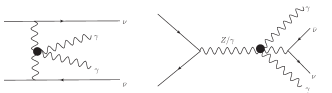
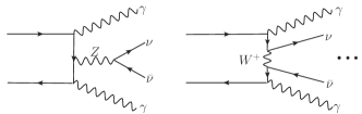
where with being the Pauli matrices and , and are and gauge fields, and correspond to the field strength tensors, and is the covariant derivative. For the process , the diagrams induced by and operators are shown in the Fig. 1, and the Fig. 2 shows the typical diagrams in the SM. Since aQGC decouple from anomalous triple gauge couplings (aTGCs) starting from dimension-8, we consider only dimension-8 operators.
As a high-energy collider, the muon collider is also considered a gauge boson collider and is therefore well suited to the study of aQGCs. The operators that contribute independently to aQGCs and are not related to anomalous triple gauge couplings start at dimension-. The muon collider is therefore well suited to study the signal of the dimension-8 aQGCs in the VBS processes. Among the many VBS processes, those in which the forward-moving particles are neutrinos have an advantage because there is no need to detect charged particles near the direction of the beams. These are processes that contain sub-processes. Among these processes, the one in which the final state are photons has the least electroweak vertices and is therefore more advantageous, which is the process that is the focus of this work. Since there are no indications of higher-dimensional operators yet, we restrict ourselves to focusing only on the projected sensitivities of the aQGCs, ignoring the effects of other SMEFT operators.
As an Effective Field Theory (EFT), the SMEFT is only valid under the NP energy scale. The high center-of-mass (c.m.) energy achievable at muon colliders offers an excellent opportunity to detect potential NP signals, while at the same time, raises concerns on the validity of the SMEFT. Previous studies have extensively employed partial wave unitarity as a criterion for assessing the validity of the SMEFT Dong:2023nir ; Yang:2021pcf ; Guo:2020lim ; Yue:2021snv ; Fu:2021mub ; Yang:2022ilt ; Layssac:1993vfp ; Corbett:2017qgl ; Almeida:2020ylr ; Kilian:2018bhs ; Kilian:2021whd ; Perez:2018kav . For the process with and correspond to the helicities of the vector bosons, in the c.m. frame with z-axis along the flight direction of in the initial state, the amplitudes can be expanded as Jacob:1959at ,
| (3) | ||||
where and are zenith and azimuth angles of , , and is the Wigner D-functions. The partial wave unitarity bound is Corbett:2014ora .
In Refs. Guo:2019agy ; Yang:2021ukg , the results of partial wave unitarity bounds on coefficients of the vertices have been obtained in the study of VBS process at the LHC. The dimension-8 operators contribute to five different vertices, with each vertex being contributed to by only one operator. Consequently, the partial wave unitarity bounds on coefficients of the vertices can be directly translated to the partial wave unitarity bounds on operator coefficients for the by assuming one operator at a time. The strongest partial wave unitarity bounds w.r.t. the process are,
| (4) |
| 10 TeV | 14 TeV | |
|---|---|---|
The maximum possible c.m. energy for the subprocess is identical to the c.m. energy of the process . At muon colliders, we consider two cases of the expected energies, and Palmer:1996gs , the tightest unitarity bounds are listed in Table 1.
K-means AD algorithm can be utilized to address interference Zhang:2023yfg . However, in this paper, due to the limited computational resources, we do not consider the interference terms for simplicity. The contribution of the SM (denoted as ), the NP (denoted as where is the name of operator), and the interference between the SM and NP (denoted as ) for different operators when the coefficients are the upper bounds in Table 1 at and are listed in Table 2. We only study operators where the cross-sectional ratio of the interference term to the NP contribution is less than (for , is at ). That is, we focus on the operators and .
The smaller the coefficient, the more important the interference terms are. From Table 1, it can be seen that the unitarity bounds are not yet at a level where the interference terms become dominant. Dimensional analysis indicates that and , when , . At , the rough estimation is that, the interference terms become important when . From the numerical results that follow, the interference term can be ignored in the following sections. This is mainly due to the fact that the constraints on are not small enough. Moreover, we mainly consider the operators, where the dominant contributions come from the scattering of the transversely polarized , which is different from the the case of the SM where the contribution of scattering of longitudinally polarized dominants, and thus the interference terms are suppressed.
The relative contributions of the VBS processes to the annihilation process are contingent upon the specific process under consideration Chen:2022yiu ; Han:2024gan , particularly in scenarios where the interference term is important. For the process , a comparison of the contributions of the VBS and tri-boson induced by when the interference term is not considered is provided in Ref. Yang:2020rjt . In this case, the VBS contribution exceeds that of the tri-boson at approximately . For the operators, the contributions are presented in the A. The tri-boson contribution is at the next order of compared to the VBS. Consequently, it can be expected that at a smaller compared with , the VBS contribution will dominant. This also explains the focus on the operators in this study, since the annihilation processes usually have larger interferences Chen:2022yiu ; Han:2024gan ; Yang:2020rjt which is ignored.
3 The event selection strategy of QKKM
As the luminosities of future colliders continue to increase, so does the quantity of data that must be processed which presents a significant challenge to conventional computing. Nevertheless, forecasts by IBM, Google, and IonQ indicate that within the next decade, it will become feasible to execute practical computational tasks using quantum computers with thousands of qubits. This coincides with the high luminosity upgrade of the LHC Apollinari:2015wtw and future colliders such as muon colliders. In recent years, numerous QML algorithms have been the subject of study within the field of HEP, such as QSVM, quantum variational classifiers etc Guan:2020bdl ; Wu:2021xsj ; Wu:2020cye ; Terashi:2020wfi ; Zhang:2023ykh
The inherent properties of coherence and entanglement in quantum systems endow quantum computers with powerful parallel computing capabilities. The main motivation for this study lies in its potential future applications. In contrast to classical computers, quantum computers are capable of storing and processing a greater quantity of data simultaneously. It is conceivable that in the future, the data that must be processed may originate directly from quantum computers. In addition, quantum computer can implement kernel functions that are difficult to achieve with classical computers Havlicek:2018nqz ; Liu:2020lhd ; Sherstov:2020qax . In this section, we use the QKKM to verify its feasibility in searching for NP.
3.1 Data preparation
In order to investigate the QKKM, the events are generated using coefficients that correspond to the upper bounds of the partial wave unitarity constraints.
The Monte Carlo (MC) simulation is performed using the MadGraph5@NLO toolkit Alloul:2013bka ; Alwall:2014hca ; Christensen:2008py ; Degrande:2011ua , while the muon collider-like detector simulation is conducted with the Delphes deFavereau:2013fsa software.
The analysis of the signals and the background is performed with the MLAnalysis MLAnalysis .
To avoid infrared divergences, we use the basic cut as the default setting.
The cut relevant to infrared divergences are,
| (5) |
where and are the transverse momentum and pseudo-rapidity for each photon, respectively, where and are differences between the azimuth angles and pseudo-rapidities of two photons. The signal events for are generated with one operator at a time.
| observables | ||||||
|---|---|---|---|---|---|---|
| observables |
In order to collect the features, we require that the final state contains at least two photons (which is denoted as cut). At a lepton collider, conservation of momentum can be employed to ascertain the full set of missing momentum components. In this paper, we choose the components of the four-momenta of the two hardest photons (the hardest photon is denoted as and the second hardest photon is denoted as , respectively) and the missing momentum. These observables form a 12-dimensional vector denoted by , of which the components are listed in Table 3.
Before training, the dataset is standardized by using z-score standardization Donoho_2004 ,
| (6) |
where and represent the mean value and standard deviation of the -th feature over the SM training datasets. The values of and at different c.m. energies are listed in Tables 4 and 5, respectively.
3.2 Using QKKM to search for aQGCs
In this paper, kernel k-means algorithm is used to replace the k-means algorithm. The number of clusters in the kernel k-means is denoted as . The steps to implement QKKM are shown as follows Zhang:2023yfg ,
-
1.
Use the quantum circuits to calculate the kernel matrices.
-
2.
Compute the centroids of the clusters by substituting the precomputed kernel matrices into the
tslearnpackage JMLR:v21:20-091 . -
3.
Repeat steps 2 for times.
-
4.
Calculate the anomaly score for each point, i.e., the distance (denoted by ) from the point to the centroid with the same value (cluster assignment) as the point.
-
5.
Calculate the average anomaly score (denoted by ) over iterations.
-
6.
Use as a cut to select the events.
The only difference between this paper and Ref. Zhang:2023yfg is that the calculation of kernel matrix is implemented using a quantum circuit.
| kernel | single qubit gate | CNOT gate |
|---|---|---|
| real vector kernel | ||
| complex vector kernel | ||
| hardware-efficient kernel |
Due to limited computational resources, the 5000 SM events are selected for training. To map the vector to a quantum state, we use both real and complex vector mapping, i.e., the quantum state presenting the event is denoted as,
| (7) |
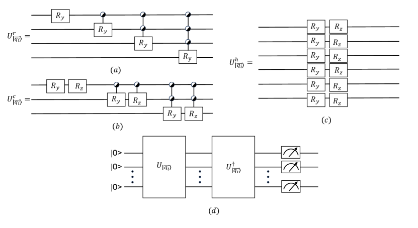
where is the digital representing of a state, is the -th component of defined in Eq. (6), and . Using Eq. (7), the length of is also encoded. An qubit state can encode a vector with degrees of freedom. Using Eq. (7), a complex vector can be encoded using three qubits, and a real vector can be encoded using four qubits. In this paper, we use amplitude encode which is denoted as , such that . The amplitude encode of Eq. (7) is implemented with the help of uniform rotation gates and Mottonen:2004vly as shown in Fig. 3. (a) and (b). Apart from Eq. (6), we also try the hardware-efficient encoding Wu:2020cye ; Fadol:2022umw ; Havlicek:2018nqz ; Bravo-Prieto:2019kld ; Kandala:2017vok ; Park:2024rim . The hardware-efficient encoding usually consists of multiple layers. Each layer consists of single qubit gates with the variables as degrees to be rotated, and the layers are separated by CNOT or controlled-Z gates connecting different qubits. The hardware-efficient encoding is difficult to be implemented using classical computers. Since there are only variables, a single layer is sufficient, necessitating the use of qubits, as shown in Fig. 3. (c). The swap test can only calculate the absolute value of the inner product, therefore one cannot distinguish between inner product results of and . To overcome this limitation, five cases are tested, i.e., we assign the angles to be rotated as , , , and , and yields the best performance. In the following, only the results with are shown. The number of gates used in the three types of encodings are listed in Table 6.
To calculate the centroids, the distance needs to be defined, which is,
| (8) |
where is the kernel function.
The kernel function is , which can be calculated using a circuit shown in Fig. 3. (d).
The probability of the outcome in the measurements is in the circuit shown in Fig. 3. (d).
The calculation of the kernel matrix is implemented using QuEST Jones:2019knd .
The measurement is repeated for times for each inner product.
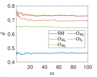
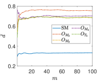
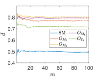
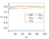
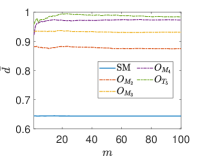
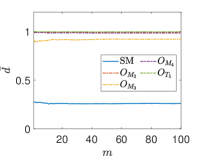
Due to the random nature of the k-means algorithm, the results of the centroids are not unique. To circumvent this issue, the process is repeated times, where is a tunable parameter. At and , one event is selected from the SM background and and signals, respectively, and is shown as a function of at in Fig. 4. We found that rapidly converges with increasing , and when , the value of begins to stabilize. Theoretically, the value of can be further increased to reduce the relative statistical error of . However, due to limited computational power, we use in this paper.
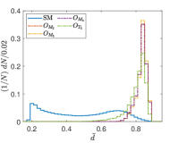
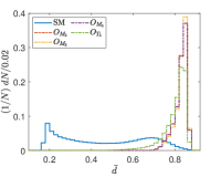
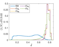
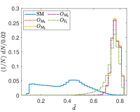
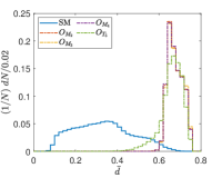
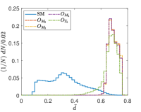
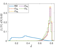
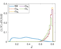
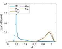
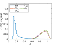
Another tunable parameter is . In general, an increase in the value of leads to an improvement in the sampling of the background event distribution, as evidenced in reference Zhang:2023yfg . However, this comes at the cost of greater computational resources being required. Accordingly, an appropriate value of is selected to achieve an optimal balance between accuracy and computational efficiency. Fig. 5 shows the normalized distributions of anomaly scores for the SM and NP events under different values in the case of complex vector kernel. It is evident that the anomaly score distributions for the SM background and NP events are more distinct with larger . The value of is set to for all kernels in this study. The resulting normalized distributions of the real vector kernel and the hardware-efficient kernel are shown in Fig. 6. From the Figs. 5 and 6, it can be seen that the distributions of for the SM background and the NP signals are different, the of the SM events are generally less than those of the NP events. From Fig. 6, it can also be observed that while hardware-efficient kernel shows good discrimination between the SM and NP, there is a small tail for the SM events residuals within the NP region.
4 expected coefficient constraints on the coefficients
| Operator | |||
| SM | |||
| Operator | |||
| SM | |||
Ignoring the interference between the SM and the aQGCs, the cross-section after cut can be expressed as,
| (9) |
where and are cross-sections of the SM and NP contributions, respectively. The NP contribution is the one when , where is the operator coefficient, and is the upper bounds of partial wave unitarity bounds listed in Table 1. and are the cut efficiencies of the cut, and are the cut efficiencies of the QKKM event selection strategy. Numerical results of and are listed in Table 2. , are listed in Table 7.
The expected coefficient constraints after cuts can be estimated by the signal significance defined as,
| (10) |
where are the event numbers of the signal and background, and , and is the luminosity. The integrated luminosities in both “conservative” and “optimistic” cases Black:2022cth ; Accettura:2023ked are considered.
| kernel | ||
|---|---|---|
| real vector kernel | ||
| complex vector kernel | ||
| hardware-efficient kernel | ||
| classical kernel |
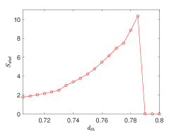
To maximize signal significance, an appropriate threshold value is selected.
Taking the real vector kernel operator at as an example.
As shown in Fig. 7, varies with within the given range.
The corresponding value is chosen as the final threshold when reaches its maximum.
The shape of the function in other scenarios is similar to that shown in Fig. 7.
The results of for the real vector kernel, the complex vector kernel, and the hardware-efficient kernel are listed in Table 8.
To compare the results of quantum and classical algorithm, the classical kernel is included.
The expected coefficient constraints are calculated using the classical kernel from the scikit-learn Pedregosa:2011ork package, following the same steps as in Ref. Zhang:2023yfg .
The for the classical kernel is also listed in Table 8.
In quantum computing, since the kernel is computed using inner products, the value of always lies between and , which is not the case for the classical k-means where the definition of is different which is the Euclidean distance Zhang:2023yfg .
| real vector kernel | ||
|---|---|---|
| Operator | () | () |
| SM | ||
| complex vector kernel | ||
| Operator | () | () |
| SM | ||
| hardware-efficient kernel | ||
| Operator | () | () |
| SM | ||
| classical kernel | ||
| Operator | () | () |
| SM | ||
The and are defined as the cut efficiencies of QKKM event selection strategy. The cut efficiencies of the four different kernels when the are chosen as the ones listed in Table 8 are listed in Table 9. As can be seen from Table 9, for the complex vector kernel, a relatively strict is taken, which is due to the fact that the background can be suppressed to a very low level. For hardware-efficient kernel, a relatively loose is taken due to the fact that the tail of the background events in the NP region. All the s are chosen according to .
| 10 TeV | 14 TeV | 14 TeV | ||
| 3 | ||||
| 10 TeV | 14 TeV | 14 TeV | ||
| 2 | ||||
| 3 | ||||
| 5 | ||||
| 2 | ||||
| 3 | ||||
| 5 | ||||
| 2 | ||||
| 3 | ||||
| 5 | ||||
| 2 | ||||
| 3 | ||||
| 5 |
| 10 TeV | 14 TeV | 14 TeV | ||
| 2 | ||||
| 3 | ||||
| 5 | ||||
| 2 | ||||
| 3 | ||||
| 5 | ||||
| 2 | ||||
| 3 | ||||
| 5 | ||||
| 2 | ||||
| 3 | ||||
| 5 |
| 10 TeV | 14 TeV | 14 TeV | ||
| 2 | ||||
| 3 | ||||
| 5 | ||||
| 2 | ||||
| 3 | ||||
| 5 | ||||
| 2 | ||||
| 3 | ||||
| 5 | ||||
| 2 | ||||
| 3 | ||||
| 5 |
| coefficient | ||||
|---|---|---|---|---|
| constraint |
When is chosen, the expected coefficient constraints can be obtained by using signal significance. The results of the expected coefficient constraints in the case of complex vector kernel, real vector kernel, hard-efficient kernel, and the classical kernel are shown in Tables 10, 11, 12, and 13, respectively. It can be seen that the muon collider with has tighter constraints than the ones at the LHC CMS:2019qfk ; CMS:2020ypo in Table 14. We speculate that this is due to the fact that, compared to the classical case, the Hilbert space in which the data resides is of higher dimensionality and thus the data is better separable. The sensitivities of the muon colliders to the aQGCs are competitive with future hadron colliders and even better at the same c.m. energy. The muon colliders are suitable to study the aQGCs because of the high energies and luminosities as well as having a cleaner experimental environment than hadron colliders.
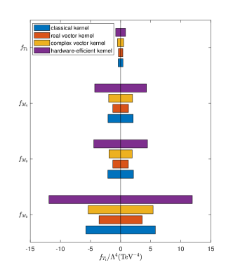
For comparison, we take and as an example, as can be seen from the Fig. 8, the expected coefficient constraints are tightest for coefficients and when the kernel is real vector kernel. This shows that instead of affecting the performance of k-means, the quantum kernel function outperforms a classical kernel. While the SM and NP signals are most effectively distinguished when utilizing the hardware-efficient kernel, the fact that the SM leaves small residuals in the NP signals results in the least stringent constraints.
After all, it can be conclude that the QKKM algorithm is an effective tool to search for the NP signals. The real vector kernel works better than the classical kernel, not to mention the potential that the QKKM can cope with future developments in quantum computing for example when the MC data is generated by a quantum computer. Note that for all the quantum kernels, the matrix elements can be calculated using swap test, therefore can be accelerated by multi-state swap test Liu:2022jsp ; Fanizza:2020qjq .
At this stage, the effect of noise in quantum computing is unavoidable. In comparison with the Ref. Zhang:2023ykh , the quantum computer has the same task of computing the kernel matrix, two of the quantum kernel functions (real and complex vector kernels) used are the same, the dimensions of the vectors dealt with are of the same order of magnitude, and thus the number of qubits used is the same, and the size of the datasets are also of the same order of magnitude. Therefore, we directly borrow the results from the Ref. Zhang:2023ykh to estimate the effect of noise. According to Ref. Zhang:2023ykh , the noise-induced relative errors when using the real and complex vector kernels can be estimated to be about . In addition, the error from noise induced by the hardware-efficient kernel is expected to be even smaller, because the quantum circuit of the hardware-efficient kernel does not contain CNOT gates. Therefore, the above error value is the upper limit of the noise-induced error of the hardware-efficient kernel.
5 Summary
The search for new physics (NP) signals requires the processing of large volumes of data, and quantum computing has the potential to accelerate these computations in the future. This paper focuses on the process at a muon collider, a process highly sensitive to dimension-8 operators involved in anomalous quartic gauge couplings (aQGCs). We use kernel K-means AD to search for the signals of the NP. In this paper, three different types of quantum kernels and a classical kernel are used.
The results indicate that this process is indeed highly sensitive to the aQGCs. The kernel K-means AD algorithm, utilizing the three distinct quantum kernels (when a quantum kernel is used, it is QKKM), as well as the classical kernel-based algorithm, proved feasible for NP signal searches. Compared to the LHC, the muon collider offers more stringent coefficient constraints. Among the four kernels, the real vector kernel demonstrated the best performance. Therefore, it is suggested that the QKKM is well suited for the phenomenological study of the NP, especially when progress in quantum computing are anticipated.
Acknowledgements.
This work was supported in part by the National Natural Science Foundation of China under Grants No. 12147214, the Natural Science Foundation of the Liaoning Scientific Committee Nos. LJKZ0978 and LJKMZ20221431.Appendix A Contributions of tri-boson and VBS processes for operators
Contributions of tri-boson and VBS processes for operator is established in Ref. Yang:2020rjt . For operators, using effective vector boson approximation Kane:1984bb ; Boos:1997gw ; Ruiz:2021tdt , at the leading order of ,
| (11) |
with . For the tri-boson case, at the leading order of ,
| (12) |
References
- (1) F. Arute, et al., Quantum supremacy using a programmable superconducting processor, Nature 574 (7779) (2019) 505–510. arXiv:1910.11333, doi:10.1038/s41586-019-1666-5.
- (2) J. Ellis, Outstanding questions: Physics beyond the Standard Model, Phil. Trans. Roy. Soc. Lond. A 370 (2012) 818–830. doi:10.1098/rsta.2011.0452.
- (3) J. Preskill, Quantum Computing in the NISQ era and beyond, Quantum 2 (2018) 79. arXiv:1801.00862, doi:10.22331/q-2018-08-06-79.
-
(4)
C. Gill,
5
year update to the next steps in quantum computing workshop, Computing
Community Consortium (2023).
URL https://cra.org/ccc/events/5-year-update-to-the-next-steps-in-quantum-computing-workshop/ - (5) Y. Zhu, W. Zhuang, C. Qian, Y. Ma, D. E. Liu, M. Ruan, C. Zhou, A Novel Quantum Realization of Jet Clustering in High-Energy Physics Experiments, 2024. arXiv:2407.09056.
- (6) M. Carena, H. Lamm, Y.-Y. Li, W. Liu, Improved Hamiltonians for Quantum Simulations of Gauge Theories, Phys. Rev. Lett. 129 (5) (2022) 051601. arXiv:2203.02823, doi:10.1103/PhysRevLett.129.051601.
- (7) C. W. Bauer, et al., Quantum Simulation for High-Energy Physics, PRX Quantum 4 (2) (2023) 027001. arXiv:2204.03381, doi:10.1103/PRXQuantum.4.027001.
- (8) A. Roggero, J. Carlson, Dynamic linear response quantum algorithm, Phys. Rev. C 100 (3) (2019) 034610. arXiv:1804.01505, doi:10.1103/PhysRevC.100.034610.
- (9) A. Roggero, A. C. Y. Li, J. Carlson, R. Gupta, G. N. Perdue, Quantum Computing for Neutrino-Nucleus Scattering, Phys. Rev. D 101 (7) (2020) 074038. arXiv:1911.06368, doi:10.1103/PhysRevD.101.074038.
- (10) E. J. Gustafson, H. Lamm, F. Lovelace, D. Musk, Primitive quantum gates for an SU(2) discrete subgroup: Binary tetrahedral, Phys. Rev. D 106 (11) (2022) 114501. arXiv:2208.12309, doi:10.1103/PhysRevD.106.114501.
- (11) H. Lamm, Y.-Y. Li, J. Shu, Y.-L. Wang, B. Xu, Block encodings of discrete subgroups on a quantum computer, Phys. Rev. D 110 (5) (2024) 054505. arXiv:2405.12890, doi:10.1103/PhysRevD.110.054505.
- (12) M. Carena, H. Lamm, Y.-Y. Li, W. Liu, Quantum error thresholds for gauge-redundant digitizations of lattice field theories, Phys. Rev. D 110 (5) (2024) 054516. arXiv:2402.16780, doi:10.1103/PhysRevD.110.054516.
- (13) Y. Y. Atas, J. Zhang, R. Lewis, A. Jahanpour, J. F. Haase, C. A. Muschik, SU(2) hadrons on a quantum computer via a variational approach, Nature Commun. 12 (1) (2021) 6499. arXiv:2102.08920, doi:10.1038/s41467-021-26825-4.
- (14) Y.-Y. Li, M. O. Sajid, J. Unmuth-Yockey, Lattice holography on a quantum computer, Phys. Rev. D 110 (3) (2024) 034507. arXiv:2312.10544, doi:10.1103/PhysRevD.110.034507.
- (15) X. Cui, Y. Shi, J.-C. Yang, Circuit-based digital adiabatic quantum simulation and pseudoquantum simulation as new approaches to lattice gauge theory, JHEP 08 (2020) 160. arXiv:1910.08020, doi:10.1007/JHEP08(2020)160.
- (16) Y.-T. Zou, Y.-J. Bo, J.-C. Yang, Optimize quantum simulation using a force-gradient integrator, EPL 135 (2021) 10004. arXiv:2103.05876, doi:10.1209/0295-5075/135/10004.
- (17) I. M. Georgescu, S. Ashhab, F. Nori, Quantum Simulation, Rev. Mod. Phys. 86 (2014) 153. arXiv:1308.6253, doi:10.1103/RevModPhys.86.153.
- (18) H. Lamm, S. Lawrence, Y. Yamauchi, Parton physics on a quantum computer, Phys. Rev. Res. 2 (1) (2020) 013272. arXiv:1908.10439, doi:10.1103/PhysRevResearch.2.013272.
- (19) T. Li, X. Guo, W. K. Lai, X. Liu, E. Wang, H. Xing, D.-B. Zhang, S.-L. Zhu, Partonic collinear structure by quantum computing, Phys. Rev. D 105 (11) (2022) L111502. arXiv:2106.03865, doi:10.1103/PhysRevD.105.L111502.
- (20) M. G. Echevarria, I. L. Egusquiza, E. Rico, G. Schnell, Quantum simulation of light-front parton correlators, Phys. Rev. D 104 (1) (2021) 014512. arXiv:2011.01275, doi:10.1103/PhysRevD.104.014512.
- (21) S. P. Jordan, K. S. M. Lee, J. Preskill, Quantum Computation of Scattering in Scalar Quantum Field Theories, Quant. Inf. Comput. 14 (2014) 1014–1080. arXiv:1112.4833.
- (22) N. Mueller, A. Tarasov, R. Venugopalan, Deeply inelastic scattering structure functions on a hybrid quantum computer, Phys. Rev. D 102 (1) (2020) 016007. arXiv:1908.07051, doi:10.1103/PhysRevD.102.016007.
- (23) A. Chou, et al., Quantum Sensors for High Energy Physics, 2023. arXiv:2311.01930.
- (24) C. W. Bauer, W. A. de Jong, B. Nachman, D. Provasoli, Quantum Algorithm for High Energy Physics Simulations, Phys. Rev. Lett. 126 (6) (2021) 062001. arXiv:1904.03196, doi:10.1103/PhysRevLett.126.062001.
- (25) S. Weinberg, Baryon and Lepton Nonconserving Processes, Phys. Rev. Lett. 43 (1979) 1566–1570. doi:10.1103/PhysRevLett.43.1566.
- (26) B. Grzadkowski, M. Iskrzynski, M. Misiak, J. Rosiek, Dimension-Six Terms in the Standard Model Lagrangian, JHEP 10 (2010) 085. arXiv:1008.4884, doi:10.1007/JHEP10(2010)085.
- (27) I. Brivio, M. Trott, The Standard Model as an Effective Field Theory, Phys. Rept. 793 (2019) 1–98. arXiv:1706.08945, doi:10.1016/j.physrep.2018.11.002.
- (28) W. Buchmuller, D. Wyler, Effective Lagrangian Analysis of New Interactions and Flavor Conservation, Nucl. Phys. B 268 (1986) 621–653. doi:10.1016/0550-3213(86)90262-2.
- (29) J. Ellis, S.-F. Ge, Constraining Gluonic Quartic Gauge Coupling Operators with gg→, Phys. Rev. Lett. 121 (4) (2018) 041801. arXiv:1802.02416, doi:10.1103/PhysRevLett.121.041801.
- (30) J. Ellis, S.-F. Ge, H.-J. He, R.-Q. Xiao, Probing the scale of new physics in the coupling at colliders, Chin. Phys. C 44 (6) (2020) 063106. arXiv:1902.06631, doi:10.1088/1674-1137/44/6/063106.
- (31) J. Ellis, H.-J. He, R.-Q. Xiao, Probing new physics in dimension-8 neutral gauge couplings at e+e- colliders, Sci. China Phys. Mech. Astron. 64 (2) (2021) 221062. arXiv:2008.04298, doi:10.1007/s11433-020-1617-3.
- (32) G. J. Gounaris, J. Layssac, F. M. Renard, Off-shell structure of the anomalous and selfcouplings, Phys. Rev. D 62 (2000) 073012. arXiv:hep-ph/0005269, doi:10.1103/PhysRevD.65.017302.
- (33) G. J. Gounaris, J. Layssac, F. M. Renard, Signatures of the anomalous and production at the lepton and hadron colliders, Phys. Rev. D 61 (2000) 073013. arXiv:hep-ph/9910395, doi:10.1103/PhysRevD.61.073013.
- (34) A. Senol, H. Denizli, A. Yilmaz, I. Turk Cakir, K. Y. Oyulmaz, O. Karadeniz, O. Cakir, Probing the Effects of Dimension-eight Operators Describing Anomalous Neutral Triple Gauge Boson Interactions at FCC-hh, Nucl. Phys. B 935 (2018) 365–376. arXiv:1805.03475, doi:10.1016/j.nuclphysb.2018.08.018.
- (35) Q. Fu, J.-C. Yang, C.-X. Yue, Y.-C. Guo, The study of neutral triple gauge couplings in the process e+e→Z including unitarity bounds, Nucl. Phys. B 972 (2021) 115543. arXiv:2102.03623, doi:10.1016/j.nuclphysb.2021.115543.
- (36) C. Degrande, A basis of dimension-eight operators for anomalous neutral triple gauge boson interactions, JHEP 02 (2014) 101. arXiv:1308.6323, doi:10.1007/JHEP02(2014)101.
- (37) S. Jahedi, J. Lahiri, Probing anomalous ZZ and Z couplings at the e+e- colliders using optimal observable technique, JHEP 04 (2023) 085. arXiv:2212.05121, doi:10.1007/JHEP04(2023)085.
- (38) S. Jahedi, Optimal estimation of dimension-8 neutral triple gauge couplings at the e+e- colliders, JHEP 12 (2023) 031. arXiv:2305.11266, doi:10.1007/JHEP12(2023)031.
- (39) J. Ellis, N. E. Mavromatos, T. You, Light-by-Light Scattering Constraint on Born-Infeld Theory, Phys. Rev. Lett. 118 (26) (2017) 261802. arXiv:1703.08450, doi:10.1103/PhysRevLett.118.261802.
- (40) Q. Bi, C. Zhang, S.-Y. Zhou, Positivity constraints on aQGC: carving out the physical parameter space, JHEP 06 (2019) 137. arXiv:1902.08977, doi:10.1007/JHEP06(2019)137.
- (41) C. Zhang, S.-Y. Zhou, Convex Geometry Perspective on the (Standard Model) Effective Field Theory Space, Phys. Rev. Lett. 125 (20) (2020) 201601. arXiv:2005.03047, doi:10.1103/PhysRevLett.125.201601.
- (42) K. Yamashita, C. Zhang, S.-Y. Zhou, Elastic positivity vs extremal positivity bounds in SMEFT: a case study in transversal electroweak gauge-boson scatterings, JHEP 01 (2021) 095. arXiv:2009.04490, doi:10.1007/JHEP01(2021)095.
- (43) Y.-T. Zhang, X.-T. Wang, J.-C. Yang, Searching for gluon quartic gauge couplings at muon colliders using the autoencoder, Phys. Rev. D 109 (9) (2024) 095028. arXiv:2311.16627, doi:10.1103/PhysRevD.109.095028.
- (44) S. Zhang, Y.-C. Guo, J.-C. Yang, Optimize the event selection strategy to study the anomalous quartic gauge couplings at muon colliders using the support vector machine and quantum support vector machine, Eur. Phys. J. C 84 (8) (2024) 833. arXiv:2311.15280, doi:10.1140/epjc/s10052-024-13208-4.
- (45) Y.-F. Dong, Y.-C. Mao, i.-C. Yang, J.-C. Yang, Searching for anomalous quartic gauge couplings at muon colliders using principal component analysis, Eur. Phys. J. C 83 (7) (2023) 555. arXiv:2304.01505, doi:10.1140/epjc/s10052-023-11719-0.
- (46) S. Zhang, J.-C. Yang, Y.-C. Guo, Using k-means assistant event selection strategy to study anomalous quartic gauge couplings at muon colliders, Eur. Phys. J. C 84 (2) (2024) 142. arXiv:2302.01274, doi:10.1140/epjc/s10052-024-12494-2.
- (47) J.-C. Yang, X.-Y. Han, Z.-B. Qin, T. Li, Y.-C. Guo, Measuring the anomalous quartic gauge couplings in the W+W→W+W process at muon collider using artificial neural networks, JHEP 09 (2022) 074. arXiv:2204.10034, doi:10.1007/JHEP09(2022)074.
- (48) J.-C. Yang, Y.-C. Guo, L.-H. Cai, Using a nested anomaly detection machine learning algorithm to study the neutral triple gauge couplings at an e+e collider, Nucl. Phys. B 977 (2022) 115735. arXiv:2111.10543, doi:10.1016/j.nuclphysb.2022.115735.
- (49) L. Jiang, Y.-C. Guo, J.-C. Yang, Detecting anomalous quartic gauge couplings using the isolation forest machine learning algorithm, Phys. Rev. D 104 (3) (2021) 035021. arXiv:2103.03151, doi:10.1103/PhysRevD.104.035021.
- (50) L. Vaslin, V. Barra, J. Donini, GAN-AE: an anomaly detection algorithm for New Physics search in LHC data, Eur. Phys. J. C 83 (11) (2023) 1008. arXiv:2305.15179, doi:10.1140/epjc/s10052-023-12169-4.
- (51) M. Kuusela, T. Vatanen, E. Malmi, T. Raiko, T. Aaltonen, Y. Nagai, Semi-Supervised Anomaly Detection - Towards Model-Independent Searches of New Physics, J. Phys. Conf. Ser. 368 (2012) 012032. arXiv:1112.3329, doi:10.1088/1742-6596/368/1/012032.
- (52) J. H. Collins, K. Howe, B. Nachman, Anomaly Detection for Resonant New Physics with Machine Learning, Phys. Rev. Lett. 121 (24) (2018) 241803. arXiv:1805.02664, doi:10.1103/PhysRevLett.121.241803.
- (53) O. Atkinson, A. Bhardwaj, C. Englert, P. Konar, V. S. Ngairangbam, M. Spannowsky, IRC-Safe Graph Autoencoder for Unsupervised Anomaly Detection, Front. Artif. Intell. 5 (2022) 943135. arXiv:2204.12231, doi:10.3389/frai.2022.943135.
- (54) G. Kasieczka, et al., The LHC Olympics 2020 a community challenge for anomaly detection in high energy physics, Rept. Prog. Phys. 84 (12) (2021) 124201. arXiv:2101.08320, doi:10.1088/1361-6633/ac36b9.
- (55) M. Farina, Y. Nakai, D. Shih, Searching for New Physics with Deep Autoencoders, Phys. Rev. D 101 (7) (2020) 075021. arXiv:1808.08992, doi:10.1103/PhysRevD.101.075021.
- (56) O. Cerri, T. Q. Nguyen, M. Pierini, M. Spiropulu, J.-R. Vlimant, Variational Autoencoders for New Physics Mining at the Large Hadron Collider, JHEP 05 (2019) 036. arXiv:1811.10276, doi:10.1007/JHEP05(2019)036.
- (57) M. van Beekveld, S. Caron, L. Hendriks, P. Jackson, A. Leinweber, S. Otten, R. Patrick, R. Ruiz De Austri, M. Santoni, M. White, Combining outlier analysis algorithms to identify new physics at the LHC, JHEP 09 (2021) 024. arXiv:2010.07940, doi:10.1007/JHEP09(2021)024.
- (58) M. Crispim Romão, N. F. Castro, R. Pedro, Finding New Physics without learning about it: Anomaly Detection as a tool for Searches at Colliders, Eur. Phys. J. C 81 (1) (2021) 27, [Erratum: Eur.Phys.J.C 81, 1020 (2021)]. arXiv:2006.05432, doi:10.1140/epjc/s10052-021-09813-2.
- (59) J. Ren, L. Wu, J. M. Yang, J. Zhao, Exploring supersymmetry with machine learning, Nucl. Phys. B 943 (2019) 114613. arXiv:1708.06615, doi:10.1016/j.nuclphysb.2019.114613.
- (60) M. Abdughani, J. Ren, L. Wu, J. M. Yang, Probing stop pair production at the LHC with graph neural networks, JHEP 2019 (8) (2019) 055. arXiv:1807.09088, doi:10.1007/JHEP08(2019)055.
- (61) J. Ren, L. Wu, J. M. Yang, Unveiling CP property of top-Higgs coupling with graph neural networks at the LHC, Phys. Lett. B 802 (2020) 135198. arXiv:1901.05627, doi:10.1016/j.physletb.2020.135198.
- (62) W. Liu, H.-W. Yin, Z.-R. Wang, W.-Q. Fan, Multi-state Swap Test Algorithm, 2022. arXiv:2205.07171.
- (63) M. Fanizza, M. Rosati, M. Skotiniotis, J. Calsamiglia, V. Giovannetti, Beyond the Swap Test: Optimal Estimation of Quantum State Overlap, Phys. Rev. Lett. 124 (6) (2020) 060503. doi:10.1103/PhysRevLett.124.060503.
- (64) Y. Liu, S. Arunachalam, K. Temme, A rigorous and robust quantum speed-up in supervised machine learning, Nature Phys. 17 (9) (2021) 1013–1017. arXiv:2010.02174, doi:10.1038/s41567-021-01287-z.
- (65) D. R. Green, P. Meade, M.-A. Pleier, Multiboson interactions at the LHC, Rev. Mod. Phys. 89 (3) (2017) 035008. arXiv:1610.07572, doi:10.1103/RevModPhys.89.035008.
- (66) J. Chang, K. Cheung, C.-T. Lu, T.-C. Yuan, WW scattering in the era of post-Higgs-boson discovery, Phys. Rev. D 87 (2013) 093005. arXiv:1303.6335, doi:10.1103/PhysRevD.87.093005.
- (67) C. F. Anders, et al., Vector boson scattering: Recent experimental and theory developments, Rev. Phys. 3 (2018) 44–63. arXiv:1801.04203, doi:10.1016/j.revip.2018.11.001.
- (68) C. Zhang, S.-Y. Zhou, Positivity bounds on vector boson scattering at the LHC, Phys. Rev. D 100 (9) (2019) 095003. arXiv:1808.00010, doi:10.1103/PhysRevD.100.095003.
- (69) Y.-C. Guo, Y.-Y. Wang, J.-C. Yang, C.-X. Yue, Constraints on anomalous quartic gauge couplings via production at the LHC, Chin. Phys. C 44 (12) (2020) 123105. arXiv:2002.03326, doi:10.1088/1674-1137/abb4d2.
- (70) Y.-C. Guo, Y.-Y. Wang, J.-C. Yang, Constraints on anomalous quartic gauge couplings by scattering, Nucl. Phys. B 961 (2020) 115222. arXiv:1912.10686, doi:10.1016/j.nuclphysb.2020.115222.
- (71) J.-C. Yang, Y.-C. Guo, C.-X. Yue, Q. Fu, Constraints on anomalous quartic gauge couplings via Zjj production at the LHC, Phys. Rev. D 104 (3) (2021) 035015. arXiv:2107.01123, doi:10.1103/PhysRevD.104.035015.
- (72) J.-C. Yang, Z.-B. Qing, X.-Y. Han, Y.-C. Guo, T. Li, Tri-photon at muon collider: a new process to probe the anomalous quartic gauge couplings, JHEP 22 (2020) 053. arXiv:2204.08195, doi:10.1007/JHEP07(2022)053.
- (73) G. Aad, et al., Evidence for Electroweak Production of in Collisions at TeV with the ATLAS Detector, Phys. Rev. Lett. 113 (14) (2014) 141803. arXiv:1405.6241, doi:10.1103/PhysRevLett.113.141803.
- (74) A. M. Sirunyan, et al., Measurements of production cross sections of WZ and same-sign WW boson pairs in association with two jets in proton-proton collisions at 13 TeV, Phys. Lett. B 809 (2020) 135710. arXiv:2005.01173, doi:10.1016/j.physletb.2020.135710.
- (75) M. Aaboud, et al., Studies of production in association with a high-mass dijet system in collisions at 8 TeV with the ATLAS detector, JHEP 2017 (7) (2017) 107. arXiv:1705.01966, doi:10.1007/JHEP07(2017)107.
- (76) V. Khachatryan, et al., Measurement of the cross section for electroweak production of Z in association with two jets and constraints on anomalous quartic gauge couplings in proton–proton collisions at TeV, Phys. Lett. B 770 (2017) 380–402. arXiv:1702.03025, doi:10.1016/j.physletb.2017.04.071.
- (77) A. M. Sirunyan, et al., Measurement of the cross section for electroweak production of a Z boson, a photon and two jets in proton-proton collisions at 13 TeV and constraints on anomalous quartic couplings, JHEP 2020 (6) (2020) 76. arXiv:2002.09902, doi:10.1007/JHEP06(2020)076.
- (78) V. Khachatryan, et al., Measurement of electroweak-induced production of W with two jets in pp collisions at TeV and constraints on anomalous quartic gauge couplings, JHEP 2017 (6) (2017) 106. arXiv:1612.09256, doi:10.1007/JHEP06(2017)106.
- (79) A. M. Sirunyan, et al., Measurement of vector boson scattering and constraints on anomalous quartic couplings from events with four leptons and two jets in proton–proton collisions at 13 TeV, Phys. Lett. B 774 (2017) 682–705. arXiv:1708.02812, doi:10.1016/j.physletb.2017.10.020.
- (80) A. M. Sirunyan, et al., Measurement of differential cross sections for Z boson pair production in association with jets at 8 and 13 TeV, Phys. Lett. B 789 (2019) 19–44. arXiv:1806.11073, doi:10.1016/j.physletb.2018.11.007.
- (81) M. Aaboud, et al., Observation of electroweak boson pair production in association with two jets in collisions at 13 TeV with the ATLAS detector, Phys. Lett. B 793 (2019) 469–492. arXiv:1812.09740, doi:10.1016/j.physletb.2019.05.012.
- (82) A. M. Sirunyan, et al., Measurement of electroweak WZ boson production and search for new physics in WZ + two jets events in pp collisions at 13TeV, Phys. Lett. B 795 (2019) 281–307. arXiv:1901.04060, doi:10.1016/j.physletb.2019.05.042.
- (83) V. Khachatryan, et al., Evidence for exclusive production and constraints on anomalous quartic gauge couplings in collisions at and 8 TeV, JHEP 2016 (8) (2016) 119. arXiv:1604.04464, doi:10.1007/JHEP08(2016)119.
- (84) A. M. Sirunyan, et al., Observation of electroweak production of same-sign W boson pairs in the two jet and two same-sign lepton final state in proton-proton collisions at 13 TeV, Phys. Rev. Lett. 120 (8) (2018) 081801. arXiv:1709.05822, doi:10.1103/PhysRevLett.120.081801.
- (85) A. M. Sirunyan, et al., Search for anomalous electroweak production of vector boson pairs in association with two jets in proton-proton collisions at 13 TeV, Phys. Lett. B 798 (2019) 134985. arXiv:1905.07445, doi:10.1016/j.physletb.2019.134985.
- (86) A. M. Sirunyan, et al., Observation of electroweak production of W with two jets in proton-proton collisions at = 13 TeV, Phys. Lett. B 811 (2020) 135988. arXiv:2008.10521, doi:10.1016/j.physletb.2020.135988.
- (87) A. M. Sirunyan, et al., Evidence for electroweak production of four charged leptons and two jets in proton-proton collisions at = 13 TeV, Phys. Lett. B 812 (2021) 135992. arXiv:2008.07013, doi:10.1016/j.physletb.2020.135992.
- (88) D. Buttazzo, D. Redigolo, F. Sala, A. Tesi, Fusing Vectors into Scalars at High Energy Lepton Colliders, JHEP 11 (2018) 144. arXiv:1807.04743, doi:10.1007/JHEP11(2018)144.
- (89) J. P. Delahaye, M. Diemoz, K. Long, B. Mansoulié, N. Pastrone, L. Rivkin, D. Schulte, A. Skrinsky, A. Wulzer, Muon Colliders, 2019. arXiv:1901.06150.
- (90) A. Costantini, F. De Lillo, F. Maltoni, L. Mantani, O. Mattelaer, R. Ruiz, X. Zhao, Vector boson fusion at multi-TeV muon colliders, JHEP 2020 (9) (2020) 080. arXiv:2005.10289, doi:10.1007/JHEP09(2020)080.
- (91) M. Lu, A. M. Levin, C. Li, A. Agapitos, Q. Li, F. Meng, S. Qian, J. Xiao, T. Yang, The physics case for an electron-muon collider, Adv. High Energy Phys. 2021 (2021) 6693618. arXiv:2010.15144, doi:10.1155/2021/6693618.
- (92) H. Al Ali, et al., The muon Smasher’s guide, Rept. Prog. Phys. 85 (8) (2022) 084201. arXiv:2103.14043, doi:10.1088/1361-6633/ac6678.
- (93) R. Franceschini, M. Greco, Higgs and BSM Physics at the Future Muon Collider, Symmetry 13 (5) (2021) 851. arXiv:2104.05770, doi:10.3390/sym13050851.
- (94) R. Palmer, et al., Muon collider design, Nucl. Phys. B Proc. Suppl. 51 (1996) 61–84. arXiv:acc-phys/9604001, doi:10.1016/0920-5632(96)00417-3.
- (95) S. D. Holmes, V. D. Shiltsev, Muon Collider, Springer-Verlag Berlin Heidelberg, Germany, 2013, pp. 816–822. arXiv:1202.3803, doi:10.1007/978-3-642-23053-0_48.
- (96) W. Liu, K.-P. Xie, Probing electroweak phase transition with multi-TeV muon colliders and gravitational waves, JHEP 2021 (4) (2021) 015. arXiv:2101.10469, doi:10.1007/JHEP04(2021)015.
- (97) W. Liu, K.-P. Xie, Z. Yi, Testing leptogenesis at the LHC and future muon colliders: A Z’ scenario, Phys. Rev. D 105 (9) (2022) 095034. arXiv:2109.15087, doi:10.1103/PhysRevD.105.095034.
- (98) O. J. P. Eboli, M. C. Gonzalez-Garcia, J. K. Mizukoshi, p p — j j e+- mu+- nu nu and j j e+- mu-+ nu nu at O( alpha(em)**6) and O(alpha(em)**4 alpha(s)**2) for the study of the quartic electroweak gauge boson vertex at CERN LHC, Phys. Rev. D 74 (2006) 073005. arXiv:hep-ph/0606118, doi:10.1103/PhysRevD.74.073005.
- (99) O. J. P. Éboli, M. C. Gonzalez-Garcia, Classifying the bosonic quartic couplings, Phys. Rev. D 93 (9) (2016) 093013. arXiv:1604.03555, doi:10.1103/PhysRevD.93.093013.
- (100) C.-X. Yue, X.-J. Cheng, J.-C. Yang, Charged-current non-standard neutrino interactions at the LHC and HL-LHC*, Chin. Phys. C 47 (4) (2023) 043111. arXiv:2110.01204, doi:10.1088/1674-1137/acb993.
- (101) J.-C. Yang, Y.-C. Guo, B. Liu, T. Li, Shining light on magnetic monopoles through high-energy muon colliders, Nucl. Phys. B 987 (2023) 116097. arXiv:2208.02188, doi:10.1016/j.nuclphysb.2023.116097.
- (102) J. Layssac, F. M. Renard, G. J. Gounaris, Unitarity constraints for transverse gauge bosons at LEP and supercolliders, Phys. Lett. B 332 (1994) 146–152. arXiv:hep-ph/9311370, doi:10.1016/0370-2693(94)90872-9.
- (103) T. Corbett, O. J. P. Éboli, M. C. Gonzalez-Garcia, Unitarity Constraints on Dimension-six Operators II: Including Fermionic Operators, Phys. Rev. D 96 (3) (2017) 035006. arXiv:1705.09294, doi:10.1103/PhysRevD.96.035006.
- (104) E. d. S. Almeida, O. J. P. Éboli, M. C. Gonzalez–Garcia, Unitarity constraints on anomalous quartic couplings, Phys. Rev. D 101 (11) (2020) 113003. arXiv:2004.05174, doi:10.1103/PhysRevD.101.113003.
- (105) W. Kilian, S. Sun, Q.-S. Yan, X. Zhao, Z. Zhao, Multi-Higgs boson production and unitarity in vector-boson fusion at future hadron colliders, Phys. Rev. D 101 (7) (2020) 076012. arXiv:1808.05534, doi:10.1103/PhysRevD.101.076012.
- (106) W. Kilian, S. Sun, Q.-S. Yan, X. Zhao, Z. Zhao, Highly Boosted Higgs Bosons and Unitarity in Vector-Boson Fusion at Future Hadron Colliders, JHEP 05 (2021) 198. arXiv:2101.12537, doi:10.1007/JHEP05(2021)198.
- (107) G. Perez, M. Sekulla, D. Zeppenfeld, Anomalous quartic gauge couplings and unitarization for the vector boson scattering process , Eur. Phys. J. C 78 (9) (2018) 759. arXiv:1807.02707, doi:10.1140/epjc/s10052-018-6230-1.
- (108) M. Jacob, G. C. Wick, On the General Theory of Collisions for Particles with Spin, Annals Phys. 7 (1959) 404–428. doi:10.1006/aphy.2000.6022.
- (109) T. Corbett, O. J. P. Éboli, M. C. Gonzalez-Garcia, Unitarity Constraints on Dimension-Six Operators, Phys. Rev. D 91 (3) (2015) 035014. arXiv:1411.5026, doi:10.1103/PhysRevD.91.035014.
- (110) J.-C. Yang, J.-H. Chen, Y.-C. Guo, Extract the energy scale of anomalous → W+W scattering in the vector boson scattering process using artificial neural networks, JHEP 09 (2021) 085. arXiv:2107.13624, doi:10.1007/JHEP09(2021)085.
- (111) M. Chen, D. Liu, Top Yukawa coupling measurement at the muon collider, Phys. Rev. D 109 (7) (2024) 075020. arXiv:2212.11067, doi:10.1103/PhysRevD.109.075020.
- (112) T. Han, D. Liu, S. Wang, Top quark electroweak dipole moment at a high energy muon collider, Phys. Rev. D 111 (3) (2025) 035015. arXiv:2410.11015, doi:10.1103/PhysRevD.111.035015.
- (113) G. Apollinari, O. Brüning, T. Nakamoto, L. Rossi, High Luminosity Large Hadron Collider HL-LHC, CERN Yellow Rep. (5) (2015) 1–19. arXiv:1705.08830, doi:10.5170/CERN-2015-005.1.
- (114) W. Guan, G. Perdue, A. Pesah, M. Schuld, K. Terashi, S. Vallecorsa, J.-R. Vlimant, Quantum Machine Learning in High Energy Physics, Mach. Learn. Sci. Tech. 2 (2021) 011003. arXiv:2005.08582, doi:10.1088/2632-2153/abc17d.
- (115) S. L. Wu, et al., Application of quantum machine learning using the quantum kernel algorithm on high energy physics analysis at the LHC, Phys. Rev. Res. 3 (3) (2021) 033221. arXiv:2104.05059, doi:10.1103/PhysRevResearch.3.033221.
- (116) S. L. Wu, et al., Application of quantum machine learning using the quantum variational classifier method to high energy physics analysis at the LHC on IBM quantum computer simulator and hardware with 10 qubits, J. Phys. G 48 (12) (2021) 125003. arXiv:2012.11560, doi:10.1088/1361-6471/ac1391.
- (117) K. Terashi, M. Kaneda, T. Kishimoto, M. Saito, R. Sawada, J. Tanaka, Event Classification with Quantum Machine Learning in High-Energy Physics, Comput. Softw. Big Sci. 5 (1) (2021) 2. arXiv:2002.09935, doi:10.1007/s41781-020-00047-7.
- (118) V. Havlicek, A. D. Córcoles, K. Temme, A. W. Harrow, A. Kandala, J. M. Chow, J. M. Gambetta, Supervised learning with quantum-enhanced feature spaces, Nature 567 (2019) 209–212. arXiv:1804.11326, doi:10.1038/s41586-019-0980-2.
- (119) A. A. Sherstov, A. A. Storozhenko, P. Wu, An optimal separation of randomized and Quantum query complexity, SIAM J. Comput. 52 (2) (2023) 525–567. arXiv:2008.10223, doi:10.1145/3406325.3451019.
- (120) A. Alloul, N. D. Christensen, C. Degrande, C. Duhr, B. Fuks, FeynRules 2.0 - A complete toolbox for tree-level phenomenology, Comput. Phys. Commun. 185 (2014) 2250–2300. arXiv:1310.1921, doi:10.1016/j.cpc.2014.04.012.
- (121) J. Alwall, R. Frederix, S. Frixione, V. Hirschi, F. Maltoni, O. Mattelaer, H. S. Shao, T. Stelzer, P. Torrielli, M. Zaro, The automated computation of tree-level and next-to-leading order differential cross sections, and their matching to parton shower simulations, JHEP 2014 (7) (2014) 079. arXiv:1405.0301, doi:10.1007/JHEP07(2014)079.
- (122) N. D. Christensen, C. Duhr, FeynRules - Feynman rules made easy, Comput. Phys. Commun. 180 (2009) 1614–1641. arXiv:0806.4194, doi:10.1016/j.cpc.2009.02.018.
- (123) C. Degrande, C. Duhr, B. Fuks, D. Grellscheid, O. Mattelaer, T. Reiter, UFO - The Universal FeynRules Output, Comput. Phys. Commun. 183 (2012) 1201–1214. arXiv:1108.2040, doi:10.1016/j.cpc.2012.01.022.
- (124) J. de Favereau, C. Delaere, P. Demin, A. Giammanco, V. Lemaître, A. Mertens, M. Selvaggi, DELPHES 3, A modular framework for fast simulation of a generic collider experiment, JHEP 02 (2014) 057. arXiv:1307.6346, doi:10.1007/JHEP02(2014)057.
- (125) Y.-C. Guo, F. Feng, A. Di, S.-Q. Lu, J.-C. Yang, MLAnalysis: An open-source program for high energy physics analyses, Comput. Phys. Commun. 294 (2024) 108957. arXiv:2305.00964, doi:10.1016/j.cpc.2023.108957.
-
(126)
D. Donoho, J. Jin, Higher
criticism for detecting sparse heterogeneous mixtures, The Annals of
Statistics 32 (3) (Jun. 2004).
doi:10.1214/009053604000000265.
URL http://dx.doi.org/10.1214/009053604000000265 -
(127)
R. Tavenard, J. Faouzi, G. Vandewiele, F. Divo, G. Androz, C. Holtz, M. Payne,
R. Yurchak, M. Rußwurm, K. Kolar, E. Woods,
Tslearn, a machine learning
toolkit for time series data, Journal of Machine Learning Research 21 (118)
(2020) 1–6.
URL http://jmlr.org/papers/v21/20-091.html - (128) M. Möttönen, J. J. Vartiainen, V. Bergholm, M. M. Salomaa, Quantum Circuits for General Multiqubit Gates, Phys. Rev. Lett. 93 (13) (2004) 130502. doi:10.1103/PhysRevLett.93.130502.
- (129) A. Fadol, Q. Sha, Y. Fang, Z. Li, S. Qian, Y. Xiao, Y. Zhang, C. Zhou, Application of quantum machine learning in a Higgs physics study at the CEPC, Int. J. Mod. Phys. A 39 (01) (2024) 2450007. arXiv:2209.12788, doi:10.1142/S0217751X24500076.
- (130) C. Bravo-Prieto, R. LaRose, M. Cerezo, Y. Subasi, L. Cincio, P. J. Coles, Variational Quantum Linear Solver, Quantum 7 (2023) 1188. arXiv:1909.05820, doi:10.22331/q-2023-11-22-1188.
- (131) A. Kandala, A. Mezzacapo, K. Temme, M. Takita, M. Brink, J. M. Chow, J. M. Gambetta, Hardware-efficient variational quantum eigensolver for small molecules and quantum magnets, Nature 549 (7671) (2017) 242–246. arXiv:1704.05018, doi:10.1038/nature23879.
- (132) C.-Y. Park, M. Kang, J. Huh, Hardware-efficient ansatz without barren plateaus in any depth, 2024. arXiv:2403.04844.
- (133) T. Jones, A. Brown, I. Bush, S. C. Benjamin, QuEST and High Performance Simulation of Quantum Computers, Sci. Rep. 9 (1) (2019) 10736. doi:10.1038/s41598-019-47174-9.
- (134) K. M. Black, et al., Muon Collider Forum report, JINST 19 (02) (2024) T02015. arXiv:2209.01318, doi:10.1088/1748-0221/19/02/T02015.
- (135) C. Accettura, et al., Towards a muon collider, Eur. Phys. J. C 83 (9) (2023) 864, [Erratum: Eur.Phys.J.C 84, 36 (2024)]. arXiv:2303.08533, doi:10.1140/epjc/s10052-023-11889-x.
- (136) F. Pedregosa, et al., Scikit-learn: Machine Learning in Python, J. Machine Learning Res. 12 (2011) 2825–2830. arXiv:1201.0490.
- (137) G. L. Kane, W. W. Repko, W. B. Rolnick, The Effective W+-, Z0 Approximation for High-Energy Collisions, Phys. Lett. B 148 (1984) 367–372. doi:10.1016/0370-2693(84)90105-9.
- (138) E. Boos, H. J. He, W. Kilian, A. Pukhov, C. P. Yuan, P. M. Zerwas, Strongly interacting vector bosons at TeV e+ e- linear colliders, Phys. Rev. D 57 (1998) 1553. arXiv:hep-ph/9708310, doi:10.1103/PhysRevD.57.1553.
- (139) R. Ruiz, A. Costantini, F. Maltoni, O. Mattelaer, The Effective Vector Boson Approximation in high-energy muon collisions, JHEP 06 (2022) 114. arXiv:2111.02442, doi:10.1007/JHEP06(2022)114.