Detecting Entanglement by State Preparation and a Fixed Measurement

Jaemin Kim School of Electrical Engineering, Korea Advanced Institute of Science and Technology (KAIST), 291 Daehak-ro, Yuseong-gu, Daejeon 34141, Republic of Korea Anindita Bera Institute of Physics, Faculty of Physics, Astronomy, and Informatics, Nicolaus Copernicus University, Grudziadzka 5, 87-100 Torun, Poland Joonwoo Bae School of Electrical Engineering, Korea Advanced Institute of Science and Technology (KAIST), 291 Daehak-ro, Yuseong-gu, Daejeon 34141, Republic of Korea Dariusz Chruściński Institute of Physics, Faculty of Physics, Astronomy, and Informatics, Nicolaus Copernicus University, Grudziadzka 5, 87-100 Torun, Poland

Abstract

It is shown that a fixed measurement setting, e.g., a measurement in the computational basis, can detect all entangled states by preparing multipartite quantum states, called network states. We present network states for both cases to construct decomposable entanglement witnesses (EWs) equivalent to the partial transpose criteria and also non-decomposable EWs that detect undistillable entangled states beyond the partial transpose criteria. Entanglement detection by state preparation can be extended to multipartite states such as graph states, a resource for measurement-based quantum computing. Our results readily apply to a realistic scenario, for instance, an array of superconducting qubits. neutral atoms, or photons, in which the preparation of a multipartite state and a fixed measurement are experimentally feasible.

I Introduction

A set of observables, called entanglement witnesses (EWs), can distinguish entangled states from separable ones both theoretically and experimentally [1, 2]. EWs are a versatile tool to characterize entangled states in general, i.e., multipartite quantum systems in arbitrary dimensions [3, 4, 5, 6, 7]. They have also been developed for the verification of entanglement in a practical scenario where assumptions, e.g., measurement devices or dimensions of quantum systems, cannot be justified [8, 8, 9]. Remarkably, all entangled states can be verified in a fully device-independent manner [10]. Experimentally certified entangled states enable one to achieve quantum advantages, such as efficient computation [11], higher channel capacities [12, 13], and a higher level of security in cryptographic protocols [14, 15].

In a realistic experimental scenario for detecting entangled states, particularly in the era of noisy-intermediate-scale-quantum technologies, limitations exist in manipulating quantum systems, where imperfections introducing quantum errors are naturally present [16]. For instance, one may attempt to circumvent varying measurement settings in most of the physical systems, superconducting qubits, e.g., [17], and neutral atoms, e.g.,[18, 19], where a fixed measurement setting in the computational basis $\{|0\rangle_{z},|1\rangle_{z}\}$ applies. Therefore, on the one hand, while noise is present in the current technologies, the certification of quantum properties such as entanglement is vital to achieving quantum advantages. However, on the other hand, for detecting entangled states, all of the schemes mentioned above relying on EWs ask experimenters to be able to handle experimental settings.

In addition, general measurements, i.e., non-projective positive-operator-valued-measures, are often essential to construct EWs. They can be realized after interactions between systems and auxiliary systems followed by projective measurements on the auxiliary ones [20], see also [21, 22]. However, such interactions and measurements are also noisy within the currently available quantum technologies. Noisy EWs lead to loopholes in the detection of entanglement. On top of that, there are also quantum systems that hardly interact with each other such as photons, for which thus measurement strategies are limited.

In this work, we establish a framework for detecting entangled states with a fixed measurement, say the $z$ -direction, by preparing multipartite states that we call network states. Similarly to measurement-based quantum computation that realizes arbitrary unitary transformations by state preparation, we show that entanglement witnesses (EWs) can be estimated by preparing multipartite states. We present the construction of network states for decomposable EWs, which are equivalent to the partial transpose criteria, and also for non-decomposable EWs that detect bound entangled states beyond the partial transpose criteria, such as the Bell-diagonal EWs [23, 24] from the Choi map [25] and its various generalizations [26], and the Breuer-Hall EW [27, 28]. Our results apply to multipartite systems: graph states [29], a resource for measurement-based quantum computing [30], can be detected by state preparation and a fixed measurement.

II Entangled states

Let us begin by summarizing EWs and collecting related results. Let $W$ denote an observable for bipartite systems on a Hilbert space $\mathcal{H}\otimes\mathcal{H}$ where $\dim\mathcal{H}=d$ . An observable $W$ is an EW if we have, for some entangled state $\rho_{\mathrm{ent}}$

\displaystyle\mathrm{tr}[W\rho_{\mathrm{ent}}]<0,\leavevmode\nobreak\ \leavevmode\nobreak\ \mathrm{whereas}\leavevmode\nobreak\ \leavevmode\nobreak\ \mathrm{tr}[W\sigma_{\mathrm{sep}}]\geq 0,\leavevmode\nobreak\ \forall\sigma_{\mathrm{sep}}\in\mathrm{SEP}

where $\mathrm{SEP}$ denotes the set of separable states. EWs can be extended to multipartite states and characterize their various properties, such as the $k$ -separability that characterizes $n$ -partite states, which are separable in $k$ -partite splittings. EWs can also be used to certify the fidelity in the state preparation [31]. We also emphasize that an EW corresponds to an observable: its experimental estimation concludes entangled states without state identification by quantum tomography.

One of the intriguing properties of entangled states is the irreversibility in manipulations of entanglement. Entangled states from which no entanglement can be extracted, though entanglement is needed for their preparation, are identified as undistillable or bound entangled states [32, 33]. Multipartite quantum states that remain positive after partial transpose (PPT) turn out to be undistillable. Remarkably, PPT entangled states can be used to activate other entangled states [34].

Then, non-PPT entangled states can be characterized by decomposable EWs that have a general form as follows,

\displaystyle W=P+Q^{\Gamma},\leavevmode\nobreak\ \leavevmode\nobreak\ \mathrm{for}\leavevmode\nobreak\ \leavevmode\nobreak\ P,\leavevmode\nobreak\ Q\geq 0.

Here $\Gamma$ denotes the partial transpose. Then, non-decomposable EWs, which cannot be in the form above, can detect PPT entangled states. In general, it is highly non-trivial to construct non-decomposable EWs, which are the main object in the mathematically challenging problem of classifying positive linear maps of Operator Algebras [35], see also Refs. [36, 37].

Refer to caption — Figure 1: A bipartite network state $N_{23}$ is prepared on $A_{2}A_{3}B_{2}B_{3}$ to detect an entangled state on $A_{1}B_{1}$ . Bi-interactions and measurements in the computational basis can construct EWs, see also Eq. (3) in the text. Gray boxes denote a measurement in the basis $|\phi^{+}\rangle$ , which is equivalent to a measurement in the computational basis after applying of a controlled-NOT gate followed by a Hadamard gate.

III Measurement-Based EWs

Let us now illustrate entanglement detection by state preparation with two-qubit EWs, in which all EWs are decomposable. We in particular consider an EW $W=|\phi^{+}\rangle\langle\phi^{+}|^{\Gamma}$ that detects a state $|\psi^{-}\rangle$ , where four Bell states are written by $|\phi^{\pm}\rangle=(|00\rangle\pm|11\rangle)/\sqrt{2}$ and $|\psi^{\pm}\rangle=(|01\rangle\pm|10\rangle)/\sqrt{2}$ .

III.1 Two-qubit network states

To realize entanglement detection by state preparation, we introduce a multipartite state, called a network state, to construct an EW $W=|\phi^{+}\rangle\langle\phi^{+}|^{\Gamma}$ as follows,

	$\displaystyle N_{23}$	$\displaystyle=$	$\displaystyle\frac{1}{4}\|\psi^{-}\rangle_{A_{2}B_{2}}\langle\psi^{-}\|\otimes\|\phi^{+}\rangle_{A_{3}B_{3}}\langle\phi^{+}\|+$		(1)
			$\displaystyle\frac{1}{12}(\mathbbm{1}-\|\psi^{-}\rangle_{A_{2}B_{2}}\langle\psi^{-}\|)\otimes(\mathbbm{1}-\|\phi^{+}\rangle_{A_{3}B_{3}}\langle\phi^{+}\|),\leavevmode\nobreak\ \leavevmode\nobreak\ \leavevmode\nobreak\ \leavevmode\nobreak\ \leavevmode\nobreak\$		(1)

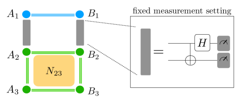
which is located at sites $A_{2}A_{3}B_{2}B_{3}$ , see Fig. 1. We then place a state of interest $\rho$ in at $A_{1}B_{1}$ , denoted by $\rho_{1}:=\rho^{(A_{1}B_{1})}$ . It holds that

\displaystyle\mathrm{tr}[\rho W]=16\leavevmode\nobreak\ \mathrm{tr}[\rho_{1}\otimes N_{23}(\frac{1}{2}\mathbbm{1}-|\phi^{+}\rangle_{A_{3}B_{3}}\langle\phi^{+}|)\otimes P^{(12)}].\leavevmode\nobreak\ \leavevmode\nobreak\

(2)

where $P^{(12)}=|\phi^{+}\rangle_{A_{1}A_{2}}\langle\phi^{+}|\otimes|\phi^{+}\rangle_{B_{1}B_{2}}\langle\phi^{+}|$ . One can find the expectation value by estimating a singlet fraction,

{}_{A_{3}B_{3}}\langle\phi^{+}|\mathrm{tr}_{12}[\rho_{1}\otimes N_{23}\leavevmode\nobreak\ P^{(12)}]|\phi^{+}\rangle_{A_{3}B_{3}}=\frac{1}{8}-\frac{1}{4}\mathrm{tr}[\rho W],\leavevmode\nobreak\ \leavevmode\nobreak\

(3)

where the left-hand-side can be obtained by preparing a network state followed by a fixed measurement. Once a Bell measurement reports an outcome $P^{(12)}$ , a singlet fraction is estimated by finding the probability of having outcome $|\phi^{+}\rangle$ on $A_{3}B_{3}$ . In fact, an entangled state $\rho$ is detected if the probability, i.e., the left-hand-side in Eq. (3), is greater than $1/8$ , since $\mathrm{tr}[\sigma_{\mathrm{sep}}W]\geq 0$ for all separable states $\sigma_{\mathrm{sep}}$ .

Experimental resources to obtain the left-hand side in Eq. (3) are summarized as follows. One prepares a four-partite network state $N_{23}$ . Note that for two-qubit cases, a network state in Eq. (1) is a variation of a Smolin state, a four-partite bound entangled state [38]. Note that a Smolin state has been realized with photonic qubits [39, 40, 41]. The detection scheme also needs a measurement in the basis $|\phi^{+}\rangle$ , which is equivalent to the capability of realizing a controlled-NOT gate, a Hadamard gate, and a fixed-measurement in the $z$ -direction; see also Fig. 1. All these are compatible with the resources to realize measurement-based quantum computing.

III.2 EWs via entanglement activation

To show a general construction of network states for arbitrary EWs for high-dimensional quantum systems, let us first recall the result in Ref. [42] that all EWs can be expressed in the following form,

\displaystyle W_{A_{2}B_{2}}=\mathrm{tr}_{A_{3}B_{3}}\big{[}N(\eta\mathbbm{I}-|\phi_{d}^{+}\rangle_{A_{3}B_{3}}\langle\phi_{d}^{+}|)\big{]},

(4)

for some multipartite network state $N:=N^{(A_{2}B_{2}A_{3}B_{3})}$ and a parameter $\eta\in[1/d,1)$ , where $|\phi_{d}^{+}\rangle=\sum_{j=0}^{d-1}|jj\rangle/\sqrt{d}$ . Note that the parameter $\eta$ satisfies the condition, $\eta\geq E_{d}[N]$ where $E_{d}$ is called a maximal singlet fraction,

	$\displaystyle E_{d}[N]$	$\displaystyle=$	$\displaystyle\sup_{\mathcal{F}}\leavevmode\nobreak\ \langle\phi_{d}^{+}\|\mathcal{F}[N]\|\phi_{d}^{+}\rangle\leavevmode\nobreak\ \mathrm{for\leavevmode\nobreak\ a\leavevmode\nobreak\ local\leavevmode\nobreak\ filtering\leavevmode\nobreak\ }\mathcal{F}$		(5)
			$\displaystyle\mathcal{F}[N]=\frac{K_{A}\otimes K_{B}NK_{A}^{\dagger}\otimes K_{B}^{\dagger}}{\mathrm{tr}[K_{A}^{\dagger}K_{A}\otimes K_{B}^{\dagger}K_{B}N]},$		(5)

where $K_{A}:\mathcal{H}_{A_{1}A_{2}}\rightarrow\mathbbm{C}^{d}$ and $K_{B}:\mathcal{H}_{B_{1}B_{2}}\rightarrow\mathbbm{C}^{d}$ . It is worth mentioning that EWs in Eq. (4) identify entangled states that activate a network state in the sense that

\displaystyle E_{d}[\sigma\otimes N]>\eta,\leavevmode\nobreak\ \mathrm{whereas}\leavevmode\nobreak\ {E_{d}[N]\leq\eta}.

(6)

In fact, all entangled states can be used to activate some other state: in Eq. (6) a state $\sigma$ is entangled if and only if it can activate some other entangled state $N$ .

III.3 General construction of network states

We now present a construction of a network state for a given EW, see Eq. (4). For convenience, let us consider an EW $W$ on $d\otimes d$ , and its decomposition may be found as follows,

\displaystyle W=\sum_{j}a_{j}W(j)^{T}\leavevmode\nobreak\ \mathrm{with}\leavevmode\nobreak\ W(j)\geq 0\leavevmode\nobreak\ \mathrm{and}\leavevmode\nobreak\ a_{j}\in\mathbbm{R},

so that one can choose normalized non-negative operators $\{\Pi(i)\geq 0\}$ and constants $\{c_{j}\}$ such that,

\displaystyle N_{23}=\sum_{j}c_{j}W(j)_{A_{2}B_{2}}\otimes\Pi(j)_{A_{3}B_{3}}

(7)

and

\displaystyle W_{2}^{T}=\leavevmode\nobreak\ k\,\mathrm{tr}_{3}[N_{23}(\eta\mathbbm{1}-|\phi_{d}^{+}\rangle_{A_{3}B_{3}}\langle\phi_{d}^{+}|)].

(8)

for some $\eta\geq 1/d$ and $k>0$ . One can find $\{a_{j}\}$ and $\{c_{j}\}$ are related as follow,

a_{j}=k\,c_{j}(\eta-\langle\phi_{d}^{+}|\Pi(j)|\phi_{d}^{+}\rangle).

For a state $\rho_{1}=\rho^{(A_{1}B_{1})}$ it holds that

\displaystyle\mathrm{tr}[\rho W]

\displaystyle\propto

\displaystyle\mathrm{tr}[\rho_{1}\otimes N_{23}\leavevmode\nobreak\ P^{(12)}\otimes(\eta\mathbbm{1}-|\phi_{d}^{+}\rangle_{A_{3}B_{3}}\langle\phi_{d}^{+}|)].\leavevmode\nobreak\ \leavevmode\nobreak\ \leavevmode\nobreak\

(9)

For an entangled state $\rho$ detected by $W$ , i.e., $\mathrm{tr}[\rho W]<0$ , Eq. (9) shows that

	$\displaystyle\eta$	$\displaystyle<$	${}_{A_{3}B_{3}}\langle\phi_{d}^{+}\|\Lambda^{(1\rightarrow 3)}[\rho_{1}]\|\phi_{d}^{+}\rangle_{A_{3}B_{3}}$		(10)
			$\displaystyle\mathrm{where}\leavevmode\nobreak\ \Lambda^{(1\rightarrow 3)}[\rho_{1}]=\frac{\mathrm{tr}_{12}[\rho_{1}\otimes N_{23}P^{(12)}]}{\mathrm{tr}[\rho_{1}\otimes N_{23}P^{(12)}]}.\leavevmode\nobreak\ \leavevmode\nobreak\$		(10)

The above may be rephrased by a teleportation protocol: once a measurement $P^{(12)}$ is successful, a state $\rho$ prepared at $A_{1}B_{1}$ is sent to $A_{3}B_{3}$ via a network state $N_{23}$ . Then, a singlet fraction is estimated and compared with $\eta$ , which is pre-determined by a network state to realize an EW. As mentioned, experimental resources for the realization contain preparing a network state and Bell measurements that require bi-interactions and a fixed local measurement setting; see also Fig. 1. In Appendix A, we reproduce a network state in Eq. (1) by applying the general construction above.

IV Examples

Let us then apply the general construction of network states and present network states for decomposable and non-decomposable EWs. We recall that identifying all EWs, equivalent to characterizing the set of separable states, is a challenging mathematical problem [35]. Its computational complexity also belongs to NP-Hard [43]. In what follows, we consider EWs known so far and show network states to construct them.

To this end, let $P_{st}$ denote a projection onto a Bell state, for $s,t=0,\ldots,d-1$ , in a dimension $d$ ,

\displaystyle P_{st}=|\phi_{st}\rangle\langle\phi_{st}|\leavevmode\nobreak\ \mathrm{where}\leavevmode\nobreak\ |\phi_{st}\rangle=\frac{1}{\sqrt{d}}\sum_{j=0}^{d-1}\omega^{tj}|j\rangle|j+s\rangle,\leavevmode\nobreak\ \leavevmode\nobreak\

(11)

where $\omega=e^{2\pi i/d}$ . Projectors onto symmetric and anti-symmetric subspaces are denoted by $S_{d}$ and $A_{d}$ , respectively,

\displaystyle S_{d}=\frac{\mathbbm{1+F}}{2}\leavevmode\nobreak\ \leavevmode\nobreak\ \mathrm{and}\leavevmode\nobreak\ \leavevmode\nobreak\ A_{d}=\frac{\mathbbm{1-F}}{2},

(12)

where $\mathbbm{F}=dP_{00}^{\Gamma}$ is a flip operator [32]. Note that $\mathrm{tr}[A_{d}]=d(d-1)/2$ and $\mathrm{tr}[S_{d}]=d(d+1)/2$ . Interestingly, high-dimensional Bell states and projections onto symmetric and anti-symmetric subspaces suffice to construct network states for known non-decomposable maps.

IV.1 Decomposable EWs: the partial transposition

Firstly, we consider a decomposable EW $W=Q^{\Gamma}$ for $Q\geq 0$ and $\mathrm{tr}[Q]=1$ , for which a network state can be constructed as follows. We write by $\lambda:=\max_{i}|\lambda_{i}|$ where $\{\lambda_{i}\}$ are eigenvalues of an EW $W$ and a network state is obtained as,

	$\displaystyle N_{23}$	$\displaystyle=$	$\displaystyle c_{1}\left(\frac{\lambda\mathbbm{1}-Q^{\Gamma}}{\lambda d^{2}-1}\right)^{(2)}\otimes P_{00}^{(3)}$		(13)
			$\displaystyle+c_{2}\left(\frac{\lambda\mathbbm{1}+Q^{\Gamma}}{\lambda d^{2}+1}\right)^{(2)}\otimes\left(\frac{\mathbbm{1}-P_{00}}{d^{2}-1}\right)^{(3)},$		(13)

where superscript $(j)$ stands for systems $A_{j}B_{j}$ and

\displaystyle c_{1}=\frac{d^{2}\lambda-1}{d^{3}\lambda+d-2}\leavevmode\nobreak\ \leavevmode\nobreak\ \mathrm{and}\leavevmode\nobreak\ \leavevmode\nobreak\ c_{2}=\frac{(d-1)(d^{2}\lambda+1)}{d^{3}\lambda+d-2}.

In the other way around, from a network state $N_{23}$ in Eq. (13) one can reproduce a decomposable EW, see Eq. (4)

\displaystyle\mathrm{tr}_{3}[N_{23}(\frac{1}{d}\mathbbm{1}-|\phi_{00}\rangle_{A_{3}B_{3}}\langle\phi_{00}|)]=\frac{2(d-1)}{d(d^{3}\lambda+d-2)}Q^{\Gamma}\propto Q^{\Gamma}.

Hence, the partial transpose criteria [44] can be generally realized by preparing a network state with a fixed measurement.

As an instance, a network state for the decomposable and optimal EW $W=P_{00}^{\Gamma}$ can be found as

\displaystyle\frac{1}{d+2}\left(\frac{A_{d}}{\mathrm{tr}A_{d}}\right)^{(2)}\otimes P_{00}^{(3)}+\frac{d+1}{d+2}\left(\frac{S_{d}}{\mathrm{tr}S_{d}}\right)^{(2)}\otimes\left(\frac{\mathbbm{1}-P_{00}}{d^{2}-1}\right)^{(3)}.

The network state above is known as a symmetric state being $UUVV^{*}$ -invariant, and has been used to activate entanglement distillation with an infinitesimal amount of bound entanglement [45].

IV.2 Non-decomposable EWs

Secondly, to construct network states for non-decomposable EWs, we introduce paired Bell-diagonal (PBD) states as follows,

\displaystyle N_{23}^{(\mathrm{PBD})}(\vec{\lambda})=\sum_{s=0}^{d-1}\lambda_{s}\leavevmode\nobreak\ \frac{1}{d}\sum_{t=0}^{d-1}P_{st}^{(2)}\otimes P_{st}^{(3)},

(14)

where $\vec{\lambda}=(\lambda_{0},\ldots,\lambda_{d-1})$ and $\sum_{s=0}^{d-1}\lambda_{s}=1$ .

IV.2.1 Bell-diagonal EWs

A network state in Eq. (14) can be used to estimate expectation values of Bell-diagonal EWs [23],

\displaystyle W[\vec{\lambda}]=\sum_{s=0}^{d-1}\lambda_{s}\Pi_{s}-P_{00},\leavevmode\nobreak\ \leavevmode\nobreak\ \mathrm{where}\leavevmode\nobreak\ \leavevmode\nobreak\ \Pi_{s}=\sum_{t=0}^{d-1}P_{st}.

(15)

Note that the Choi map and its generalizations are well-known instances. Then, PBD network states construct Bell-diagonal EWs as follows,

\displaystyle\frac{\lambda_{0}}{d}W_{2}^{T}[\vec{\lambda}]

\displaystyle=

\displaystyle\mathrm{tr}_{3}[N_{23}^{(\mathrm{PBD})}(\vec{\lambda})(\lambda_{0}\mathbbm{1}-|\phi_{00}\rangle_{A_{3}B_{3}}\langle\phi_{00}|)].

Hence, it is shown that all entangled states characterized by Bell-diagonal EWs can be detected by a fixed measurement and state preparation.

IV.2.2 Choi EWs

Instances of Bell-diagonal EWs for $d=3$ contain the Choi map [25] and its generalizations [26, 46], that detect PPT entangled states. As it is shown in Eq. (10), once a filtering operation with a PBD network state in Eq. (14) is successful, entangled states are concluded by finding a singlet fraction. For the case the Choi map, entangled states are detected if the singlet fraction is larger than $2/3$ . The proof is provided in Appendix B.

IV.2.3 Multipartite bound entangled states as a network state

We also observe that a PBD state for $d=2$ with $\vec{\lambda}=(1/2,1/2)$ corresponds to a Smolin state [38],

\displaystyle\rho_{S}=\frac{1}{4}\sum_{s,t=0,1}P_{st}^{(A_{2}B_{2})}\otimes P_{st}^{(A_{3}B_{3})}.

The state is invariant under permutations of $A_{2}A_{3}B_{2}B_{3}$ and remains PPT in any bipartite splitting: it is called a four-partite unlockable and undistillable entangled state. A Smolin state can be used to activate distillation of entanglement.

A Smolin state can be generalized to higher dimensions, with $\vec{\lambda}=(1/d,\ldots,1/d)$ ,

\displaystyle N_{23}(\vec{\lambda})=\frac{1}{d^{2}}\sum_{s=0}^{d-1}\sum_{t=0}^{d-1}P_{st}^{(A_{2}B_{2})}\otimes P_{st}^{(A_{3}B_{3})}.

However, a Smolin state in a higher dimension $d>2$ no longer remains PPT in the bipartite splitting $A_{2}A_{3}:B_{2}B_{3}$ . The network state then realizes an EW,

\displaystyle W=\frac{1}{d}\sum_{s=0}^{d-1}\Pi_{s}-P_{00}=\frac{1}{d}\mathbbm{1}-P_{00}

which is decomposable. It is also an EW that is derived from a reduction map [47]. Note that a Smolin state corresponds to a network state that realizes a reduction EW for $d=2$ .

IV.2.4 EWs from the Breuer-Hall map

The Breuer-Hall (BH) map shown in Refs. [27, 28] derives highly non-trivial non-decomposable EWs,

\displaystyle\Lambda_{\textrm{BH}}(\rho)=\frac{1}{d-2}(\mathrm{tr}(\rho)\mathbbm{1}-\rho-U\rho^{T}U^{\dagger})

(16)

where $U$ is an skew-symmetric unitary operator satisfying $UU^{\dagger}=\mathbbm{1}$ and $U^{T}=-U$ . Then the BH EW is obtained as follows,

\displaystyle W_{\mathrm{BH}}=\frac{1}{d-2}(\frac{1}{d}\mathbbm{1}-P_{00}-\frac{1}{d}\mathbbm{F}^{\prime}),

(17)

where $\mathbbm{F}^{\prime}\equiv(\mathbbm{1}\otimes U)\mathbbm{F}(\mathbbm{1}\otimes U^{\dagger})$ . Note that the BH EW is optimal.

A network state for the BH EW is obtained as follows,

$\displaystyle N_{23}^{(\textrm{BH})}$	$\displaystyle=$	$\displaystyle c_{0}\frac{1}{d^{2}}\sum_{s=0}^{d-1}\sum_{t=0}^{d-1}P_{st}^{(2)}\otimes P_{st}^{(3)}$	(18)
		$\displaystyle+c_{1}\left(\frac{\mathbbm{1}+\mathbbm{F}^{\prime}}{d^{2}+d}\right)^{(2)}\otimes P_{00}^{(3)}$
		$\displaystyle+c_{2}\left(\frac{\mathbbm{1}-\mathbbm{F}^{\prime}}{d^{2}-d}\right)^{(2)}\otimes\left(\frac{\mathbbm{1}-P_{00}}{d^{2}-1}\right)^{(3)},$

where

\displaystyle c_{0}=\frac{2d^{2}-2d}{3d^{2}-3d+2},\leavevmode\nobreak\ \mathrm{and}\leavevmode\nobreak\ c_{1}=\frac{d+1}{3d^{2}-3d+2},

and $c_{2}=1-c_{0}-c_{1}$ . One can find that, from Eq. (8)

\displaystyle W_{\mathrm{BH}}^{T}\leavevmode\nobreak\ \leavevmode\nobreak\ \propto\leavevmode\nobreak\ \leavevmode\nobreak\ \mathrm{tr}_{3}[N_{23}^{(\mathrm{BH})}\leavevmode\nobreak\ (\frac{1}{d}\mathbbm{1}-|\phi_{00}\rangle_{A_{3}B_{3}}\langle\phi_{00}|)].

(19)

Once a filtering operation in Eq. (10) is successful, entangled states are detected if a singlet fraction of a resulting state on $A_{3}B_{3}$ is larger than $1/d$ .

IV.3 EWs for multipartite systems

Thirdly, entanglement detection by state preparation can be extended to multipartite quantum states. We here, in particular, consider graph states, a class of states as a resource for measurement-based quantum computing [30]. Let us again present an instance for a three-qubit graph state, a Greenberger–Horne–Zeilinger (GHZ) state $|\psi\rangle=(|000\rangle+|111\rangle)/\sqrt{2}$ [48], see Fig. 2. An EW to detect a GHZ state may be given as,

\displaystyle W=\frac{1}{2}\mathbbm{1}-|\psi\rangle\langle\psi|.

(20)

A network state for an EW above can be constructed as,

\displaystyle N_{23}=\frac{1}{8}\sum_{a,b,c=0}^{1}\psi_{abc}^{(A_{2}B_{2}C_{2})}\otimes\psi_{abc}^{(A_{3}B_{3}C_{3})}.

(21)

where $\psi_{abc}=|\psi_{abc}\rangle\langle\psi_{abc}|$ ,

\displaystyle|\psi_{abc}\rangle=Z^{a}\otimes X^{b}\otimes X^{c}|\psi\rangle,\leavevmode\nobreak\ \leavevmode\nobreak\ a,b,c\in\{0,1\}

(22)

with Pauli matrices $X$ and $Z$ . It holds that

\displaystyle{}_{A_{3}B_{3}C_{3}}\langle\psi|\rho_{1}\otimes N_{23}\leavevmode\nobreak\ P^{(12)}|\psi\rangle_{A_{3}B_{3}C_{3}}=\frac{1}{16}-\frac{1}{8}\mathrm{tr}[\rho W],

which shows detection of a genuinely multipartite entangled state $\rho$ by finding that the left-hand-side is greater than $1/16$ . Further generalization for detecting entangled $n$ -qubit graph states is provided in Appendix C.

IV.4 To construct non-decomposable EWs

Finally, let us investigate two entangled states defined by an EW. One denotes an entangled state $\rho_{1}$ detected by an EW, and the other $N_{23}$ realizing an EW by its preparation; see also Eq. (4). The result in Ref. [42] shows that an EW detects a set of entangled states that can activate its network state. Since a pair of PPT states cannot activate each other, either the states $\rho_{1}$ or $N_{23}$ must be non-PPT. Hence, a network state $N_{23}$ to detect a PPT entangled state $\rho_{1}$ should be non-PPT. We thus conclude that multipartite non-PPT entangled states can construct non-decomposable EWs, which are then highly non-trivial.

Conclusion

In conclusion, we have established the framework of detecting entangled states in terms of state preparation and a fixed measurement. We have presented the construction of network states that allow one to estimate EWs. Network states for EWs known so far are explicitly provided, both decomposable and non-decomposable cases. Our results shed new light on detecting entangled states: a measurement setting for estimating EWs is replaced by a state preparation and then simplified to a fixed one.

Acknowledgement

This work is supported by National Research Foundation of Korea (NRF-2021R1A2C2006309, NRF-2022M1A3C2069728) and the Institute for Information & Communication Technology Promotion (IITP) (the ITRC Program/IITP-2023-2018-0-01402). AB and DC were supported by the Polish National Science Center project No. 2018/30/A/ST2/00837.

References

Terhal [2000] B. M. Terhal, Bell inequalities and the separability criterion, Physics Letters A 271, 319 (2000).
Lewenstein et al. [2000] M. Lewenstein, B. Kraus, J. I. Cirac, and P. Horodecki, Optimization of entanglement witnesses, Phys. Rev. A 62, 052310 (2000).
Horodecki et al. [1996] M. Horodecki, P. Horodecki, and R. Horodecki, Separability of mixed states: necessary and sufficient conditions, Physics Letters A 223, 1 (1996).
Gühne and Tóth [2009] O. Gühne and G. Tóth, Entanglement detection, Physics Reports 474, 1 (2009).
Horodecki et al. [2009] R. Horodecki, P. Horodecki, M. Horodecki, and K. Horodecki, Quantum entanglement, Rev. Mod. Phys. 81, 865 (2009).
Chruściński and Sarbicki [2014] D. Chruściński and G. Sarbicki, Entanglement witnesses: construction, analysis and classification, Journal of Physics A: Mathematical and Theoretical 47, 483001 (2014).
Friis et al. [2019] N. Friis, G. Vitagliano, M. Malik, and M. Huber, Entanglement certification from theory to experiment, Nature Reviews Physics 1, 72 (2019).
Branciard et al. [2013] C. Branciard, D. Rosset, Y.-C. Liang, and N. Gisin, Measurement-device-independent entanglement witnesses for all entangled quantum states, Phys. Rev. Lett. 110, 060405 (2013).
Bae et al. [2011] J. Bae, W.-Y. Hwang, and Y.-D. Han, No-signaling principle can determine optimal quantum state discrimination, Phys. Rev. Lett. 107, 170403 (2011).
Bowles et al. [2018] J. Bowles, I. Šupić, D. Cavalcanti, and A. Acín, Device-independent entanglement certification of all entangled states, Physical Review Letters 121, 180503 (2018).
Grover [1997] L. K. Grover, Quantum mechanics helps in searching for a needle in a haystack, Phys. Rev. Lett. 79, 325 (1997).
Quek and Shor [2017] Y. Quek and P. W. Shor, Quantum and superquantum enhancements to two-sender, two-receiver channels, Phys. Rev. A 95, 052329 (2017).
Yun et al. [2020] J. Yun, A. Rai, and J. Bae, Nonlocal network coding in interference channels, Phys. Rev. Lett. 125, 150502 (2020).
Acín et al. [2007] A. Acín, N. Brunner, N. Gisin, S. Massar, S. Pironio, and V. Scarani, Device-independent security of quantum cryptography against collective attacks, Phys. Rev. Lett. 98, 230501 (2007).
Pironio et al. [2009] S. Pironio, A. Acín, N. Brunner, N. Gisin, S. Massar, and V. Scarani, Device-independent quantum key distribution secure against collective attacks, New Journal of Physics 11, 045021 (2009).
Preskill [2018] J. Preskill, Quantum Computing in the NISQ era and beyond, Quantum 2, 79 (2018).
Krantz et al. [2019] P. Krantz, M. Kjaergaard, F. Yan, T. P. Orlando, S. Gustavsson, and W. D. Oliver, A quantum engineer’s guide to superconducting qubits, Applied Physics Reviews 6, 021318 (2019), https://doi.org/10.1063/1.5089550 .
Henriet et al. [2020] L. Henriet, L. Beguin, A. Signoles, T. Lahaye, A. Browaeys, G.-O. Reymond, and C. Jurczak, Quantum computing with neutral atoms, Quantum 4, 327 (2020).
Graham et al. [2022] T. M. Graham, Y. Song, J. Scott, C. Poole, L. Phuttitarn, K. Jooya, P. Eichler, X. Jiang, A. Marra, B. Grinkemeyer, M. Kwon, M. Ebert, J. Cherek, M. T. Lichtman, M. Gillette, J. Gilbert, D. Bowman, T. Ballance, C. Campbell, E. D. Dahl, O. Crawford, N. S. Blunt, B. Rogers, T. Noel, and M. Saffman, Multi-qubit entanglement and algorithms on a neutral-atom quantum computer, Nature 604, 457 (2022).
Doran and Society [1994] R. Doran and A. Society, C*-algebras: 1943-1993 : a Fifty Year Celebration : AMS Special Session Commemorating the First Fifty Years of C*-algebra Theory, January 13-14, 1993, San Antonio, Texas, Contemporary mathematics (American Mathematical Society, 1994).
Sparaciari and Paris [2013] C. Sparaciari and M. G. A. Paris, Canonical naimark extension for generalized measurements involving sets of pauli quantum observables chosen at random, Phys. Rev. A 87, 012106 (2013).
Yordanov and Barnes [2019] Y. S. Yordanov and C. H. W. Barnes, Implementation of a general single-qubit positive operator-valued measure on a circuit-based quantum computer, Phys. Rev. A 100, 062317 (2019).
Chruściński [2014] D. Chruściński, A class of symmetric bell diagonal entanglement witnesses—a geometric perspective, Journal of Physics A: Mathematical and Theoretical 47, 424033 (2014).
Bera et al. [2022a] A. Bera, F. A. Wudarski, G. Sarbicki, and D. Chruściński, Class of bell-diagonal entanglement witnesses in $\mathbbm{C}^{4}\otimes\mathbbm{C}^{4}$ : Optimization and the spanning property, Phys. Rev. A 105, 052401 (2022a).
Choi [1975] M.-D. Choi, Completely positive linear maps on complex matrices, Linear Algebra and its Applications 10, 285 (1975).
Ha and Kye [2011] K.-C. Ha and S.-H. Kye, One-parameter family of indecomposable optimal entanglement witnesses arising from generalized choi maps, Phys. Rev. A 84, 024302 (2011).
Breuer [2006] H.-P. Breuer, Optimal entanglement criterion for mixed quantum states, Phys. Rev. Lett. 97, 080501 (2006).
Hall [2006] W. Hall, A new criterion for indecomposability of positive maps, Journal of Physics A: Mathematical and General 39, 14119 (2006).
Hein et al. [2004] M. Hein, J. Eisert, and H. J. Briegel, Multiparty entanglement in graph states, Phys. Rev. A 69, 062311 (2004).
Raussendorf and Briegel [2001] R. Raussendorf and H. J. Briegel, A one-way quantum computer, Phys. Rev. Lett. 86, 5188 (2001).
Gühne et al. [2007] O. Gühne, C.-Y. Lu, W.-B. Gao, and J.-W. Pan, Toolbox for entanglement detection and fidelity estimation, Phys. Rev. A 76, 030305 (2007).
Dür et al. [2000a] W. Dür, J. I. Cirac, M. Lewenstein, and D. Bruß, Distillability and partial transposition in bipartite systems, Phys. Rev. A 61, 062313 (2000a).
Shor et al. [2001] P. W. Shor, J. A. Smolin, and B. M. Terhal, Nonadditivity of bipartite distillable entanglement follows from a conjecture on bound entangled werner states, Phys. Rev. Lett. 86, 2681 (2001).
Horodecki et al. [1999] P. Horodecki, M. Horodecki, and R. Horodecki, Bound entanglement can be activated, Physical review letters 82, 1056 (1999).
Størmer [1963] E. Størmer, Positive linear maps of operator algebras, Acta Mathematica 110, 233 (1963).
Bera et al. [2022b] A. Bera, G. Scala, G. Sarbicki, and D. Chruściński, Generalizing choi map in $m_{3}$ beyond circulant scenario, arXiv:2212.03807 (2022b).
Bera et al. [2022c] A. Bera, G. Sarbicki, and D. Chruściński, A class of optimal positive maps in $m_{n}$ , arXiv:2207.03821 (2022c).
Smolin [2001] J. A. Smolin, Four-party unlockable bound entangled state, Phys. Rev. A 63, 032306 (2001).
Amselem and Bourennane [2009] E. Amselem and M. Bourennane, Experimental four-qubit bound entanglement, Nature Physics 5, 748 (2009).
Lavoie et al. [2010] J. Lavoie, R. Kaltenbaek, M. Piani, and K. J. Resch, Experimental bound entanglement in a four-photon state, Phys. Rev. Lett. 105, 130501 (2010).
Kaneda et al. [2012] F. Kaneda, R. Shimizu, S. Ishizaka, Y. Mitsumori, H. Kosaka, and K. Edamatsu, Experimental activation of bound entanglement, Phys. Rev. Lett. 109, 040501 (2012).
Masanes [2006] L. Masanes, All bipartite entangled states are useful for information processing, Phys. Rev. Lett. 96, 150501 (2006).
Gurvits [2003] L. Gurvits, Classical deterministic complexity of edmonds’ problem and quantum entanglement, in Proceedings of the Thirty-Fifth Annual ACM Symposium on Theory of Computing, STOC ’03 (Association for Computing Machinery, New York, NY, USA, 2003) pp. 10–19.
Peres [1996] A. Peres, Separability criterion for density matrices, Phys. Rev. Lett. 77, 1413 (1996).
Vollbrecht and Wolf [2002] K. G. H. Vollbrecht and M. M. Wolf, Activating distillation with an infinitesimal amount of bound entanglement, Physical review letters 88, 247901 (2002).
Chruściński and Sarbicki [2013] D. Chruściński and G. Sarbicki, Optimal entanglement witnesses for two qutrits, Open Systems & Information Dynamics 20, 1350006 (2013), https://doi.org/10.1142/S1230161213500066 .
Horodecki and Horodecki [1999] M. Horodecki and P. Horodecki, Reduction criterion of separability and limits for a class of distillation protocols, Phys. Rev. A 59, 4206 (1999).
Dür et al. [2000b] W. Dür, G. Vidal, and J. I. Cirac, Three qubits can be entangled in two inequivalent ways, Phys. Rev. A 62, 062314 (a 2000b).
Jungnitsch et al. [2011] B. Jungnitsch, T. Moroder, and O. Gühne, Entanglement witnesses for graph states: General theory and examples, Phys. Rev. A 84, 032310 (2011).

Appendix A Entanglement detection by state preparation for two-qubit states

We here reproduce a network state for two-qubit EWs. Let $|\phi^{\pm}\rangle=(|00\rangle\pm|11\rangle)/\sqrt{2}$ and $|\psi^{\pm}\rangle=(|01\rangle\pm|10\rangle)/\sqrt{2}$ denote four Bell states. We show how to construct a network state for an EW

\displaystyle W=|\phi^{+}\rangle\langle\phi^{+}|^{\Gamma}=\frac{1}{2}\mathbbm{I}-|\psi^{-}\rangle\langle\psi^{-}|.

One may find a decomposition of the above EW in the following way

\displaystyle W=\frac{1}{2}(\mathbbm{I}-|\psi^{-}\rangle\langle\psi^{-}|)-\frac{1}{2}|\psi^{-}\rangle\langle\psi^{-}|,

where two non-negative operators are obtained as $|\psi^{-}\rangle\langle\psi^{-}|$ and $(\mathbbm{I}-|\psi^{-}\rangle\langle\psi^{-}|)/2$ . A network state may be written as

	$\displaystyle N_{23}$	$\displaystyle=$	$\displaystyle c_{1}\|\psi^{-}\rangle_{A_{2}B_{2}}\langle\psi^{-}\|\otimes\Pi_{A_{3}B_{3}}(1)+$
			$\displaystyle\frac{c_{2}}{3}(\mathbbm{I}-\|\psi^{-}\rangle_{A_{2}B_{2}}\langle\psi^{-}\|)\otimes\Pi_{A_{3}B_{3}}(2),$

for some positive constants $c_{1},\leavevmode\nobreak\ c_{2}=1-c_{1}>0$ and non-negative normalized operators $\Pi(1),\leavevmode\nobreak\ \Pi(2)\geq 0$ . To realize entanglement detection of a state of interest $\rho$ using an entanglement witness $W$ , one may seek $N_{23}$ that satisfy

\displaystyle\mathrm{tr}[\rho_{1}W_{1}]=16\leavevmode\nobreak\ \mathrm{tr}[\rho_{1}\otimes N_{23}(\eta\mathbbm{1}-|\phi^{+}\rangle_{A_{3}B_{3}}\langle\phi^{+}|)\otimes P^{(12)}],

with $\eta=1/2$ , since all two-qubit entangled states are distillable. The goal is now to find the parameters $c_{1},\leavevmode\nobreak\ c_{2},\leavevmode\nobreak\ \Pi(1)$ and $\Pi(2)$ that satisfy the relation in the above. The left-hand-side (lhs) is given by

\displaystyle\mathrm{lhs}=\frac{1}{2}-\langle\psi^{-}|\rho|\psi^{-}\rangle,

and the right-hand-side (rhs) by

	$\displaystyle\mathrm{rhs}$	$\displaystyle=$	$\displaystyle 2\mathrm{tr}[\rho_{2}^{T}N_{23}]-4\mathrm{tr}[\rho_{2}^{T}\otimes\|\psi^{-}\rangle\langle\psi^{-}\|N_{23}]$
		$\displaystyle=$	$\displaystyle c_{2}(\frac{2}{3}-\frac{4}{3}\langle\phi^{+}\|\Pi(2)\|\phi^{+}\rangle)+L\langle\psi^{-}\|\rho\|\psi^{-}\rangle,$

where

	$\displaystyle L$	$\displaystyle=$	$\displaystyle c_{1}(2-4\langle\phi^{+}\|\Pi(1)\|\phi^{+}\rangle)+$
			$\displaystyle c_{2}(-\frac{2}{3}+\frac{4}{3}\langle\phi^{+}\|\Pi(2)\|\phi^{+}\rangle).$

From the lhs and the rhs, one can find that

\displaystyle c_{2}(\frac{2}{3}-\frac{4}{3}\langle\phi^{+}|\Pi(1)|\phi^{+}\rangle)=\frac{1}{2}\leavevmode\nobreak\ \mathrm{and}\leavevmode\nobreak\ L=-1,

from which

			$\displaystyle c_{1}(2-4\langle\phi^{+}\|\Pi(1)\|\phi^{+}\rangle)=-\frac{1}{2}$
		$\displaystyle\iff$	$\displaystyle c_{1}=\frac{1}{8\langle\phi^{+}\|\Pi(1)\|\phi^{+}\rangle-4}>0.$

For convenience, we choose $\Pi(1)=|\phi^{+}\rangle\langle\phi^{+}|$ although it is not a unique choice. It follows that $c_{1}=1/4$ and $c_{2}=3/4$ . The consequence is that $\langle\phi^{+}|\Pi(2)|\phi^{+}\rangle=0$ . Thus, we have

\displaystyle\Pi(2)=\frac{1}{3}(\mathbbm{I}-|\phi^{+}\rangle\langle\phi^{+}|).

All these conclude a network state

	$\displaystyle N_{23}$	$\displaystyle=$	$\displaystyle\frac{1}{4}\|\psi^{-}\rangle_{A_{2}B_{2}}\langle\psi^{-}\|\otimes\|\phi^{+}\rangle_{A_{3}B_{3}}\langle\phi^{+}\|+$
			$\displaystyle\frac{1}{12}(\mathbbm{1}-\|\psi^{-}\rangle_{A_{2}B_{2}}\langle\psi^{-}\|)\otimes(\mathbbm{1}-\|\phi^{+}\rangle_{A_{3}B_{3}}\langle\phi^{+}\|).$

Note that a network state for an EW is not unique.

Appendix B Network states for high-dimensional EWs

B.1 The framework

Recall that for a given EW $W$ , we are looking for a network state $N_{23}=N^{(A_{2}B_{2}A_{3}B_{3})}$ , which are separable in $A_{2}B_{2}:A_{3}B_{3}$ , satisfying the following condition:

\displaystyle W_{2}^{T}\propto\mathrm{tr}_{3}[N_{23}(\eta\mathbbm{1}-P_{00})_{3}],

(23)

for some $\eta\in[\frac{1}{d},1)$ . It is easy to see that the following relation holds:

	$\displaystyle\mathrm{tr}[\rho_{1}W_{1}]$	$\displaystyle=$	$\displaystyle d^{2}\mathrm{tr}[\rho_{1}\otimes W_{2}^{T}P^{(12)}]$		(24)
		$\displaystyle\propto$	$\displaystyle\mathrm{tr}[\rho_{1}\otimes N_{23}\leavevmode\nobreak\ P^{(12)}\otimes(\eta\mathbbm{1}-P_{00})_{3}],$		(25)

where $P^{(12)}=P_{00}^{(A_{1}A_{2})}\otimes P_{00}^{(B_{1}B_{2})}$ denotes the Bell measurements on both sides. The scheme can be understood as follows. First, a filtering operation $\Lambda^{(1\to 3)}$ teleports the state $\rho_{1}$ to $A_{3}B_{3}$ , leaving a result state $\Lambda(\rho)$ :

\displaystyle\Lambda^{(1\to 3)}(\rho)=\frac{\mathrm{tr}_{12}[\rho_{1}\otimes N_{23}P^{(12)}]}{\mathrm{tr}[\rho_{1}\otimes N_{23}P^{(12)}]}.

(26)

Then the singlet fraction, or the overlap with the Bell state $P_{00}$ , of the resulting state $\Lambda(\rho)$ is checked whether it is higher than $\eta$ or not.

The singlet fraction can also be estimated with a fixed measurement on individual quantum systems. The main idea is to place unitary interactions before a measurement. A $d$ -dimensional Hadamard gate and a $d$ -dimensional CNOT gate may be obtained as,

	$\displaystyle H$	$\displaystyle=\sum_{j,k=0}^{d-1}e^{2\pi ijk/d}\|j\rangle\langle k\|,\leavevmode\nobreak\ \mathrm{and}$
	$\displaystyle U_{CNOT}$	$\displaystyle=\sum_{j=0}^{d-1}\|j\rangle\langle j\|\otimes\sum_{k=0}^{d-1}\|k+j\rangle\langle k\|.$

Note that a maximally entangled state can be generated, $|\phi_{00}\rangle=U_{CNOT}(H\otimes\mathbbm{1})|00\rangle$ . Then, instead of a joint measurement, one can first apply $(H^{\dagger}\otimes\mathbbm{1})U_{CNOT}^{\dagger}$ to a resulting state $\Lambda^{(1\to 3)}(\rho)$ and then perform a measurement in the computational basis. The probability of having outcomes $00$ gives the singlet fraction $\langle\phi_{00}|\Lambda(\rho)|\phi_{00}\rangle$ . It holds that $\langle\phi_{00}|\Lambda(\rho)|\phi_{00}\rangle>\eta$ if and only if $\mathrm{tr}[\rho W]<0$ , which certifies that a state $\rho$ given in the beginning is entangled.

B.2 Decomposable EW

Consider a decomposable EW $W=Q^{\Gamma}$ for $Q\geq 0$ and $\mathrm{tr}[Q]=1$ . Let $\lambda:=\max_{i}|\lambda_{i}|$ where $\{\lambda_{i}\}$ are eigenvalues of $W$ . Then, a network state for the EW is obtained as

	$\displaystyle N_{23}^{\text{(dec)}}$	$\displaystyle=$	$\displaystyle c_{1}\left(\frac{\lambda\mathbbm{1}-Q^{\Gamma}}{\lambda d^{2}-1}\right)^{(2)}\otimes P_{00}^{(3)}$		(27)
			$\displaystyle+c_{2}\left(\frac{\lambda\mathbbm{1}+Q^{\Gamma}}{\lambda d^{2}+1}\right)^{(2)}\otimes\left(\frac{\mathbbm{1}-P_{00}}{d^{2}-1}\right)^{(3)},\leavevmode\nobreak\ \leavevmode\nobreak\$		(27)

with the threshold value $\eta=\frac{1}{d}$ ,

\displaystyle c_{1}=\frac{d^{2}\lambda-1}{d^{3}\lambda+d-2}\leavevmode\nobreak\ \leavevmode\nobreak\ \mathrm{and}\leavevmode\nobreak\ \leavevmode\nobreak\ c_{2}=\frac{(d-1)(d^{2}\lambda+1)}{d^{3}\lambda+d-2}.

The superscript $(j)$ stands for the composite space $A_{j}B_{j}$ for $j\in\{1,2,3\}$ . From the equation

\displaystyle\mathrm{tr}_{3}[N_{23}(\frac{1}{d}\mathbbm{1}-P_{00})_{3}]=\frac{2(d-1)}{d(d^{3}\lambda+d-2)}Q^{\Gamma},

it holds that

	$\displaystyle\mathrm{tr}[\rho W]=k\leavevmode\nobreak\ \mathrm{tr}[\rho_{1}\otimes N_{23}\leavevmode\nobreak\ P^{(12)}\otimes(\frac{1}{d}\mathbbm{1}-P_{00})_{3}],$
	$\displaystyle\langle\phi_{00}\|\Lambda(\rho)\|\phi_{00}\rangle>\frac{1}{d}\iff\mathrm{tr}[\rho W]<0,$		(28)

where $k=\frac{d(d^{3}\lambda+d-2)}{2(d-1)}$ .

Hence, the partial transpose criteria can be realized by preparing a network state in Eq. (27). In particular, a network state for the decomposable EW

\displaystyle W=P_{00}^{\Gamma}=\frac{\mathbbm{F}}{d},

(29)

which is proportional to the flip operator $\mathbbm{F}$ that detects entangled Werner states, can be found as

	$\displaystyle N_{23}^{\text{(flip)}}$	$\displaystyle=$	$\displaystyle\frac{1}{d+2}\left(\frac{\mathbbm{1}-\mathbbm{F}}{d^{2}-d}\right)^{(2)}\otimes P_{00}^{(3)}$		(30)
			$\displaystyle+\frac{d+1}{d+2}\left(\frac{\mathbbm{1}+\mathbbm{F}}{d^{2}+d}\right)^{(2)}\otimes\left(\frac{\mathbbm{1}-P_{00}}{d^{2}-1}\right)^{(3)}.\leavevmode\nobreak\ \leavevmode\nobreak\$		(30)

Note that this network state is invariant under $U_{A_{2}}\otimes U_{B_{2}}\otimes V_{A_{3}}\otimes V^{*}_{B_{3}}$ for any unitary operation $U,V$ . This network state is positive under the partial transpose $A_{2}A_{3}:B_{2}B_{3}$ , so it is undistillable. This state (30) has been used in the activation of non-PPT entangled states and proved to be PPT in [45].

B.3 Bell-diagonal EW

The next examples are Bell-diagonal witnesses $W(\vec{\lambda})$ , which are decomposable or non-decomposable depending on the parameter $\vec{\lambda}=(\lambda_{0},\ldots,\lambda_{d-1})$ :

\displaystyle W(\vec{\lambda})=\sum_{s=0}^{d-1}\lambda_{s}\Pi_{s}-P_{00},

(31)

where $\lambda_{s}\geq 0\leavevmode\nobreak\ \forall s$ and $\sum_{s=0}^{d-1}\lambda_{s}=1$ . Note also that $W[\vec{\lambda}]$ in Eq. (31) is an EW if a vector $\vec{\lambda}$ satisfies the cyclic inequalities in the following,

\displaystyle\sum_{j=0}^{d-1}\frac{t_{j}^{2}}{\sum_{s=0}^{d-1}\lambda_{s}t_{j+s}^{2}}\leq d,

for all $t_{0},\ldots,t_{d}\geq 0$ . The value $\lambda_{0}$ is critical in implementing this witness with state preparation, as shown below. To construct a network state for a Bell-diagonal EW, we use paired Bell-diagonal (PBD) states:

\displaystyle N_{23}^{\textrm{(PBD)}}(\vec{\lambda})=\sum_{s=0}^{d-1}\lambda_{s}\frac{1}{d}\sum_{t=0}^{d-1}P_{st}^{(2)}\otimes P_{st}^{(3)},

(32)

with the threshold value $\eta=\lambda_{0}$ . Then the following holds:

	$\displaystyle\mathrm{tr}[\rho W(\vec{\lambda})]=k\leavevmode\nobreak\ \mathrm{tr}[\rho_{1}\otimes N_{23}^{\textrm{(PBD)}}(\vec{\lambda})\leavevmode\nobreak\ P^{(12)}\otimes(\lambda_{0}\mathbbm{1}-P_{00})_{3}],$
	$\displaystyle\langle\phi_{00}\|\Lambda(\rho)\|\phi_{00}\rangle>\lambda_{0}\iff\mathrm{tr}[\rho W(\vec{\lambda})]<0.$

where $k=d^{3}/\lambda_{0}$ . It is possible to achieve $\langle\phi_{00}|\Lambda(\sigma)|\phi_{00}\rangle=\lambda_{0}$ with a separable state $\sigma$ :

	$\displaystyle\Lambda^{(1\to 3)}(\sigma)$	$\displaystyle=$	$\displaystyle\frac{\mathrm{tr}_{12}[\sigma_{1}\otimes N_{23}P^{(12)}]}{\mathrm{tr}[\sigma_{1}\otimes N_{23}P^{(12)}]},$
	$\displaystyle\textrm{where }\sigma$	$\displaystyle=$	$\displaystyle\frac{1}{d}P_{00}+\frac{1}{d}\sum_{s=1}^{d-1}\frac{\Pi_{s}}{d}.$

In particular, EWs from a reduction map and the Choi map can be written in the form of Bell-diagonal witness and can be implemented by preparing the corresponding PBD state. A decomposable EW from the reduction map corresponds to a Bell-diagonal EW with $\vec{\lambda}=(\frac{1}{d},\ldots,\frac{1}{d})$ :

	$\displaystyle W_{\textrm{red}}$	$\displaystyle=$	$\displaystyle\sum_{s=0}^{d-1}\frac{1}{d}\Pi_{s}-P_{00}=\frac{1}{d}\mathbbm{1}-P_{00},$		(33)
	$\displaystyle N_{23}^{\textrm{(red)}}$	$\displaystyle=$	$\displaystyle\frac{1}{d^{2}}\sum_{s=0}^{d-1}\sum_{t=0}^{d-1}P_{st}^{(2)}\otimes P_{st}^{(3)},$		(34)

with the threshold value $\eta=\frac{1}{d}$ .

The PBD state $N_{23}^{\textrm{(red)}}$ can be seen as a direct generalization of Smolin state [38] into $d$ -dimension. In $d=2$ , Smolin state is PPT in $A_{2}A_{3}:B_{2}B_{3}$ . However, the state $N_{23}^{\textrm{(red)}}$ is not PPT in higher dimensions $d\geq 3$ in general. Smolin state in two-dimension is undistillable, but the distillability of $N_{23}^{\textrm{(red)}}$ in higher dimensions is unknown.

Although it can be generalized into higher dimensions [26, 46], the nondecomposable witness from Choi map [25] is defined in $d=3$ and corresponds to a Bell-diagonal witness with $\vec{\lambda}=(\frac{2}{3},\frac{1}{3},0)$ :

	$\displaystyle W_{\textrm{Choi}}$	$\displaystyle=$	$\displaystyle\frac{2}{3}\Pi_{0}+\frac{1}{3}\Pi_{1}-P_{00},$		(35)
	$\displaystyle N_{23}^{\textrm{(Choi)}}$	$\displaystyle=$	$\displaystyle\frac{2}{9}\sum_{t=0}^{2}P_{0,t}^{(2)}\otimes P_{0,t}^{(3)}+\frac{1}{9}\sum_{t=0}^{2}P_{1,t}^{(2)}\otimes P_{1,t}^{(3)},\leavevmode\nobreak\ \leavevmode\nobreak\ \leavevmode\nobreak\ \leavevmode\nobreak\ \leavevmode\nobreak\ \leavevmode\nobreak\$		(36)

with the threshold value $\eta=\frac{2}{3}$ .

B.4 Breuer-Hall EW

The Breuer-Hall map [27, 28] finds an EW,

\displaystyle W_{\textrm{BH}}=\frac{1}{d}(\mathbbm{1}-\mathbbm{F}^{\prime})-P_{00},

(37)

where $\mathbbm{F}^{\prime}=(\mathbbm{1}\otimes U)\mathbbm{F}(\mathbbm{1}\otimes U^{\dagger})$ for any skew-symmetric unitary operator $U$ such that $UU^{\dagger}=\mathbbm{1}$ and $U^{T}=-U$ . In even dimensions $d=2n$ , one can set $U$ as

\displaystyle U=\operatorname*{\bigoplus}_{i=1}^{n}\begin{bmatrix}0&1\\ -1&0\end{bmatrix},

then it acts as $U|i\rangle=(-1)^{j}|j\rangle$ where $j=i+1$ for even $i$ and $j=i-1$ for odd $i$ .

One can think of $W_{\textrm{BH}}$ as a combination of reduction EW (33) and the flip operator from reduction map with additional $U$ . A network state for the BH EW is as follows,

$\displaystyle N_{23}^{(\textrm{BH})}$	$\displaystyle=$	$\displaystyle c_{0}\frac{1}{d^{2}}\sum_{s=0}^{d-1}\sum_{t=0}^{d-1}P_{st}^{(2)}\otimes P_{st}^{(3)}$	(38)
		$\displaystyle+c_{1}\left(\frac{\mathbbm{1}+\mathbbm{F}^{\prime}}{d^{2}+d}\right)^{(2)}\otimes P_{00}^{(3)}$
		$\displaystyle+c_{2}\left(\frac{\mathbbm{1}-\mathbbm{F}^{\prime}}{d^{2}-d}\right)^{(2)}\otimes\left(\frac{\mathbbm{1}-P_{00}}{d^{2}-1}\right)^{(3)},\leavevmode\nobreak\ \leavevmode\nobreak\ \leavevmode\nobreak\ \leavevmode\nobreak\$

with the threshold value $\eta=\frac{1}{d}$ , where $c_{0}=\frac{2d^{2}-2d}{3d^{2}-3d+2}$ , $c_{1}=\frac{d+1}{3d^{2}-3d+2}$ , and $c_{2}=\frac{d^{2}-2d+1}{3d^{2}-3d+2}$ . One can show that

\displaystyle\mathrm{tr}_{3}[N_{23}^{(\mathrm{BH})}\leavevmode\nobreak\ (\eta\mathbbm{1}-P_{00})_{3}]=\frac{c_{0}}{d^{2}}W_{\mathrm{BH}}^{T},

(39)

which leads to

	$\displaystyle\mathrm{tr}[\rho W_{\textrm{BH}}]=k\leavevmode\nobreak\ \mathrm{tr}[\rho_{1}\otimes N_{23}^{\textrm{(BH)}}\leavevmode\nobreak\ P^{(12)}\otimes(\eta\mathbbm{1}-P_{00})_{3}],$
	$\displaystyle\langle\phi_{00}\|\Lambda(\rho)\|\phi_{00}\rangle>\frac{1}{d}\iff\mathrm{tr}[\rho W_{\textrm{BH}}]<0,$

where $k=d^{4}/c_{0}$ .

Appendix C Entanglement witnesses for graph states

A graph $G=(V,E)$ is defined by a set of vertices $V$ and a set of edges $E$ :

	$\displaystyle V$	$\displaystyle=$	$\displaystyle\{1,\ldots,n\},\leavevmode\nobreak\ \text{where $n$ is the number of vertices,}$
	$\displaystyle E$	$\displaystyle=$	$\displaystyle\{(i,j)\|i,j\in V,i<j,\text{Vertex $i$ and $j$ are connected.}\}$

Also define the neighborhood of vertex $i$ : $E_{i}=\{j\in V|(i,j)\in E\text{ or }(j,i)\in E\}$ , which is a set of vertices connected to vertex $i$ .

The generators $g_{i}$ and the projectors $\gamma_{i}$ of a graph state determined by the graph $G$ are given by

	$\displaystyle g_{i}$	$\displaystyle=$	$\displaystyle X_{i}\prod_{j\in E_{i}}Z_{j},$
	$\displaystyle\gamma_{i}^{(x_{i})}$	$\displaystyle=$	$\displaystyle\frac{\mathbbm{1}+(-1)^{x_{i}}g_{i}}{2}.$		(40)

Note that the eigenvalue of $g_{i}$ is either 1 or -1, and the eigenvalue of $\gamma_{i}$ is either 1 or 0. Now we define an orthonormal graph state basis consisting of $2^{n}$ states:

\displaystyle|\vec{x}\rangle\langle\vec{x}|_{G}=\prod_{i=1}^{n}\gamma_{i}^{(x_{i})},\leavevmode\nobreak\ \leavevmode\nobreak\ \text{where }\vec{x}=(x_{1},\ldots,x_{n})\in\{0,1\}^{n}.

The states $|\vec{x}\rangle_{G}$ are the eigenstates of the generators and projectors:

	$\displaystyle g_{i}\|\vec{x}\rangle_{G}$	$\displaystyle=$	$\displaystyle(-1)^{x_{i}}\|\vec{x}\rangle_{G},$		(41)
	$\displaystyle\gamma_{i}^{(k)}\|\vec{x}\rangle_{G}$	$\displaystyle=$	$\displaystyle\begin{cases}\|\vec{x}\rangle_{G}&\mbox{if}\;x_{i}=k,\\ 0&\mbox{if}\;x_{i}\neq k.\end{cases}$		(42)

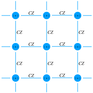
A graph state, denoted by $|\vec{0}\rangle\langle\vec{0}|_{G}$ , corresponds to an eigenstate with eigenvalue $+1$ for all generators $g_{i}$ ( $i\in\{1,\ldots,n\}$ ). A state can be obtained by preparing $|+\rangle=(|0\rangle+|1\rangle)/\sqrt{2}$ placed at vertices in $V$ , and applying the controlled-Z ( $CZ$ ) gate to all edges in $E$ , see Fig. 4.

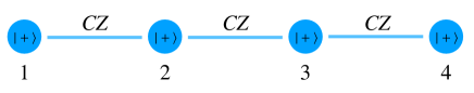
For instance, the four-qubit linear cluster state can be defined by a graph $G_{Cl4}=(V_{4},E_{Cl4})$ , where $V_{4}=\{1,2,3,4\}$ and $E_{Cl4}=\{(1,2),(2,3),(3,4)\}$ , see Fig. 5. The generators define $16$ graph states $|0000\rangle\langle 0000|_{G},\ldots,$ and $|1111\rangle\langle 1111|_{G}$ . The graph state $|0000\rangle\langle 0000|_{G}$ is detected by an EW in the following,

\displaystyle W_{Cl4}=\frac{1}{2}\sum_{\vec{x}\in S}|\vec{x}\rangle\langle\vec{x}|_{G}-|0000\rangle\!\langle 0000|_{G},

(43)

where $S=\{$ 0000, 0001, 0010, 0011, 0100, 0101, 0110, 0111, 1000, 1010, 1100, 1110 $\}$ . Then the network state for this graph state can be constructed by

\displaystyle N_{23}^{(Cl4)}=\sum_{\vec{x}\in S}\frac{1}{12}|\vec{x}\rangle\!\langle\vec{x}|_{G}^{(2)}\otimes|\vec{x}\rangle\!\langle\vec{x}|_{G}^{(3)}.

(44)

It holds that

	$\displaystyle\mathrm{tr}[\rho_{1}\otimes N_{23}^{(Cl4)}P^{(12)}\otimes(\frac{1}{2}\mathbbm{1}-\|0000\rangle\!\langle 0000\|_{G})]$
	$\displaystyle\propto\mathrm{tr}[\rho W_{Cl4}],$		(45)

where

	$\displaystyle P^{(12)}$	$\displaystyle=$	$\displaystyle\|\phi^{+}\rangle_{A_{1}A_{2}}\langle\phi^{+}\|\otimes\|\phi^{+}\rangle_{B_{1}B_{2}}\langle\phi^{+}\|$
			$\displaystyle\otimes\|\phi^{+}\rangle_{C_{1}C_{2}}\langle\phi^{+}\|\otimes\|\phi^{+}\rangle_{D_{1}D_{2}}\langle\phi^{+}\|.$

Then a four-qubit entangled state $\rho$ is detected by $W_{Cl4}$ when

\displaystyle{}_{G}\langle 0000|\Lambda[\rho]|0000\rangle_{G}>\frac{1}{2},

(46)

where the map $\Lambda^{(1\to 3)}$ is defined as,

\displaystyle\Lambda^{(1\rightarrow 3)}[\rho]=\frac{\mathrm{tr}_{12}[\rho_{1}\otimes N_{23}P^{(12)}]}{\mathrm{tr}[\rho_{1}\otimes N_{23}P^{(12)}]}.

A typical decomposable EW can be written in the following form [49]:

\displaystyle W_{G}=\frac{1}{2}\sum_{\vec{x}\in S}|\vec{x}\rangle\!\langle\vec{x}|_{G}-|\vec{0}\rangle\!\langle\vec{0}|_{G},

(47)

where the set $S\subseteq\{0,1\}^{n}$ depends on $W_{G}$ . Then the network states $N_{23}^{G}$ for this entanglement witnesses are given by

\displaystyle N_{23}^{(G)}=\sum_{\vec{x}\in S}\frac{1}{|S|}|\vec{x}\rangle\!\langle\vec{x}|_{G}^{(2)}\otimes|\vec{x}\rangle\!\langle\vec{x}|_{G}^{(3)}.

(48)

An $n$ -qubit entangled state $\rho$ is detected by $W_{G}$ when

\displaystyle{}_{G}\langle\vec{0}|\Lambda[\rho]|\vec{0}\rangle_{G}

\displaystyle>

\displaystyle\frac{1}{2},

(49)

for

	$\displaystyle\Lambda^{(1\rightarrow 3)}[\rho]$	$\displaystyle=$	$\displaystyle\frac{\mathrm{tr}_{12}[\rho_{1}\otimes N_{23}P^{(12)}]}{\mathrm{tr}[\rho_{1}\otimes N_{23}P^{(12)}]},$
	$\displaystyle P^{(12)}$	$\displaystyle=$	$\displaystyle\operatorname*{\bigotimes}_{v\in V}\|\phi^{+}\rangle_{v_{1}v_{2}}\langle\phi^{+}\|,$

where $V$ denotes the set of vertices of the graph $G$ .

The overlap ${}_{G}\langle\vec{0}|\Lambda[\rho]|\vec{0}\rangle_{G}$ can be estimated with a fixed measurement on individual qubits. Note that a graph state is generated as follows, $|\vec{0}\rangle_{G}$ is obtained as $|\vec{0}\rangle_{G}=(\operatorname*{\bigotimes}_{e\in E}U_{CZ})(\operatorname*{\bigotimes}_{v\in V}H)|0\rangle^{\otimes n}$ . Then, the estimation of a singlet fraction can be achieved by applying an interaction $(\operatorname*{\bigotimes}_{v\in V}H)(\operatorname*{\bigotimes}_{e\in E}U_{CZ})$ to a resulting state $\Lambda^{(1\to 3)}[\rho]$ and then performing a measurement in the computational basis. The probability of obtaining an outcome $00$ gives the overlap ${}_{G}\langle\vec{0}|\Lambda[\rho]|\vec{0}\rangle_{G}$ . It holds that ${}_{G}\langle\vec{0}|\Lambda[\rho]|\vec{0}\rangle_{G}>\frac{1}{2}$ if and only if $\mathrm{tr}[\rho W]<0$ , which certifies that $\rho$ is entangled.